BEC-BCS crossover and universal relations in unitary Fermi gases

Abstract

The contact parameter in unitary Fermi Gases governs the short-range correlations, and high-momentum properties of the system. We perform accurate quantum Monte Carlo calculations with highly optimized trial functions to precisely determine this parameter at T=0, demonstrate its universal application to a variety of observables, and determine the regions of momentum and energy over which the leading short-range behavior is dominant. We derive Tan’s expressions for the contact parameter using just the short-range behavior of the ground-state many-body wave function, and use this behavior to calculate the two-body distribution function, one-body density matrix, and the momentum distribution of unitary Fermi gases; providing a precise value of the contact parameter that can be compared to experiments.

The experimental realization and concurrent theoretical calculations of two-component unitary Fermi gases with short-range interactions offer a unique opportunity to test our understanding of strongly-interacting Fermi systems, and to study their structure and dynamics. The low-energy properties of the system are governed by the Bertsch parameter $\xi$, the pairing gap $\delta$, and have been studied extensively in the literature Giorgini:2008 ; *Carlson:2005; *Carlson:2008; Schirotzek:2008 ; *Lee:2008. The short-range correlations of the system are, in contrast, governed by the many-body wave function at small interparticle separations, as encoded in the contact parameter $C$.

Tan, in a series of papers Tan_a:2008 ; Tan_b:2008 ; Tan_c:2008 , showed that in Fermi gases, if the effective range of the interaction is much smaller than any other length scale of the system, several universal relations occur, and related them to a parameter $C$ he called the contact parameter (see also Ref. Braaten:2010 for a review). In particular, the large momentum tail of the momentum distribution $N(k)$, behaves like $C/k^{4}$. This same parameter gives the small distance behavior of the two-body distribution function, and the derivative of the ground-state energy with respect to the inverse of the scattering length. Having multiple phenomena that depend on a single universal parameter means that the parameter can be calculated and measured in multiple ways, and in the range of validity of the experiments and the calculations, they must give the same results for the parameters. We employ highly-optimized trial wave functions and accurate quantum Monte Carlo to calculate several of these observables, and to extract the contact parameter. We thus produce more accurate results for the leading behavior and simultaneously determine the regimes where it is dominant.

Recently, several experimental measurements have measured $C$ using a variety of techniques Navon:2010 ; *Kuhnle:2010; *Stewart:2010; *Hu:2010. Values for the contact parameter have been calculated from previous results from quantum Monte Carlo Lobo:2006 ; *Combescot:2006; *Drut; *Su:2010; *Abe:2009 and other methods  Palestini:2010 ; *Chen:2007; *Lee:2008b. However, previous quantum Monte Carlo calculations give values of the contact at unitarity that disagree with each other at the 5 to 10 percent level. Here we show that if the calculations are carefully optimized and extrapolated to zero range, our quantum Monte Carlo results agree with each other within statistical errors, less than 0.5 percent, giving clear numerical evidence of Tan’s predicted universal contact parameter and its behavior around unitarity. Our results provide a benchmark prediction for low temperature experiments.

We perform variational and fixed-node diffusion Monte Carlo (VMC and DMC) calculations of a system of a homogeneous system of fermions interacting with a short range potential. Fixed-node diffusion Monte Carlo results produce upper bounds to the ground-state energy of the system depending only upon the nodes (zeroes) of the trial wave function. We carefully optimize the trial wave functions, and obtain the best upper bounds to date for the ground state energy. Observables other than the ground-state energy are calculated by extrapolating the variational and mixed estimates: $O_{V}=\langle\Psi_{T}|O|\Psi_{T}\rangle$ and $O_{m}=\langle\Psi_{0}|O|\Psi_{T}\rangle$ , $\langle O\rangle\approx 2O_{m}-O_{V}.$ After suitable optimizations the extrapolations are very small. We calculate the contact parameter in several different ways and show they all give results consistent with each other and with recent experiments.

Tan and later others Tan_a:2008 ; *Tan_b:2008; *Tan_c:2008; Braaten:2008 ; *Combescot:2009; *Werner:2009 derived expressions for his contact parameter using a variety of methods. These results can be understood as coming from the behavior of the many-body wave function when two unlike spin particles are separated by a distance $r$ small compared to the average particle separation, $r_{0}$, but outside the range of the potential, $R$,

$$f(r)=\frac{A(1-a^{-1}r)}{r}\,,$$ (1)

($a$ is the two-body scattering length) which is Eq. 1 in Tan_a:2008 and $A^{2}$ will be seen to be proportional to Tan’s contact parameter $C$. The unlike spin two-body distribution function will be given by $f^{2}(r)$ in this same range

$$g_{\uparrow\downarrow}(r)=A^{2}(r^{-2}-2a^{-1}r^{-1}+\dots)\,,$$ (2)

where $g_{\uparrow\downarrow}(r\rightarrow\infty)=\frac{1}{2}$ for an unpolarized system. The momentum distribution summed over both spins will also be dominated by this short range part of the wave function, so for $k$ much greater than the Fermi momentum $k_{F}$ but much less than the inverse potential range, we have

$$\begin{split}&N(k)=n\int d^{3}r\,dR\,\Psi(\mathbb{r}_{1}+\mathbb{r},\dots,\mathbb{r}_{N})\Psi(\mathbb{r}_{1},\dots,\mathbb{r}_{N})e^{-i\mathbb{k}\cdot\mathbb{r}}\\ &=n^{2}\int d^{3}r\,d^{3}r^{\prime}\,\frac{f(|\mathbb{r}+\mathbb{r}^{\prime}|)}{f(r^{\prime})}g_{\uparrow\downarrow}(r^{\prime})e^{-i\mathbb{k}\cdot\mathbb{r}}\\ &=n^{2}\int d^{3}r\,d^{3}r^{\prime}\,f(|\mathbb{r}+\mathbb{r}^{\prime}|)f(r^{\prime})e^{-i\mathbb{k}\cdot\mathbb{r}}=\frac{16\pi^{2}n^{2}A^{2}}{k^{4}}\,,\end{split}$$

where $dR$ indicates integration over $r_{1},\dots,r_{N}$, and $n$ is the number density. Fourier transforming the momentum distribution and the two-body distribution functions gives the behavior for the one-body density matrix (normalized to 1 at the origin) and the opposite spin static structure factor (which goes to $\tfrac{1}{2}$ for $k\rightarrow\infty$) of

$$\rho^{(1)}(r) = 1-2\pi nA^{2}r+\dots$$

$$S_{\uparrow\downarrow}(k)-\frac{1}{2} = \frac{2\pi^{2}nA^{2}}{k}\left[1-\frac{1}{4\pi ak}\right]+\dots\,.$$ (3)

Tan also related the contact parameter to the derivative of the energy with respect to the inverse scattering length. Changing the scattering length by changing the potential with the mass fixed and using the Hellman-Feynman theorem Hellmann:1937 ; *Feynman:1939

$$\frac{dE\quad}{da^{-1}}=\frac{n}{2}\int d^{3}r\,g_{\uparrow\downarrow}(r)\frac{dv(r)}{da^{-1}}$$ (4)

where $E$ is the energy per particle. Since $v(r)$ is nonzero only inside $R$, where the two-body potential is very strong, $g(r)$ can be replaced with $f^{2}(r)$ where $\frac{\hbar^{2}}{m}\nabla^{2}f(r)=v(r)f(r)$ and the integration taken over a sphere of radius $R$. Therefore

$$\begin{split}&\frac{dE\quad}{da^{-1}}=\frac{n}{2}\left[\frac{d}{da^{-1}}\int d^{3}r\,f^{2}(r)v(r)-2\int d^{3}r\,f(r)v(r)\frac{df(r)}{da^{-1}}\right]\\ &=\frac{\hbar^{2}n}{2m}\left[\frac{d}{da^{-1}}\int d^{3}r\,f(r)\nabla^{2}f(r)-2\int d^{3}r\,[\nabla^{2}f(r)]\frac{df(r)}{da^{-1}}\right]\\ &=\frac{2\pi\hbar^{2}n}{m}R^{2}\left.\left[\frac{d}{da^{-1}}f(r)\frac{df(r)}{dr}-2\frac{df(r)}{da^{-1}}\frac{df(r)}{dr}\right]\right|_{r=R}\,.\end{split}$$

This only depends on $f(r)$ around $R$, and using Eq. 1 the result is

$$\frac{dE\quad}{da^{-1}}=-\frac{\hbar^{2}2\pi nA^{2}}{m}\,\rightarrow C=8\pi^{2}n^{2}A^{2}.$$ (5)

The equation of state and therefore Tan’s $C$ are conventionally parametrized around unitarity as Tan_b:2008

$$\frac{E}{E_{FG}} = \xi-\frac{\zeta}{k_{F}a}-\frac{5\nu}{3(k_{F}a)^{2}}+\dots\,,$$

$$\frac{C}{k_{F}^{4}} = \frac{2}{5\pi}\left[\zeta+\frac{10\nu}{3(k_{F}a)}+\dots\right]$$ (6)

where $E_{FG}=\frac{3\hbar^{2}k_{F}^{2}}{10m}$ is the infinite system free gas energy per particle. At unitarity we have several quantities related to $\zeta$:

$$\rho^{(1)}(r) \rightarrow 1-\frac{3}{10}\zeta k_{F}r\,,\,\,\,\,N(k)\rightarrow\frac{8}{10\pi}\zeta\frac{k_{F}^{4}}{k^{4}}$$

$$g_{\uparrow\downarrow}(r) \rightarrow \frac{9\pi}{20}\zeta(k_{F}r)^{-2}\,,\,\,\,\,S_{\uparrow\downarrow}(k)\rightarrow\frac{3\pi}{10}\zeta\frac{k_{F}}{k}\,.$$ (7)

We use Quantum Monte Carlo (QMC) techniques to accurately solve the many-body ground state, and compute properties of the unitary Fermi gas. Our QMC calculations use the many–body Hamiltonian,

$$H=\sum_{i=1}^{N}\frac{p_{i}^{2}}{2m}-v_{0}\frac{8\hbar^{2}}{mr_{e}^{2}}\sum_{i\uparrow,j\downarrow}\frac{1}{\cosh^{2}(2r_{ij}/r_{e})}\,,$$ (8)

where the two–body interaction is a a short–range potential taken only between opposite spin particles. At unitarity, $v_{0}=1$ and the effective range is $r_{e}$. The scattering length and effective range can be tuned by changing $v_{0}$ and $r_{e}$. The limit of zero effective range (dilute system) is reached by taking $r_{e}\ll r_{0}$, with $r_{0}=(3/(4\pi n))^{1/3}$. The unitary limit is approached when $r_{0}\ll a$ where $a$ is the scattering length of the two–body interaction. At unitarity the details of the interaction are not important, and the only scale of the system is given by its Fermi momentum $k_{F}$. The ansatz for the many–body trial wave function is the same as previously used in other QMC calculations Carlson:2003 ; *Chang:2004; *Gezerlis:2009:

$$\Psi_{T}=\prod_{ij}f_{J}(r_{ij^{\prime}})\,\,\Phi_{\rm BCS}\,,\,\,\Phi_{\rm BCS}={{\cal A}}[\phi(r_{11^{\prime}})\phi(r_{22^{\prime}})...\phi(r_{nn^{\prime}})]$$

where ${\cal A}$ antisymmetrizes the like spins, and the unprimed coordinates are for up spins and the primed are for down spins and $n=N/2$. The pairing function is

$$\phi({\mathbb{r}}) = \tilde{\beta}(r)+\sum_{n}a(k_{n}^{2})\exp[i\mathbb{k}_{n}\cdot\mathbb{r}]~{},$$

$$\tilde{\beta}(r) = \beta(r)+\beta(L-r)-2\beta(L/2)~{},$$

$$\beta(r) = [1+cbr]\ [1-\exp(-dbr)]\frac{\exp(-br)}{dbr}~{}.$$ (9)

The function $\tilde{\beta}(r)$ has a range of $L/2$, the value of $c$ is chosen such that it has zero slope at the origin.

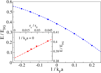
Figure 1: (color online) Energy per particle in the BEC-BCS crossover regime in units of $E_{FG}$ as a function of the scattering length $a$. The QMC points are the results of extrapolations to $r_{e}\rightarrow 0$ limit. In the inset we show the extrapolation at unitarity.

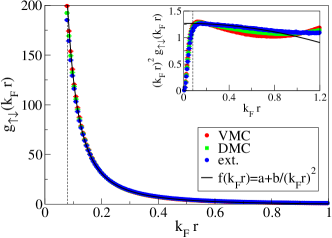
Figure 2: (color online) The calculated spin-opposite two-body distribution function at small distance $r$; the effective range of the interaction is $k_{F}\,r_{e}\approx 0.08$ (vertical black dashed line). The VMC (red), mixed (green) and extrapolated (blue) results are shown. The extrapolated QMC results are used to fit the function giving $b=1.2678$. In the inset we show the same functions multiplied by $(k_{F}r)^{2}$.

The variational wave function has been carefully optimized; in particular we optimize the pairing orbitals entering in the wave function by using VMC to minimize the energy Sorella:2001 . The fixed-node DMC energies do not depend on the Jastrow function $f_{J}$. Our simulations are performed with 66 particles in a periodic box, and we study the effect of the effective range of the interaction by changing $r_{e}$ and extrapolating to the $r_{e}\rightarrow 0$ limit. The results of 66 particles is very close to the infinite limit Forbes:2010 . Careful optimization of the variational wave function significantly improves the energy upper bounds. At unitarity, the best previous QMC results using 66 particles are $\xi=0.42(1)$ fixing $r_{e}/r_{0}\approx 0.08$ Carlson:2005 , and $\xi=0.42(1)$ using $r_{e}/r_{0}\approx 0.01$ Astrakharchik:2004 . Our new estimate is $\xi=0.4069(5)$ and $\xi=0.3923(4)$ with $r_{e}/r_{0}\approx 0.07$ and $0.02$ respectively. The parameters for $\phi$ at unitarity are $b=0.5k_{F}$, $d=5$ and the nonzero $a(k^{2})$ are given in Table 1.

$\frac{L^{2}}{4\pi^{2}}k^{2}$	$a(k^{2})$	$\frac{L^{2}}{4\pi^{2}}k^{2}$	$a(k^{2})$
0	0.00198	5	0.000190
1	0.00250	6	0.000200
2	0.00194	8	0.000167
3	0.00081	9	0.000163
4	0.00033	10	0.000120

Table 1: The optimized plane wave coefficients at unitarity for the pairing function.

Improved optimization of the trial wave function lowers the fixed-node energy by 4–7%. Careful extrapolation to $r_{e}\rightarrow 0$ limit is also important. We show an example at unitarity in the inset of Fig. 1 where we plot QMC points at different effective ranges, and their extrapolation. Using more points and a more complex fit typically provides a somewhat lower upper bound to the energy Forbes:2010 ; such a correction is about 0.002 to $\xi$.

We optimized the many–body wave function for systems with different scattering lengths and for each value of $k_{F}a$ we repeated the extrapolation of $r_{e}$. Our results of $\xi(k_{F}a)$ are shown in Fig. 1. Fitting the QMC points shown in Fig. 1 gives the values $\xi=0.383(1)$, $\zeta=0.901(2)$ and $\nu=0.49(2)$. Using Eq. 5 we predict

$$\frac{C}{k_{F}^{4}}=\frac{2\zeta}{5\pi}=0.1147(3)\,.$$ (10)

An alternative direct method for calculating the contact can be obtained by computing correlation functions at unitarity. For example, the pair distribution function is shown in Fig. 2, where we compare the VMC result with the mixed estimate computed with DMC. The two results are almost identical and differences appear only for very small distances. The value of $\zeta$ is obtained by fitting $g_{\uparrow\downarrow}(k_{F}r)$ in the range $r_{e}\ll r\ll k_{F}^{-1}$ using the function $a+b/r^{2}$. The fit gives $b=1.2678(1)$. Using Eqs. 2 and 5, gives the value for $\zeta=0.897(2)$ in good agreement with the result extracted from Eq. 6.

The calculated radial one-body density matrix $\rho^{(1)}(k_{F}r)$ is shown in Fig. 3 using VMC and the mixed DMC results. Again the results are nearly identical, with strikingly linear behavior over a large range of small $k_{F}r$ values. The fit gives $\zeta=0.895(16)$ again in good agreement with the equation of state result.

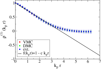
Figure 3: (color online) The radial one-body density matrix, symbols and $k_{F}\,r_{e}\approx 0.08$ as in Fig. 2. A line showing the linear fit with $c=0.2685$ is also shown, the dominant short-range behavior is accurate up to approximately $k_{F}r\sim 3$.

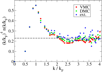
Figure 4: (color online) The calculated momentum distribution summed over both spins multiplied by $k^{4}/k_{F}^{4}$ showing the $k^{-4}$ tail. Dashed line show $2C/k_{F}^{4}$ of Eq. 10

The calculated momentum distribution is shown in Fig. 4. The momentum distribution and the one-body density matrix are each other’s Fourier transform. The only difference in our calculations are that the angular average has been done in real space for the one-body density matrix to give the radial one-body density matrix, while the momentum distribution is calculated for the $k$ vectors that correspond to the periodic simulation cell. The extraction of the $k^{4}$ tail is rather noisy; using the radial one-body density matrix gives a more accurate fit. From our results it appears that the contact term dominates the behavior for $k\gtrsim 2k_{F}$. Our asymptote is consistent with the value $0.229(1)$ expected from $\zeta=0.901(2)$ (dashed line in Fig. 4).

Recent experiments have measured the contact parameter from the equation of state Navon:2010 , momentum distribution directly using ballistic expansion and indirectly through the rf line shape and photoemission spectroscopy Stewart:2010 , and from the static structure factor Kuhnle:2010 . Navon et al. Navon:2010 extracted a value of $\zeta=0.93(5)$ from their equation of state measurements. Our best value of $\zeta=0.901(3)$ is well within their experimental errors. Kunhle et al. Kuhnle:2010 calculate a slope of $S(k)$ versus $k_{F}/k$ at large $k$ for $1/(k_{F}a)=0$ of $0.75(3)$ at $T=0.10(2)T_{F}$, giving a value of $\zeta=0.80(3)$, while Stewart et al. give values somewhat away from unitarity which also give $\zeta$ lower than our value.

In conclusion, we have used Quantum Monte Carlo techniques to study the short-range correlations of unitary Fermi gases as encoded in Tan’s contact parameter. The extractions from various observables all give the same result within statistical errors. These Monte Carlo methods give particularly low variance values for the energy of the system and with minimal bias. Therefore extracting the contact parameter from the equation of state is the simplest and most reliable. However, we have shown that its value extracted from the two-body radial distribution function, the one-body radial density matrix, and the momentum distribution also give the same results albeit with somewhat larger error bars. For each of these quantities we have also determined the regime over which the leading contact behavior is dominant, which should be useful to future experiment in extracting the contact behavior and leading corrections.

Acknowledgements: We thank J. E. Drut for valuable discussions. This work is supported by the U.S. Department of Energy, Office of Nuclear Physics, under contracts DE-FC02-07ER41457 (UNEDF SciDAC), and DE-AC52-06NA25396 and by the National Science Foundation grant PHY-0757703. KES thanks the Los Alamos National Laboratory and the New Mexico Consortium for their hospitality. Computer time was made available by Los Alamos Open Supercomputing.

References

- (1) S. Giorgini, L. P. Pitaevskii, and S. Stringari, Rev. Mod. Phys. 80, 1215 (2008)
- (2) J. Carlson and S. Reddy, Phys. Rev. Lett. 95, 060401 (2005)
- (3) J. Carlson and S. Reddy, Phys. Rev. Lett. 100, 150403 (2008)
- (4) A. Schirotzek, Y.-i. Shin, C. H. Schunck, and W. Ketterle, Phys. Rev. Lett. 101, 140403 (2008)
- (5) D. Lee, Phys. Rev. C 78, 024001 (2008)
- (6) S. Tan, Ann. Phys. 323, 2952 (2008)
- (7) S. Tan, Ann. Phys. 323, 2971 (2008)
- (8) S. Tan, Ann. Phys. 323, 2987 (2008)
- (9) E. Braaten(2010), arXiv:1008.2922
- (10) N. Navon, S. Nascimbène, F. Chevy, and C. Salomon, Science 328, 729 (2010)
- (11) E. D. Kuhnle, H. Hu, X.-J. Liu, P. Dyke, M. Mark, P. D. Drummond, P. Hannaford, and C. J. Vale, Phys. Rev. Lett. 105, 070402 (2010)
- (12) J. T. Stewart, J. P. Gaebler, T. E. Drake, and D. S. Jin, Phys. Rev. Lett. 104, 235301 (2010)
- (13) H. Hu, X.-J. Liu, and P. D. Drummond(2010), arXiv:1011.3845
- (14) C. Lobo, I. Carusotto, S. Giorgini, A. Recati, and S. Stringari, Phys. Rev. Lett. 97, 100405 (2006)
- (15) R. Combescot, S. Giorgini, and S. Stringari, Europhys. Lett. 75, 695 (2006)
- (16) J. E. Drut, T. A. Lähde, and T. Ten arXiv:1012.5474
- (17) S.-Q. Su, D. E. Sheehy, J. Moreno, and M. Jarrell, Phys. Rev. A 81, 051604 (May 2010)
- (18) T. Abe and R. Seki, Phys. Rev. C 79, 054003 (2009)
- (19) F. Palestini, A. Perali, P. Pieri, and G. C. Strinati, Phys. Rev. A 82, 021605 (2010)
- (20) J.-W. Chen and E. Nakano, Phys. Rev. A 75, 043620 (2007)
- (21) D. Lee, Eur. Phys. J. A 35, 171 (2008)
- (22) E. Braaten and L. Platter, Phys. Rev. Lett. 100, 205301 (2008)
- (23) R. Combescot, F. Alzetto, and X. Leyronas, Phys. Rev. A 79, 053640 (2009)
- (24) F. Werner, L. Tarruell, and Y. Castin, Eur. Phys. J. B 68, 401 (2009)
- (25) H. Hellmann, Einführung in die Quantenchemie (Leipzig: Franz Deuticke, 1937) p. 285
- (26) R. P. Feynman, Phys. Rev. 56, 340 (1939)
- (27) Some authors define the contact as an extensive quantity , where is the volume, and report the unitless intensive quantity .
- (28) J. Carlson, S.-Y. Chang, V. R. Pandharipande, and K. E. Schmidt, Phys. Rev. Lett. 91, 050401 (2003)
- (29) S. Y. Chang, V. R. Pandharipande, J. Carlson, and K. E. Schmidt, Phys. Rev. A 70, 043602 (2004)
- (30) A. Gezerlis, S. Gandolfi, K. E. Schmidt, and J. Carlson, Phys. Rev. Lett. 103, 060403 (2009)
- (31) S. Sorella, Phys. Rev. B 64, 024512 (2001)
- (32) M. McNeil Forbes, S. Gandolfi, and A. Gezerlis(2010), arXiv:1011.2197
- (33) G. E. Astrakharchik, J. Boronat, J. Casulleras, and S. Giorgini, Phys. Rev. Lett. 93, 200404 (2004)