Dynamics and morphology of dendritic flux avalanches in superconducting films

Abstract

We develop a fast numerical procedure for analysis of nonlinear and nonlocal electrodynamics of type-II superconducting films in transverse magnetic fields coupled with heat diffusion. Using this procedure we explore stability of such films with respect to dendritic flux avalanches. The calculated flux patterns are very close to experimental magneto-optical images of MgB₂ and other superconductors, where the avalanche sizes and their morphology change dramatically with temperature. Moreover, we find the values of a threshold magnetic field which agrees with both experiments and linear stability analysis. The simulations predict the temperature rise during an avalanche, where for a short time $T\approx 1.5T_{c}$, and a precursor stage with large thermal fluctuations.

I Introduction

The gradual penetration of magnetic flux in type-II superconductors subjected to an increasing applied field or electrical current can be interrupted by dramatic avalanches in the vortex matter.Altshuler and Johansen (2004) The mechanism responsible for the avalanches is that an initial fluctuation reduces locally the pinning of some vortices, which start to move, thus creating dissipation followed by depinning of even more vortices. A positive feedback loop is formed where a small perturbation can escalate into a macroscopic thermomagnetic breakdown.Mints and Rakhmanov (1981)

In thin film superconductors, the dynamics and morphology of these avalanches is tantalizing, when at very high speeds they develop into complex dendritic structures, which once formed remain robust against changes in external conditions. When repeating identical experiments one finds that the patterns are never the same although qualitative features of the morphology, such as the degree of branching and overall size of the structure, show systematic dependences on, e.g., temperature. Using magneto-optical imaging flux avalanches with these characteristics have been observed in films of Nb, Durán et al. (1995); *welling04 YBa₂Cu₃O_7-x, P. Brüll et al. (1992); *leiderer93; *bolz03 MgB₂, Johansen et al. (2002); Albrecht et al. (2005); *olsen07 Nb₃Sn, Rudnev et al. (2003) YNi₂B₂C, Wimbush et al. (2004) and NbN. Rudnev et al. (2005); *yurchenko07 Investigations of onset conditions for the avalanche activity have identified material dependent threshold values in temperature, Johansen et al. (2002) applied magnetic field, Barkov et al. (2003); Yurchenko et al. (2007) and transport current, Bobyl et al. (2002) as well as in sample size.Denisov et al. (2006a) Analytical modeling of the nucleation stage has explained many of these thresholds using linear stability analysis.Rakhmanov et al. (2004); Aranson et al. (2005); Denisov et al. (2006b, a)

Far from being understood is the development of the instability from its nucleation stage to the fully developed dendritic pattern. Aranson et al.Aranson et al. (2005) explored the dynamics of the flux avalanches as a numerical solution of Maxwell’s equations with temperature dependent critical current density. The dynamical process was governed by the interplay between an extremely nonlinear current-voltage relation, heat diffusion, and the nonlocal electrodynamics characteristic for thin superconducting films. To treat the nonlocal electrodynamics the authors used periodic continuation of the sample taken as an infinite strip. This scheme should be a good approximation inside the sample, although not necessarily close to the edges. In fact, in thin films the magnetic field near the edges is significantly enhanced Brandt and Indenbom (1993); *zeldov94 due to the flux expulsion. Moreover, all experiments show that the instability is always nucleated at an edge. Therefore, a careful account of the electrodynamics close to the edges, including the regions outside the film, is expected to be crucially important.Brandt (1995a)

In this work we study the formation and characteristics of dendritic flux avalanches using a numerical scheme that takes into account the nonlocal electrodynamics both inside and outside a finite-sized superconducting film. It is shown that our simulations largely reproduces experimental results obtained by magneto-optical imaging of dendritic avalanches in films of MgB₂, and furthermore gives detailed insight into not yet observed quantities such as local temperature rise and electrical field.

The paper is organized as follows. Section II presents the model and the equations describing the process. The numerical scheme including the implementation of boundary conditions and thermomagnetic feedback is described in Sec. III. The results for the time-dependent distributions of magnetic flux and temperature are presented and discussed in Sec. IV, while Sec. V gives the conclusions.

II Model

Consider a rectangular superconducting film zero-field cooled below the critical temperature, $T_{c}$, followed by a gradual increase in a perpendicular applied magnetic field. The film is deposited on a substrate, which in the process will be regarded as a sink for the dissipated heat. Shown in Fig. 1 is a sketch of the overall configuration, including the relevant fields and currents.

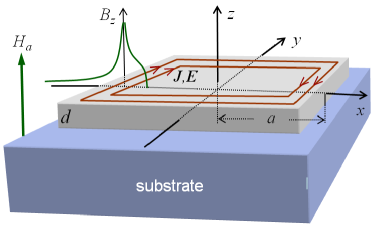
Figure 1: (Color online) Schematic of the sample configuration.

The macroscopic behavior of type-II superconductor films in a transverse applied magnetic field, $H_{a}$, is well described by quasi-static classical electrodynamics. Brandt (1995b, a) Here the sharp depinning of vortices under flowing current is represented by a highly nonlinear current-voltage relation

$$\mathbf{E} = \rho(J)\mathbf{J}/d\,,$$

$$\rho(J) \equiv \left\{\begin{array}[]{lll}\rho_{0}\left(J/J_{c}\right)^{n-1},&J\leq J_{c},&T\leq T_{c}\,,\\ \rho_{0}\,,&J>J_{c},&T\leq T_{c}\,,\\ \rho_{n}\,,&&T>T_{c}\,.\end{array}\right.$$ (4)

Here $\mathbf{E}$ is the electric field, $\mathbf{J}$ is the sheet current ($J\equiv|\mathbf{J}|$), $J_{c}$ the critical sheet current, $n$ is the creep exponent, $\rho_{0}$ is a resistivity constant, $\rho_{n}$ is the normal resitivity, and $T$ is temperature. It is assumed that the sample thickness, $d$, is so small that variations in all relevant quantities across the thickness can be ignored. For $T\leq T_{c}$ the temperature dependence of the critical current and flux creep exponent Denisov et al. (2006a) are taken as

$$J_{c}=J_{c0}(1-T/T_{c})\ \ {\rm and}\ \quad n-1=n_{0}T_{c}/T\,,$$ (5)

where $J_{c0}$ and $n_{0}$ are constants.

The distribution of temperature is described by the heat diffusion equation

$$dc\,\dot{T}=d\nabla\cdot(\kappa\nabla T)-h(T-T_{0})+\mathbf{J}\cdot\mathbf{E}\,,$$ (6)

where $\kappa$ is the thermal conductivity of the superconductor, $c$ is its specific heat, $T_{0}$ is the substrate temperature, taken to be constant, and $h$ is the coefficient of heat transfer between the film and the substrate. The $\kappa,c$ and $h$ are all assumed to be proportional to $T^{3}$, whereas a relatively weak temperature dependences of $\rho_{0}$ and $\rho_{n}$ are neglected. Schneider et al. (2001); Denisov et al. (2006a)

Following Ref. Brandt, 1995a we define the local magnetization, $g=g(\mathbf{r})$, as

$$\nabla g\times\mathbf{z}=\nabla\times(g\mathbf{z})=\mathbf{J}\ ,$$ (7)

where $\mathbf{r}\equiv(x,y)$ is a 2D vector in the film plane, and $\mathbf{z}$ is the unit vector in the perpendicular direction. Outside the sample there are no currents, and we set $g=0$ by definition. The Biot-Savart law can then be written as

$$\frac{B_{z}(\mathbf{r})}{\mu_{0}}-H_{a}=\hat{Q}g\equiv\int d^{2}r^{\prime}\,Q(\mathbf{r}-\mathbf{r}^{\prime},z)g(\mathbf{r}^{\prime})\,,$$ (8)

where the integral is calculated over the whole plane. The kernel $Q(\mathbf{r})$ should be calculated as a limit at $z\to 0$ of the expression

$$Q(\mathbf{r},z)=\frac{1}{4\pi}\frac{2z^{2}-r^{2}}{(z^{2}+r^{2})^{5/2}}\,,\ r\equiv|\mathbf{r}|\,.$$ (9)

Here reqularization is needed to avoid formal divergence of the r.h.s. of Eq. (8) at $z=0$, $\mathbf{r}=\mathbf{r}^{\prime}$. The Fourier transform of $\lim_{z\to 0}Q(\mathbf{r},z)$ is equal to $k/2$.Roth et al. (1989) Therefore, from the convolution theorem it follows that the inverse operator $\hat{Q}^{-1}$ acting on some function $\varphi(\mathbf{r})$ can be expressed as

$$\hat{Q}^{-1}\varphi(\mathbf{r})=2\mathcal{F}^{-1}\left(k^{-1}\mathcal{F}[\varphi(\mathbf{r})]\right)\,.$$ (10)

Here ${\mathcal{F}}[\varphi(\mathbf{r})]$ and ${\mathcal{F}}^{-1}[\varphi(\mathbf{k})]$ are Fourier and inverse Fourier transform, respectively, and $k\equiv|\mathbf{k}|$.

Inverting Eq. (8) one arrives at the equation for the time evolution of the local magnetization,

$$\dot{g}(\mathbf{r},t)=2\mathcal{F}^{-1}\left(k^{-1}\mathcal{F}\left[\mu_{0}^{-1}\dot{B}_{z}(\mathbf{r},t)-\dot{H}_{a}(t)\right]\right)\,.$$ (11)

Equations (6), (7) and (11) therefore determine the dynamics of $g(\mathbf{r},t)$, $T(\mathbf{r},t)$, etc. To solve these equations numerically we proceed from the continuous to a discrete formulation.

III Numerical approach

To allow use of the fast Fourier transform (FFT) we consider a rectangular area of size $2L_{x}\times 2L_{y}$ containing the sample plus a substantial part of its surrounding area. A key point is to select proper values for $L_{x}$ and $L_{y}$ relative to the sample size, $2a\times 2b$. By including too little area outside the sample one clips away the slowly decaying tail of the stray fields, leading to decreased accuracy at large scales, and major deviations from the correct physical behavior. Brandt (1995a) On the other hand, including too much of the outside area keeping the same number of the grid points tends to decrease the accuracy at small scales, where actually the most interesting features of the dendritic avalanches appear. This blurring can be compensated by using a finer spatial grid, at the cost of a rapidly increasing computation time.

A careful test of our numerical scheme was done by comparing the calculations with the exact solution for the Bean critical state in an infinitely long strip. Brandt and Indenbom (1993); *zeldov94 It is found that already with $L_{x}/a\gtrsim 1.3$ the calculated results are correct within a few percent, and are essentially indistinguishable from the exact solution in graphic comparisons.

In the FFT-based calculations the rectangle $2L_{x}\times 2L_{y}$ is discretized as a $N_{x}\times N_{y}$ equidistant grid, and used as unit cell in an infinite superlattice. The Fourier wave vectors $k_{x,y}$ are then discrete, $k_{x,y}=\pi q_{x,y}/L_{x,y}$, where $q_{x,y}$ are integers. The Brillouin zone is chosen as $|q_{x,y}|\leq N_{x,y}/2$, which ensures $g(\mathbf{r},t)$, $T(\mathbf{r},t)$, etc. to be real valued.

The calculation of the temporal evolution is based on a discrete integration forward in time of the local magnetization

$$g(\mathbf{r},t+\Delta t)\approx g(\mathbf{r},t)+\Delta t~{}\dot{g}(\mathbf{r},t)\,,$$ (12)

starting from $g(\mathbf{r},0)=0$. Once $g(\mathbf{r},t)$ is known at time $t$, we proceed one time step by determining $\dot{g}(\mathbf{r},t)$. The $\dot{g}(\mathbf{r},t)$ can be calculated from Eq. (11), provided $\dot{B}_{z}$ is known everywhere within the unit cell. For this, we have to find self-consistent solutions for $\dot{g}$ and $\dot{B}_{z}$ given the function $g$.

For the area inside the superconductor the material law, Eq. (II), applies and together with the Faraday law, $\dot{B_{z}}=-(\nabla\times\mathbf{E})_{z}$, it follows that

$$\dot{B}_{z}=\nabla\cdot(\rho\nabla g)/d\,.$$ (13)

The gradient $\nabla g(\mathbf{r},t)$ is readily calculated, and since the result allows finding $\mathbf{J}(\mathbf{r},t)$, from Eq. (7), also $\rho(\mathbf{r},t)$ is determined from Eq. (II). The difficult point is that $\dot{g}$ depends on the distribution of $\dot{B}_{z}$ in the whole unit cell. The task is to find the $\dot{B}_{z}$ outside the sample which leads to $\dot{g}=0$ outside. This cannot be calculated directly since there is a nonlocal relation between $\dot{B}_{z}$ and $\dot{g}$. Instead we use an iterative procedure.

Let us label the iterations by a superscript $(i)$. At the first step, $i=1$, we calculate $\dot{B}_{z}$ inside the superconductor from Eq. (13). Then an initial guess is made for the time derivative, $\dot{B}_{z}^{(1)}$, outside the sample. From Eq. (11) we now compute the time derivative $\dot{g}^{(1)}$. In general, this $\dot{g}^{(1)}$ does not vanish outside the superconductor. To correct for this, a new and improved $\dot{B}_{z}$ is chosen as

$$\dot{B}_{z}^{(i+1)}=\dot{B}_{z}^{(i)}-\mu_{0}\hat{Q}\hat{O}\dot{g}^{(i)}+C^{(i)},$$ (14)

where the projection operator $\hat{O}$ vanishes inside the superconductor and equals to 1 outside it. The constant $C^{(i)}$ is determined by the flux conservation,

$$\int d^{2}r\,[\dot{B}_{z}^{(i+1)}(\mathbf{r},t)-\mu_{0}\dot{H}_{a}]=0.$$ (15)

The procedure is stopped after $s$ iterations when the values of $\dot{g}$ outside the superconductor becomes sufficiently small. The final distribution, $\dot{g}^{(s)}(\mathbf{r})$, is taken as the “true” $\dot{g}(\mathbf{r},t)$, and substituted into Eq. (12) in order to advance in time.

A good choice for the initial state of the iteration at time $t$ is $\dot{B}_{z}^{(1)}(t)=\dot{B}_{z}^{(s)}(t-\Delta t)$, i.e., each iteration starts from the final distributions achieved during the previous iteration. Normally, $s=5$ iterations is sufficient to give good results.

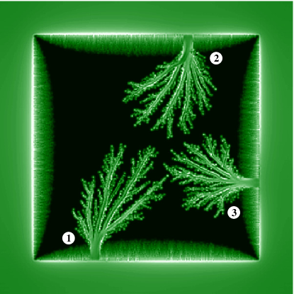
Figure 2: (Color online) Calculated distribution of $B_{z}$ at an applied field $H_{a}=0.18J_{c0}$, and substrate temperature $T_{0}=T_{c}/4$. The image brightness represents the magnitude of $B_{z}$. The sample contour appears as a bright rim of enhanced field, and the black central area is the flux-free Meissner state region.

IV Results and discussion

Numerical simulations were performed for samples shaped as a square of side $2a$ and with an outside area corresponding to $L_{x}=L_{y}=1.3a$. The total area is discretized on a 512$\times$512 equidistant grid. Quenched disorder is included in the model by a 10% reduction of $J_{c0}$ at randomly selected 5% of the grid points. The simulated flux penetration process starts at zero applied field with no flux trapped in the sample, which has a uniform temperature $T_{0}$.

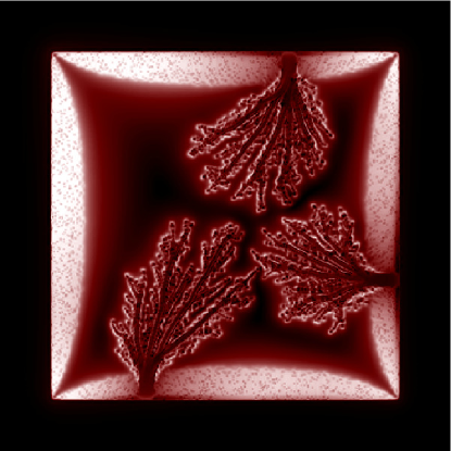
Figure 3: (Color online) Map of the sheet current, $J$, corresponding the image in Fig. 2. The brightness represents $J$, where black means $J=0$.

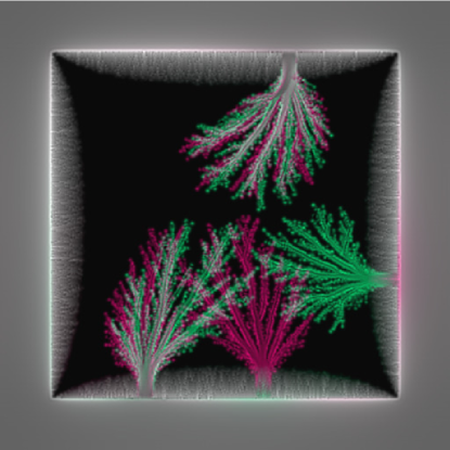
Figure 4: (Color online) Color-coded overlay of two separate runs with same quenched disorder but with different microscopic fluctuations. The pixels in gray-scale represent overlapping results. The parameters are the same as in the caption of Fig. 2.

Calculations were performed at $T_{0}=T_{c}/4$ using material parameters corresponding to a typical MgB₂ film,Schneider et al. (2001); Denisov et al. (2006a) $\rho_{n}$=7 $\mu\Omega$cm, $\kappa=0.17$ kW/Km$\times(T/T_{c})^{3}$ and $c=35$ kJ/Km${}^{3}\times(T/T_{c})^{3}$, where $\rho_{n}$ is the normal resistivity at $T_{c}=39~{}$K, $J_{c0}=50$ kA/m, $\rho_{0}=\rho_{n}$, $d=0.5~{}\mu$m, $a=2.2~{}$mm, and $h=220$ kW/Km${}^{2}\times(T/T_{c})^{3}$. We choose $n_{0}=19$ and limit the creep exponent to $n(T)\leq n_{\text{max}}=59$. The field was ramped from $H_{a}=0$ at a constant rate, $\dot{H}_{a}=10^{-5}J_{c0}\rho_{n}/ad\mu_{0}$.

Figure 2 shows the $B_{z}$-distribution at $\mu_{0}H_{a}=0.18\mu_{0}J_{c0}=11$ mT, where three large dendritic structures have already been formed. The numerical labels indicate the order in which they appeared during the field ramp. The first event took place at the threshold applied field, $\mu_{0}H_{\rm th}=0.145\mu_{0}J_{c0}=9.1$ mT, which is in excellent agreement with measurements on MgB₂ films just below 10 K$\approx T_{c}/4$. At lower fields, the flux penetration was gradual and smooth, just as seen on the left edge of the sample, where the characteristic “pillow effect” for films in the critical state is very well reproduced. 

The dendritic avalanches all nucleate at the edges, and one by one they quickly develop into a branching structure that extends far beyond the critical-state front and deep into the Meissner state area. The trees are seen to have a morphology that strongly resembles the flux structures observed experimentally in many superconducting films. Leiderer et al. (1993); Bolz et al. (2003); Durán et al. (1995); Welling et al. (2004); Johansen et al. (2002); Albrecht et al. (2005); Olsen et al. (2007); Rudnev et al. (2003); Wimbush et al. (2004); Yurchenko et al. (2007) The simulations also reproduce the experimental finding that once a flux tree is formed, the entire dendritic structure remains unchanged as $H_{a}$ continues to increase. The supplementary material includes a VIDEO clip of the dynamical process, and shows striking resemblance with magneto-optical observations of the phenomenon.

Figure 3 shows the sheet current magnitude, $J$, corresponding to the flux distribution in Fig. 2. From this map it is clear that the dendrites completely interrupt the current flow in the critical state, and redirect it around the perimeter of the branching structure. This vast perturbation of the current has been demonstrated experimentally earlier using inversion of magneto-optical images. Laviano et al. (2004); *olsen06 Note that the critical state region contains dark pixels which are the randomly distributed sites of reduced $J_{c0}$.

To investigate reproducibility in the pattern formation, microscopic fluctuations were introduced by randomly alternating between right- and left-derivatives in the discrete differentiation. Due to the nonlinear form of Eq. (II) this procedure gives large local variations in the electrical field. Figure 4 shows an overlay of two simulation runs with different realizations of the microscopic fluctuations while keeping the same quenched disorder in $J_{c0}$. The two resulting images were colored so that adding them gives shades of gray where both coincide in pixel values. Clearly, the two runs gave different results as far as the dendritic pattern is concerned. Both produced three branching structures, where two are rooted at the same place and the third is at a different location. Even for those with overlap, there are parts of the structure that differ considerably, especially in the finer branches. In contrast, both the critical state and the Meissner state regions are essentially identical in the two runs. Note the color at the edge of the right hand side near the root of the green dendrite, which reflects that the growth of the flux structure drains the external field near the root. Moreover, the root of all the trees are not far from the middle of the sides. Both features are in full accordance with experiments.

Each dendritic avalanche is accompanied by a large local increase in temperature. Shown in Fig. 5a is a plot of the maximum temperature in the film during a field ramp with substrate kept at $T_{0}=T_{c}/4$. The spikes in the temperature rise as high as $1.5T_{c}$. The maximum temperature is found in the root region of the avalanche. The heating above $T_{c}$ is an interesting prediction; to our knowledge, the temperature of propagating avalanches has not been observed experimentally. At the same time, the result is consistent with the measured heating of uniform flux jumps in Nb foils Prozorov et al. (2006) and the magnetic field-induced damage in a YBa₂Cu₃O_7-x film during dendritic growth.P. Brüll et al. (1992)

Figure 5: Maximum temperature in the superconductor during an ascending field ramp at $T_{0}=T_{c}/4$. The panels (a)-(c) are successive magnifications of the first avalanche event.

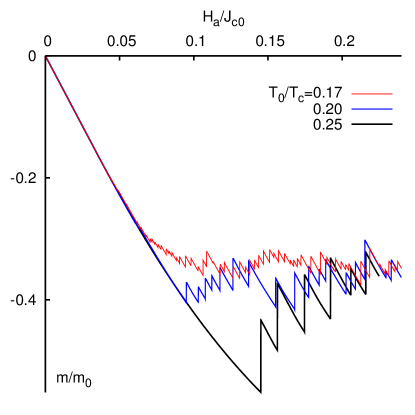
Figure 6: (Color online) Magnetic moment in units of $m_{0}=a^{3}J_{c0}$ as function of increasing field obtained by simulations at three different temperatures, $T_{0}$. Each jump in the curves represents a flux avalanche.

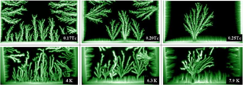
Figure 7: (Color online) Temperature variation in the morphology of flux dendrites. Top panels show simulated results for $B_{z}$ and bottom panels show magneto-optical images of a MgB₂ film.

The first avalanche in Fig. 5a appears at $H_{\rm th}=0.145J_{c0}$. Since the chosen disorder is rather weak and the ramp rate is high, the heat diffusion to the substrate is expectedly a more important stabilizing factor than lateral heat diffusion, the theoretically predicted threshold field is Denisov et al. (2006a)

$$H_{\text{th}}=\frac{J_{c}^{\prime}}{\pi}\tanh^{-1}\left(\frac{T_{c}h}{naJ_{c0}\mu_{0}\dot{H}_{a}}\right)\,.$$ (16)

At $T=T_{c}/4$ and with $n=59$ this gives $H_{\text{th}}=0.15J_{c0}$, in excellent agreement with the present simulation. Here, $J_{c}^{\prime}=0.6J_{c0}$ is the effective critical current, which is lower than $J_{c}$ due to flux creep. At the same time, the adiabatic threshold field Denisov et al. (2006b) is much smaller than $H_{\text{th}}$, which means that the heat diffusion and heat transfer to the substrate prevent avalanches. However, during short time intervals cooling is not always effective, and the temperature experiences large fluctuations. The fluctuations are particularly large as $H_{a}$ approaches triggering of an avalanche, see Fig. 5b. In these intervals both heat absorption and lateral heat diffusion play important roles in stabilizing the superconductor. A close-up view of the maximum temperature during the first avalanche at $T_{0}=T_{c}/4$ is shown in Fig. 5c. First, the temperature rapidly increases, and then decays much slower. The duration of the avalanche is $0.18~{}\mu$s. Since the length is $2.5~{}$mm, the average propagation velocity is of order $14$ km/s. This numerical value is reasonable compared to previous measurements, where the flux dendrites were triggered by a laser pulse in YBaCuO films.Leiderer et al. (1993); Bolz et al. (2003) The maximum electric field in the superconductor during the avalanche is also high, found from the simulations to be approximately $5$ kV/m.

The abrupt redirection of the current implies that the magnetic moment of the sample makes a jump and becomes smaller. Figure 6 shows the moment as function of the increasing applied field. Each vertical step corresponds to a flux avalanche. The lower curve, obtained for $T_{0}=T_{c}/4$, shows jumps with typical size of $0.1m_{0}$ with a slight dispersion, which is due to variations both in shape and location of the avalanches. More pronounced is the variation in jump size with temperature. As $T_{0}$ gets lower the jump size becomes smaller, and the events more frequent. In the graphs for $T_{0}/T_{c}=0.20$ and 0.17, the jump size reduces to $0.03m_{0}$ and $0.01m_{0}$, and jumps appear on average with field intervals of $\Delta H_{a}/J_{c0}=0.01$ and $0.002$, respectively. In real samples a similar temperature variation of jumps in the $m$-$H$ curves was observed by magnetometry. Zhao et al. (2002); Rudnev et al. (2003); Prozorov et al. (2006); Colauto et al. (2008)

It has been reported Johansen et al. (2002) that the morphology of flux avalanches is strongly temperature dependent. This is illustrated in the bottom panel of Fig. 7 showing three magneto-optical images of a 0.4 $\mu$m thick MgB₂ square film at $T_{0}=$4 K, 6.3 K and 7.9 K. The images show a crossover from many long fingers at 4 K to medium sized dendrites at 6.3 K, to a single highly branched structure at 7.9 K. The simulation results shown in the top panels reproduce this result and show exactly the same trend as the experiments. At the lowest temperature, $0.17T_{c}$, there are many finger-like avalanches. At the middle temperature $0.2T_{c}$ there are fewer avalanches, with typically three to four branches each. At the highest temperature $0.25T_{c}$ there is just one big avalanche, with seven main branches.

V Conclusion

In conclusion, we have developed and demonstrated the use of a fast numerical scheme for simulation of nonlinear and nonlocal transverse magnetic dynamics of type-II superconducting films under realistic boundary conditions. Our simulations of thermomagnetic flux avalanches qualitatively and quantitatively reproduces numerous experimentally observed features: the fast flux dynamics, morphology of the flux patterns, enhanced branching at higher temperatures, irreproducibility of the exact flux patterns, preferred locations for nucleation, and the existence of a threshold field. The scheme allows determination of key characteristics of the process such as maximal values of the temperature and electric field as well as typical propagation velocity.