Time-dependent bond-current functional theory for lattice Hamiltonians: fundamental theorem and application to electron transport

Abstract

The cornerstone of time-dependent (TD) density functional theory (DFT), the Runge-Gross theorem, proves a one-to-one correspondence between TD potentials and TD densities of continuum Hamiltonians. In all practical implementations, however, the basis set is discrete and the system is effectively described by a lattice Hamiltonian. We point out the difficulties of generalizing the Runge-Groos proof to the discrete case and thereby endorse the recently proposed TD bond-current functional theory (BCFT) as a viable alternative. TDBCFT is based on a one-to-one correspondence between TD Peierl’s phases and TD bond-currents of lattice systems. We apply the TDBCFT formalism to electronic transport through a simple interacting device weakly coupled to two biased non-interacting leads. We employ Kohn-Sham Peierl’s phases which are discontinuous functions of the density, a crucial property to describe Coulomb blockade. As shown by explicit time propagations, the discontinuity may prevent the biased system from ever reaching a steady state.

I Introduction

The central idea of time-dependent (TD) density functional theory (DFT) is to map a time-dependent and interacting many-particle system onto a time-dependent system of non-interacting particles moving in an effective Kohn-Sham (KS) potential, $v_{\rm KS}({\bf r},t)$, chosen such that the TD densities of the interacting and non-interacting systems are equal. From the knowledge of $v_{\rm KS}({\bf r},t)$ it is then possible to compute the TD density $n({\bf r},t)$, and hence the TD longitudinal current, in a one-particle manner. With this results as a starting point, an exact TDDFT formulation of quantum transport which can cope with both transient and steady-state regimes has been proposed StefanucciAlmbladh:04 ; KurthStefanucciAlmbladhRubioGross:05 .

The theoretical foundation for the aforementioned mapping is laid down by the celebrated Runge-Gross theorem RungeGross:84 whose essential statement is that the time evolution of two systems evolving from the same initial state $|\Psi_{0}\rangle$ under the influence of two different TD potentials $v({\bf r},t)$ and $v^{\prime}({\bf r},t)$, which are analytic in time and differ by more than a purely time-dependent, position-independent function $C(t)$, leads to different TD densities $n({\bf r},t)$ and $n^{\prime}({\bf r},t)$. This theorem was developed further by van Leeuwen Leeuwen:99 who showed that for a many-body system with a given particle-particle interaction $w(|{\bf r}-{\bf r}^{\prime}|)$ and moving in some TD potential $v({\bf r},t)$, the TD density can be reproduced in another many-body system with a different interaction $w^{\prime}(|{\bf r}-{\bf r}^{\prime}|)$ and moving in a TD potential $v^{\prime}({\bf r},t)$ provided that the initial states $|\Psi(0)\rangle$ and $|\Psi^{\prime}(0)\rangle$ of the two systems yield the same density and longitudinal current. Moreover, for a given initial state the potential $v^{\prime}({\bf r},t)$ is unique up to a purely time-dependent function. Recently, Ruggenthaler and van Leeuwen extended the validity of these results by relaxing the condition of Taylor-expandability in time rvl.2010 .

The van Leeuwen theorem reduces to the Runge-Gross theorem for $w=w^{\prime}$ and $|\Psi(0)\rangle=|\Psi^{\prime}(0)\rangle$, and establishes the existence of a non-interacting KS system for $w^{\prime}=0$ and $|\Psi^{\prime}(0)\rangle=|\Phi_{\rm KS}\rangle$ a Slater determinant. In this latter case the potential $v^{\prime}({\bf r},t)$ reproducing a given density becomes the Kohn-Sham (KS) potential $v_{\rm KS}({\bf r},t)$ of TDDFT. In general, the KS potential is uniquely determined by the time-dependent density $n({\bf r},t)$, and the initial states $|\Psi(0)\rangle$ and $|\Phi_{\rm KS}\rangle$. If we further assume that the initial states $|\Psi(0)\rangle$ and $|\Phi_{\rm KS}\rangle$ are ground states, then via the Hohenberg-Kohn HohenbergKohn:64 and Kohn-Sham KohnSham:65 theorems of static density functional theory both initial states are uniquely determined by the initial density $n({\bf r},0)$, and the KS potential $v_{\rm KS}({\bf r},t)$ becomes a unique functional of the density alone. The TD density can then be calculated from the TD KS equations RungeGross:84

$$i\frac{\partial}{\partial t}\varphi_{j}({\bf r},t)=\left(-\frac{\nabla^{2}}{2}+v_{\rm KS}[n]({\bf r},t)\right)\varphi_{j}({\bf r},t),$$ (1)

and

$$n({\bf r},t)=\sum_{j}^{\rm occ}|\varphi_{j}({\bf r},t)|^{2},$$ (2)

where the sum in Eq. (2) is over the occupied orbitals in the KS Slater determinant.

Generally, in practical implementations of the continuum TD KS equations there are three independent sources of errors: (i) the use of only a finite number of basis functions, i.e., a de facto description of the problem by a discrete or lattice Hamiltonian; (ii) the approximation employed for the exchange-correlation (XC) potential and (iii) inherent numerical inaccuracies. Even if we could use the exact KS potential (designed for continuum systems) and run the program on a machine with infinite accuracy, when using a finite basis set the densities of the KS system and of the original interacting system will, in general, differ. In fact, it would be useful to have a discrete version of TDDFT for ruling out the errors due to the incompleteness of the basis set. An even stronger motivation for constructing a discrete TDDFT is to have an alternative tool for the study of model systems like, e.g., the Anderson model, the Hubbard model, etc. Recent works have shown that not all densities can be represented by lattice Hamiltonians b.2008 . The breakdown of this $v$-representability is due to the fact that the rate of density change which can be supported on a given lattice is limited by the inverse of the hopping matrix elements LiUllrich:08 ; Verdozzi:08 . In the next section we point out an even more severe problem related to the difficulties of generalizing the Runge-Gross proof to discrete or lattice Hamiltonians and re-understand why the continuum formulation works from the “discrete perspective”. To overcome these difficulties a TD bond-current functional theory (BCFT) has recently been proposed StefanucciPerfettoCini:10 ; here the underlying idea is to use the so called Peierls phases (discrete version of the vector potential) instead of the scalar potential as the basic KS field. We will present the TDBCFT and demonstrate the analogous of the van Leeuwen theorem in discrete systems. In Section III we take advantage of the TDBCFT formulation to construct a TD framework for quantum transport in model Hamiltonians. As an application in Section IV we will revisit the Coulomb Blockade (CB) phenomenon in the light of a recent finding on the relevance of the derivative discontinuity of static DFT functionals PerdewParrLevyBalduz:82 in the CB regime KurthStefanucciKhosraviVerdozziGross:10 . Conclusions and future perspectives are drawn in Section V.

II Time-dependent density functional theory on a lattice

II.1 Problems in generalizing Runge-Gross proof

We write the Hamiltonian of interacting electrons in some orthonormal basis $\varphi_{m}({\bf r})$ of orbitals localized at site $m$ by expanding the field operators as $\hat{\psi}_{\sigma}({\bf r})=\sum_{m}\hat{c}_{m\sigma}\varphi_{m}({\bf r})$, where the creation (annihilation) operators $\hat{c}_{m\sigma}^{\dagger}$ ($\hat{c}_{m\sigma}$) satisfy the anticommutation relations

$$\left\{\hat{c}_{m\sigma},\hat{c}_{n\sigma^{\prime}}^{\dagger}\right\}=\delta_{nm}\delta_{\sigma\sigma^{\prime}}\;.$$ (3)

For electrons exposed to a TD on-site potential $v_{m}(t)$, the Hamiltonian then reads

$$\hat{H}(t)=\hat{K}_{0}+\hat{V}(t)+\hat{H}_{\rm int},$$ (4)

where the non-interacting part consists of a static part

$$\hat{K}_{0}=\sum_{m,n}\sum_{\sigma}T_{mn}\hat{c}_{m\sigma}^{\dagger}\hat{c}_{n\sigma}$$ (5)

and a time-dependent external potential

$$\hat{V}(t)=\sum_{m}\sum_{\sigma}v_{m}(t)\hat{c}_{m\sigma}^{\dagger}\hat{c}_{m\sigma}\;.$$ (6)

where we assume that $v_{m}(t)=0$ for all times $t<0$. $\hat{H}_{\rm int}$ denotes the operator describing the electron-electron interaction. Note that $v_{m}(t)$ is coupled to the density operator $\hat{n}_{m}=\sum_{\sigma}\hat{c}_{n\sigma}^{\dagger}\hat{c}_{n\sigma}$ at site $m$.

In order to have a theoretical foundation for TDDFT on a lattice, one first has to prove the existence of a unique mapping between the expectation value $n_{m}(t)$ of the density operator at site $m$ and the on-site potential $v_{m}(t)$. The obvious idea is to adapt the original Runge-Gross proof RungeGross:84 for continuum Hamiltonians to the case of lattice Hamiltonians. However, this strategy runs into problems as we will now demonstrate.

Let $|\Psi(t)\rangle$ be the many-body state that solves the TD Schrödinger equation

$$i\frac{d}{dt}|\Psi(t)\rangle=\hat{H}(t)|\Psi(t)\rangle$$ (7)

with the initial condition $|\Psi(t=0)\rangle=|\Psi_{0}\rangle$. Then the expectation value $O(t)=\langle\hat{O}(t)\rangle=\langle\Psi(t)|\hat{O}(t)|\Psi(t)\rangle$ of any quantum mechanical operator $\hat{O}(t)$ satisfies the equation of motion

$$\frac{\rm d}{{\rm d}t}O(t)=\left\langle\frac{\partial\hat{O}(t)}{\partial t}\right\rangle+i\left\langle[\hat{H}(t),\hat{O}(t)]\right\rangle\;.$$ (8)

For a straightforward generalization of the Runge-Gross proof to lattice systems one needs to show that two wavefunctions $|\Psi(t)\rangle$ and $|\Psi^{\prime}(t)\rangle$ which evolve under the influence of two different potentials $v_{m}(t)\neq v^{\prime}_{m}(t)$ from the same initial state $|\Psi(0)\rangle=|\Psi^{\prime}(0)\rangle=|\Psi_{0}\rangle$ always lead to different TD densities $n_{m}(t)\neq n^{\prime}_{m}(t)$. Let us, for simplicity, consider the simplest case of two time-independent potentials $v_{m}$ and $v^{\prime}_{m}$ that differ by more than an additive constant. To show that they generate two different TD densities we calculate the succesive time-derivatives in $t=0$ of $n_{m}(t)$ and $n^{\prime}_{m}(t)$ until the order (if any) at which they differ. The zero-th and first derivatives in $t=0$ are clearly the same. From Eq. (8) the second derivative of $n_{m}(t)$ and $n^{\prime}_{m}(t)$ in $t=0$ reads

$$\ddot{n}_{m}(0)=\sum_{k}(T_{mk}\rho_{km}+\rho_{mk}T_{km})(v_{k}-v_{m})+\Delta_{m},$$ (9)

$$\ddot{n}^{\prime}_{m}(0)=\sum_{k}(T_{mk}\rho_{km}+\rho_{mk}T_{km})(v^{\prime}_{k}-v^{\prime}_{m})+\Delta_{m},$$ (10)

with $\rho_{mk}=\sum_{\sigma}\langle\Psi_{0}|\hat{c}^{\dagger}_{k\sigma}\hat{c}_{m\sigma}|\Psi_{0}\rangle$ the one-particle density matrix at $t=0$ and

$$\Delta_{m} = -\Big{\langle}\Psi_{0}\Big{|}\,\left[\hat{K}_{0},[\hat{K}_{0},\hat{n}_{m}]\right]\Big{|}\Psi_{0}\Big{\rangle}$$ (11)

$$-\Big{\langle}\Psi_{0}\Big{|}\left[\hat{H}_{\rm int},[\hat{H}_{\rm int},\hat{n}_{m}]\right]\Big{|}\Psi_{0}\Big{\rangle}\;.$$

Introducing the short-hand notation $K_{mk}=T_{mk}\rho_{km}+\rho_{mk}T_{km}$ for the kinetic energy density of the bond $k-m$, the difference $\delta\ddot{n}=\ddot{n}(0)-\ddot{n}^{\prime}(0)$ is simply given by the formula below

$$\delta\ddot{n}_{m}=\sum_{k}K_{mk}(\delta v_{k}-\delta v_{m}),$$ (12)

where $\delta v=v-v^{\prime}$. Like in the original Runge-Gross proof we now proceed by reductio ad absurdum. Assume that $\delta\ddot{n}$ vanishes for a non-vanishing (and non-constant) $\delta v$. Then, multiplying both sides of Eq. (12) by $\delta v_{m}$ and summing over $m$ we find

$$0=\frac{1}{2}\sum_{km}K_{mk}(\delta v_{k}-\delta v_{m})^{2},$$ (13)

where we made use of the symmetry $K_{mk}=K_{km}$. Due to the fact that the $K_{mk}$ do not have a definite sign Eq. (13) is not an absurdum. In fact, in a lattice theory we could have two different potentials that yield the same second derivative of the density in $t=0$. We should then proceed further and try to prove that the third derivatives are different. One immediately realizes, however, that this way does not lead anywhere. There exist several counterexamples to the existence of a one-to-one correspondence between densities and potentials in a lattice Hamiltonian. Consider, for example, a one-dimensional ring with four sites, zero on-site energies $T_{mm}=0$ and nearest-neighbor hopping $T_{12}=T_{23}+T_{34}=T_{41}=T$, see Fig. 1. The single-particle state with amplitudes $\varphi(1)=1$, $\varphi(3)=-1$ and $\varphi(2)=\varphi(4)=0$ is an eigenstate with energy zero. Any external potential $v_{m}(t)$ with $v_{1}(t)=v_{3}(t)=0$ leaves the density unchanged.

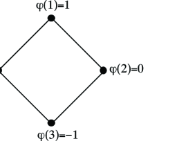
Figure 1: The 4-site ring described in the main text with a single-particle eigenstate of energy zero. Any external potential $v_{m}(t)$ with $v_{1}(t)=v_{3}(t)=0$ leaves the density unchanged.

In the next Section we show how to overcome these difficulties by considering the Peierls phases instead of the on-site potentials as the basic KS fields. Before, however, we find particularly instructive to re-understand why the continuum formulation works starting from the “discrete” perspective. To limit the complications we will focus on one-dimensional systems. Let $m=0,\pm 1,\pm 2,\ldots$ be the label of a grid point $x_{m}=m\Delta_{x}$ of a one-dimensional grid with lattice spacing $\Delta_{x}$. Choosing the $T_{mn}$ such that it gives the three-point discretization of the (continuum) kinetic energy

$$T_{mn}=-\frac{1}{2\Delta_{x}^{2}}\left(\delta_{m,n+1}-2\delta_{m,n}+\delta_{m,n-1}\right),$$ (14)

it is easy to show that the non-interacting Hamiltonian $\hat{H}_{0}(t)=\hat{K}_{0}+\hat{V}(t)$ (see Eqs. (5) and (6)) approaches the continuum Hamiltonian

$$\lim_{\Delta_{x}\to 0}\hat{H}_{0}(t)=\int dx\;\hat{\psi}^{{\dagger}}(x)\left[-\frac{\nabla^{2}}{2}+v(x,t)\right]\hat{\psi}(x),$$ (15)

where we defined the field operators

$$\hat{\psi}(x_{m})=\lim_{\Delta_{x}\rightarrow 0}\frac{\hat{c}_{m}}{\sqrt{\Delta_{x}}}\;,$$ (16)

and the scalar potential $v(x_{m},t)=v_{m}(t)$. Inserting the $T_{mn}$ of Eq. (14) into Eq. (13) and taking the limit $\Delta_{x}\to 0$ we find

$$0 = \lim_{\Delta_{x}\to 0}\Delta_{x}\sum_{k}{\rm Re}\left[\frac{\rho_{kk+1}}{\Delta_{x}}\right]\left(\frac{\delta v_{k+1}-\delta v_{k}}{\Delta_{x}}\right)^{2}$$ (17)

$$= \int dx\;n(x)\left(\frac{d}{dx}\;\delta v(x)\right)^{2},$$

with $n(x)=\lim_{\Delta_{x}\to 0}{\rm Re}\left[\frac{\rho_{kk+1}}{\Delta_{x}}\right]\geq 0$ the continuum density. For all situations of physical interest the integrand may vanish at most in a set of zero measure and is otherwise larger than zero. Thus, in the continuum case the above equation is an absurdum, in agreement with the Runge-Gross theorem.

II.2 TDCDFT on a lattice

The problems in extending the Runge-Gross theorem to lattice systems sketched in the previous Section can be circumvented by using TD Peierls phases instead of TD on-site potentials StefanucciPerfettoCini:10 . For arbitrary TD electromagnetic fields described by a scalar and vector potential $\tilde{v}({\bf r},t)$ and $\tilde{{\bf A}}({\bf r},t)$ one can always perform a gauge transformation such that $\tilde{v}({\bf r},t)\to v({\bf r})$ and $\tilde{{\bf A}}({\bf r},t)\to{\bf A}({\bf r},t)$, so that the time-dependence resides only in the vector potential. In particular, for those situations when there is only a TD potential $\tilde{v}({\bf r},t)$, we could always gauge $\tilde{v}$ away and work with a TD vector potential ${\bf A}({\bf r},t)$. In the localized basis we choose, therefore, the time-dependent Hamiltonian to have the form

$$\hat{H}(t)=\hat{K}(t)+\hat{H}_{\rm int},$$ (18)

where

$$\hat{K}(t)=\sum_{m,n}\sum_{\sigma}T_{mn}e^{i\gamma_{mn}(t)}\hat{c}_{m\sigma}^{\dagger}\hat{c}_{n\sigma},$$ (19)

and the time-dependence only resides in the Peierls phases $\gamma_{mn}(t)=-\gamma_{nm}(t)$. In a grid basis with grid points ${\bf r}_{m}$, the on-site matrix elements $T_{mm}=v({\bf r}_{m})$ contain information on the on-site electrostatic potential $v({\bf r})$ while the phases $\gamma_{mn}(t)=\frac{1}{c}\int_{{\bf r}_{m}}^{{\bf r}_{n}}d{\bf l}\cdot{\bf A}({\bf r},t)$ describe the effects of an external TD vector potential ${\bf A}({\bf r},t)$.

From Eq. (8) the density at site $m$ satisfies the equation of motion

$$\frac{\rm d}{{\rm d}t}n_{m}(t)=\sum_{n}J_{mn}(t)+i\left\langle[\hat{H}_{\rm int},\hat{n}_{m}]\right\rangle$$ (20)

where we have defined the bond-current operator $\hat{J}_{mn}(t)$ according to

$$\hat{J}_{mn}(t)=\frac{1}{i}\sum_{\sigma}\left(T_{mn}e^{i\gamma_{mn}(t)}\hat{c}^{\dagger}_{m\sigma}\hat{c}_{n\sigma}-{\rm H.c.}\right)\;.$$ (21)

In turn, the equation of motion for $J_{mn}(t)$ reads

$$\frac{\rm d}{{\rm d}t}J_{mn}(t)=K_{mn}(t)\frac{\rm d}{{\rm d}t}\gamma_{mn}(t)+F_{mn}(t)$$ (22)

with the “kinetic energy” density operator

$$\hat{K}_{mn}(t)=\sum_{\sigma}\left(T_{mn}e^{i\gamma_{mn}(t)}\hat{c}_{m\sigma}^{\dagger}\hat{c}_{n\sigma}+{\rm H.c.}\right)$$ (23)

and

$$\hat{F}_{mn}(t)=i[\hat{H}(t),\hat{J}_{mn}(t)]\;.$$ (24)

We now ask the question whether the bond-currents $J_{mn}(t)$ along those bonds with $T_{mn}\neq 0$ can be reproduced by another Hamiltonian $\hat{H}^{\prime}(t)$ with a different interaction and a different TD electromagnetic field, i.e.,

$$\hat{H}^{\prime}(t)=\hat{K}^{\prime}(t)+\hat{H}^{\prime}_{\rm int}$$ (25)

with

$$\hat{K}^{\prime}(t)=\sum_{m,n}T_{mn}e^{i\gamma^{\prime}_{mn}(t)}\hat{c}_{m\sigma}^{\dagger}\hat{c}_{n\sigma}\;.$$ (26)

Note that the matrix elements $T_{mn}$ in Eq. (26) are the same as in Eq. (19). Let us define the initial configuration of the primed system as the couple $\{|\Psi_{0}^{\prime}\rangle,\gamma^{\prime}(0)\}$, that consists of the initial state and the initial value of the Peierls phases. For the current $J^{\prime}_{mn}(t)$ of the primed system to be the same as the current $J_{mn}(t)$ at the initial time $t=0$, the initial configuration must be compatible, i.e., it must fulfill

$$\langle\Psi^{\prime}_{0}|\frac{1}{i}\sum_{\sigma}\left(T_{mn}e^{i\gamma^{\prime}_{mn}(0)}\hat{c}^{\dagger}_{m\sigma}\hat{c}_{n\sigma}-{\rm H.c.}\right)|\Psi^{\prime}_{0}\rangle=J_{mn}(0).$$ (27)

Assuming the existence of at least one compatible configuration we demonstrate below that there exist TD Peierls phases $\{\gamma^{\prime}(t)\}$ for which $J_{mn}(t)=J^{\prime}_{mn}(t)$ for all bonds with $T_{mn}(0)\neq 0$, and that these phases are unique.

The bond current densities $J_{mn}(t)$ and $J^{\prime}_{mn}(t)$ of the two systems are the same provided that

$$K^{\prime}_{mn}(t)\frac{\rm d}{{\rm d}t}\gamma^{\prime}_{mn}(t)=K_{mn}(t)\frac{\rm d}{{\rm d}t}\gamma_{mn}(t)+F_{mn}(t)-F^{\prime}_{mn}(t)\;.$$ (28)

To proceed further we adopt the same strategy of Vignale Vignale:04 in the context of TD current DFT, and expand all quantities in Eq. (28) in a Taylor series around $t=0$, e.g.,

$$K^{\prime}_{mn}(t)=\sum_{l=0}^{\infty}K_{mn}^{\prime(l)}\;t^{l}\;.$$ (29)

Inserting the Taylor expansions into Eq. (28) and equating the coefficients with power $l$ then gives

$$K_{mn}^{\prime(0)}(l+1)\gamma_{mn}^{\prime(l+1)}=-\sum_{k=0}^{l-1}(k+1)K_{mn}^{\prime(l-k)}\gamma_{mn}^{\prime(k+1)}$$ (30)

$$+\sum_{k=0}^{l}(k+1)K_{mn}^{(l-k)}\gamma_{mn}^{(k+1)}+F_{mn}^{(l)}-F_{mn}^{\prime(l)}\;.$$

The quantities $K^{\prime}_{mn}(t)$ and $F^{\prime}_{mn}(t)$ depend explicitly on the phases $\{\gamma^{\prime}(t)\}$ and therefore their $l$-th derivative depend on all the $k$-th derivatives $\{\gamma^{\prime(k)}\}$ with $k\leq l$. Thus, under the mild condition that the initial compatible configuration is chosen in such a way that

$$K^{\prime}_{mn}(0)=K_{mn}^{\prime(0)}\neq 0\;,$$ (31)

Eq. (30) constitute a system of recursive relations to determine all Taylor coefficients of $\gamma^{\prime}_{mn}(t)$ for all bonds with $T_{mn}\neq 0$.

A direct corollary of this result is that if the interaction Hamiltonian $\hat{H}_{\rm int}^{\prime}=\hat{H}_{\rm int}$ and the initial configuration $\{|\Psi_{0}^{\prime}\rangle,\gamma^{\prime}(0)\}=\{|\Psi_{0}\rangle,\gamma(0)\}$, then the Peierls phases $\gamma^{\prime}(t)=\gamma(t)$, i.e., for any fixed initial configuration there is a one-to-one correspondence between the bond-currents and the Peierls phases. Consequently, we can think of the TD many-body state $|\Psi(t)\rangle$, and hence of all TD expectation values, as a functional of the bond-currents: $|\Psi(t)\rangle=|\Psi[J](t)\rangle$. Another important corollary is that the bond-currents of a system with interaction $\hat{H}_{\rm int}$ can be reproduced in a system of noninteracting electrons, $\hat{H}^{\prime}_{\rm int}=0$, which we call the KS system. These two corollaries lay down the foundations of a TD bond-current functional theory (BCFT) for discrete (or lattice) Hamiltonians, where the basic variable is the bond currents $J(t)$ and the basic KS field is the Peierls phases $\gamma(t)$.

Once the equality of the bond currents is established, it follows from Eq. (20) that if

$$[\hat{H}_{\rm int},\hat{n}_{m}]=[\hat{H}^{\prime}_{\rm int},\hat{n}_{m}]=0$$ (32)

the time evolution of the densities $n_{m}(t)$ and $n^{\prime}_{m}(t)$ is also the same, provided that they are the same at the initial time, $n_{m}(0)=n^{\prime}_{m}(0)$. It is worth noting that for Hubbard-like interactions, Eq. (32) is satisfied.

Finally we would like to emphasize that in the above proof the possibility of reproducing the bond-currents in a system with a different interaction heavily relies on the convergence of the Taylor series, which has here simply been assumed note2 . An alternative proof based on the Picard-Lindelöf theorem for non-linear differential equations has been recently proposed by Tokatly Tokatly ; this proof has the advantage of avoiding the Taylor expansions but it remains unpredictive on the maximum time until which a solution exist. Another merit of Tokatly’s stategy is that TDBCFT can be generalized to primed systems with different hopping integrals $T^{\prime}_{mn}\neq T_{mn}$.

III Model Hamiltonian for time-dependent transport

Tight-binding based model systems of interacting electrons are often used to study transport through nanostructures such as quantum dots. Although most of these studies are restricted to the steady-state regime, more recently there has been increasing activity to describe the time evolution towards the steady state as the system is driven out of equilibrium by applying a bias in the leads. These studies use a range of methods such as, e.g., TDDFT KurthStefanucciAlmbladhRubioGross:05 ; BurkeCarGebauer:05 ; BokesCorsettiGodby:08 ; ZhouChu:09 ; ZhengChenMoKooTianYamYan:10 , generalized master equations MoldoveanuManolescuTangGudmundsson:10 , many-body perturbation theory MyohanenStanStefanucciLeeuwen:08 ; MyohanenStanStefanucciLeeuwen:09 ; vonFriesenVerdozziAlmbladh:10 , the time-dependent density-matrix renormalization group HeidrichMeisnerFeiguinDagotto:09 ; HeidrichMeisnerGonzalezHassaniehFeiguinDagotto:10 ; BranschaedelSchneiderSchmitteckert:10 , a quantum trajectory approach Oriols:07 , or real-time path integral MuehlbacherRabani:08 and Monte Carlo approaches WernerOkaEcksteinMillis:10 .

Here we will apply the TDBCFT formalism developed in the previous Section to describe TD quantum transport through a one-dimensional Anderson-like model system Anderson:61 . We will consider a two-terminal setup where two semi-infinite non-interacting leads are coupled to an interacting single-level impurity. The total Hamiltonian of the system reads

$$\hat{H}(t)=\hat{H}_{\rm C}(t)+\hat{H}_{\rm L}(t)+\hat{H}_{\rm R}(t)+\hat{H}_{\rm T}.$$ (33)

We model the Hamiltonian for the impurity as

$$\hat{H}_{\rm C}(t)=\sum_{\sigma}\varepsilon_{C}(t)\hat{d}_{\sigma}^{\dagger}\hat{d}_{\sigma}+\hat{H}_{\rm int},$$ (34)

with a Hubbard-like electron-electron interaction

$$\hat{H}_{\rm int}=U\hat{d}_{\uparrow}^{\dagger}\hat{d}_{\uparrow}\hat{d}_{\downarrow}^{\dagger}\hat{d}_{\downarrow}.$$ (35)

The Hamiltonian for the semi-infinite lead $\alpha=L,R$ is taken of the form

$$\hat{H}_{\alpha}(t) = \sum_{i=1}^{\infty}\sum_{\sigma}\left(\varepsilon_{\alpha}+W_{\alpha}(t)\right)\hat{c}_{i\sigma\alpha}^{\dagger}\hat{c}_{i\sigma\alpha}$$ (36)

$$-\sum_{i=1}^{\infty}\sum_{\sigma}\left(V_{\alpha}\hat{c}_{i\sigma\alpha}^{\dagger}\hat{c}_{i+1\sigma\alpha}+{\rm H.c.}\right),$$

and the tunneling Hamiltonian

$$\hat{H}_{T}=-\sum_{\sigma}\sum_{\alpha=L,R}\left(V_{\rm link}\hat{d}_{\sigma}^{\dagger}\hat{c}_{1\sigma\alpha}+{\rm H.c.}\right)$$ (37)

connects the impurity to both left and right leads.

We note that the Hubbard interaction (35) satisfies Eq. (32) since it commutes with the on-site density $\hat{n}_{\sigma}=\hat{d}_{\sigma}^{\dagger}\hat{d}_{\sigma}$ in the impurity as well as with the on-site density $\hat{n}_{m\sigma\alpha}=\hat{c}_{m\sigma\alpha}^{\dagger}\hat{c}_{m\sigma\alpha}$ in lead $\alpha$, i.e,

$$[\hat{H}_{\rm int},\hat{n}_{\sigma}]=[\hat{H}_{\rm int},\hat{n}_{m\sigma\alpha}]=0\;.$$ (38)

In our model the time-dependence appears exclusively through a TD on-site potential, that is the bias $W_{\alpha}(t)$ in lead $\alpha$ and the on-site energy $\varepsilon_{C}(t)$ at the impurity. Therefore, the gauge transformation $\hat{c}_{m\sigma\alpha}\to\hat{c}_{m\sigma\alpha}e^{i\beta_{\alpha}(t)}$ with $\beta_{\alpha}(t)=\int_{0}^{t}{\rm d}t^{\prime}\,W_{\alpha}(t^{\prime})$ and $\hat{d}_{\sigma}\to\hat{d}_{\sigma}e^{i\beta_{C}(t)}$ with $\beta_{C}(t)=\int_{0}^{t}{\rm d}t^{\prime}\,\varepsilon_{C}(t^{\prime})$ leads to Peierls phases of the particular form $\gamma_{m\alpha n\alpha}(t)=0$ for any pair of sites $m$ and $n$ in lead $\alpha$ and to

$$\gamma_{\rm L}(t)=\int_{0}^{t}{\rm d}t^{\prime}\left(W_{\rm L}(t^{\prime})-\varepsilon_{C}(t^{\prime})\right)$$ (39)

and

$$\gamma_{\rm R}(t)=\int_{0}^{t}{\rm d}t^{\prime}\left(\varepsilon_{C}(t^{\prime})-W_{\rm L}(t^{\prime})\right)$$ (40)

for the Peierls phases of the bonds connecting the left and right leads to the impurity. Under this gauge transformation the TD on-site potential is gauged away and the Hamiltonian (33) is transformed into an Hamiltonian of the form in Eqs. (18-19)

$$\hat{H}(t)=\tilde{\hat{H}}_{\rm C}+\tilde{\hat{H}}_{\rm L}+\tilde{\hat{H}}_{\rm R}+\tilde{\hat{H}}_{\rm T}(t).$$ (41)

The transformed impurity Hamiltonian $\tilde{\hat{H}}_{\rm C}=\hat{H}_{\rm int}$ and lead Hamiltonians

$$\tilde{\hat{H}}_{\alpha}=\sum_{i=1}^{\infty}\sum_{\sigma}\varepsilon_{\alpha}\hat{c}_{i\sigma\alpha}^{\dagger}\hat{c}_{i\sigma\alpha}-\sum_{i=1}^{\infty}\sum_{\sigma}\left(V_{\alpha}\hat{c}_{i\sigma\alpha}^{\dagger}\hat{c}_{i+1\sigma\alpha}+{\rm H.c.}\right)$$ (42)

become independent of time whereas the transformed tunneling Hamiltonian

$$\tilde{\hat{H}}_{T}(t)=-\sum_{\sigma}\sum_{\alpha=L,R}\left(V_{\rm link}e^{i\gamma_{\alpha}(t)}\hat{d}_{\sigma}^{\dagger}\hat{c}_{1\sigma\alpha}+{\rm H.c.}\right)$$ (43)

carries all the time dependence.

III.1 Local Peierls phase approximation and the ABALDA functional

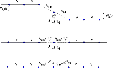
Figure 2: Schematic representation of the model system. The biased system (top) with Hubbard-type interaction on the dot is gauge-equivalent to the system (middle) with time-dependent Peierls phases $\gamma_{L}(t)$ and $\gamma_{R}(t)$ (see Eqs. (39) and (40)). In the local Peierls phase approximation, the Kohn-Sham system (bottom) is assumed to have nonvanishing Peierls phases (Eqs. (44) and (45)) only at the same links as the interaction system (middle).

The TDBCFT presented in Section II.2 guarantees that the bond-currents $J_{mn}$ of the interacting system can be reproduced in a non-interacting KS system with TD Peierls phases $\gamma^{\rm KS}_{mn}(t)$. In the following we make a local approximation for the $\gamma^{\rm KS}_{mn}(t)$: we set them to zero except for those bonds where the external Peierls phases $\gamma_{mn}(t)$ are non-zero, i.e., the bonds connecting the impurity to the leads, see Fig. 2. Within this approximation, we write the only two KS Peierls phases similarly to Eqs. (39-40)

$$\gamma_{\rm L}^{\rm KS}(t)=\int_{0}^{t}{\rm d}t^{\prime}\left(W_{\rm L}(t^{\prime})-v_{\rm KS}(t^{\prime})\right),$$ (44)

and

$$\gamma_{\rm R}^{\rm KS}(t)=\int_{0}^{t}{\rm d}t^{\prime}\left(v_{\rm KS}(t^{\prime})-W_{\rm L}(t^{\prime})\right),$$ (45)

where $\varepsilon_{C}(t)$ is replaced by the on-site KS potential $v_{\rm KS}(t)$ that we write as the sum of the external on-site potential $\varepsilon_{C}(t)$, the Harteee potential $\frac{1}{2}Un(t)$ (with $n(t)$ the TD density at the impurity) and the exchange-correlation (XC) potential $v_{\rm xc}(t)$

$$v_{\rm KS}(t)=\varepsilon_{0}^{\rm C}(t)+\frac{1}{2}Un_{0}(t)+v_{\rm xc}(t)\;.$$ (46)

Note that by a gauge transformation we could go back to the original gauge in which there is an on-site potential instead of the Peierls phases. In the original gauge the KS system is described by the Hamiltonian

$$\hat{H}(t)=\hat{H}_{\rm C}^{\rm KS}(t)+\hat{H}_{\rm L}(t)+\hat{H}_{\rm R}(t)+\hat{H}_{\rm T},$$ (47)

where the lead and the tunneling Hamiltonians, $\hat{H}_{\alpha}(t)$ and $\hat{H}_{T}$, are unchanged compared to the interacting Hamiltonian (i.e., they are given by Eqs. (36) and (37), respectively) and the KS Hamiltonian for the impurity is

$$\hat{H}_{\rm C}^{\rm KS}(t)=\sum_{\sigma}v_{\rm KS}(t)\hat{d}_{\sigma}^{\dagger}\hat{d}_{\sigma}.$$ (48)

We still need to specify the approximation used for the XC potential $v_{\rm xc}(t)$. In this work we use an adiabatic version of the local density approximation (LDA) for the static, non-uniform Hubbard model. The construction of this functional LimaSilvaOliveiraCapelle:03 follows a similar strategy as the one used to construct the usual LDA based on the model of the uniform electron gas. The crucial difference is that the underlying model is the uniform Hubbard model whose exact solution can be constructed via the Bethe ansatz. Just as the XC energy of the uniform electron gas serves as input for the usual LDA, the exact XC energy per site of the uniform Hubbard model then serves as input for the Bethe-ansatz LDA (BALDA) used for non-uniform Hubbard models LimaSilvaOliveiraCapelle:03 ; SilvaLimaMalvezziCapelle:05 . In the context of TDDFT, an adiabatic version of this functional (adiabatic BALDA, ABALDA) local in both space and time, e.g., $v_{\rm xc}[n](i,t)=v_{\rm xc}(n_{i}(t))$, has been suggested by Verdozzi Verdozzi:08 . The form of the BALDA XC potential derives from a parametrization of the XC energy per particle of the uniform Hubbard model. This parametrization deviates somewhat from the exact, numerical XC energy of the Hubbard model XianlongPoliniTosiCampoCapelleRigol:06 ; AkandeSanvito:10 , especially for weak interactions, but here we are not concerned about these differences. The crucial property for our purposes is the existence of a derivative discontinuity at half filling LimaOliveiraCapelle:02 (see discussion below).

The original BALDA has been proposed for a system which not only has the same on-site energy but also the same interaction for all sites and also the hopping connecting neighbouring sites is the same throughout the chain. In Ref. SilvaLimaMalvezziCapelle:05, the BALDA functional has already been used successfully for site-dependent interactions. It should be noted that this is a deviation from the usual LDA philosophy where the XC energy of the uniform gas is used for a non-uniform system but the interaction is unchanged. Here we also take the same approach and use the BALDA for a system with interactions only at one site. In addition, we are interested in situations when the interacting region is weakly connected to two non-interacting leads, i.e., the hopping $V$ within the leads may be different from the coupling $V_{\rm link}$ of the leads to the interacting region. For this situation a generalization of the original BALDA functional has been suggested KurthStefanucciKhosraviVerdozziGross:10 . The explicit form of this modified BALDA XC potential reads

$$v_{\rm xc}[n]=\theta(1-n)v^{(<)}_{\rm xc}[n]-\theta(n-1)v^{(<)}_{\rm xc}[2-n],$$ (49)

where

$$v^{(<)}_{\rm xc}[n]=-\frac{1}{2}{U}n-2V_{\rm link}\left[\cos\left(\frac{\pi n}{2}\right)-\cos\left(\frac{\pi n}{\zeta}\right)\right]\;.$$ (50)

The parameter $\zeta$ is determined by the equation

$$\frac{2\zeta}{\pi}\sin(\pi/\zeta)=4\int_{0}^{\infty}{\rm d}x\,\frac{J_{0}(x)J_{1}(x)}{x[1+\exp({U}x/(2V_{\rm link}))]}$$ (51)

where $J_{i=0,1}(x)$ are Bessel functions. The BALDA XC potential has a discontinuous jump at half-filling LimaOliveiraCapelle:02 :

$$v_{\rm xc}(n=1^{+})-v_{\rm xc}(n=1^{-})=U-4V_{\rm link}\cos\left(\frac{\pi}{\zeta}\right)\;.$$ (52)

Here it is interesting to note that in the limit of very weak coupling ($V_{\rm link}\to 0$) the discontinuity just reduces to $U$ which is the charging energy required to put a second electron on the interacting impurity if it is already occupied by one electron, i.e., in this limit the functional becomes exact. Although the exact XC potential for the Hubbard model is certainly discontinuous, in our situation where a single interacting impurity is coupled to two non-interacting leads, the coupling to the leads introduces some broadening in the levels of the isolated impurity and it is reasonable to expect that this broadening leads to a smoothening of the discontinuity. We therefore introduce a smoothening in our model and use the following XC potential

$$\tilde{v}_{\rm xc}[n]=f(n)v^{(<)}_{\rm xc}[n]-(1-f(n))v^{(<)}_{\rm xc}[2-n],$$ (53)

where

$$f(n)=\frac{1}{\exp((n-1)/a)+1}$$ (54)

and $a$ is a smoothening parameter. In Fig. 3 we show the BALDA XC potential for different values of $U/V_{\rm link}$ using the value $a=10^{-4}$ for the smoothening parameter.

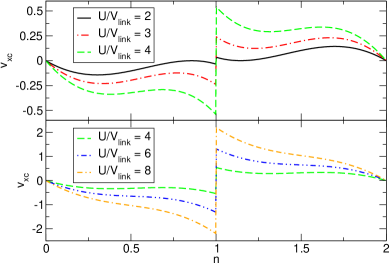
Figure 3: Smoothened BALDA exchange-correlation potential (Eq. (53)) as function of the density for various values of $U/V_{\rm link}$ with smoothing parameter $a=10^{-4}$.

It has recently been shown KurthStefanucciKhosraviVerdozziGross:10 that this discontinuity is crucial to describe Coulomb blockade. Moreover, in a time-dependent picture and in the parameter regime of Coulomb blockade it also prevents the biased system to reach a steady state. More details on these findings will be discussed below.

III.2 Time propagation with embedding

By mapping the interacting problem onto a non-interacting one we have already achieved a considerable simplification. However, we are still dealing with an infinitely extended system which has to be treated numerically. This can be achieved by an embedding technique which maps the infinite system exactly onto a tractable, finite problem.

In the localized site basis the KS Hamiltonian (48) has the matrix structure

$${\bf H}=\left(\begin{array}[]{ccc}{\bf H}_{LL}&{\bf H}_{LC}&0\\ {\bf H}_{CL}&{\bf H}_{CC}&{\bf H}_{CR}\\ 0&{\bf H}_{RC}&{\bf H}_{RR}\\ \end{array}\right).$$ (55)

It is possible to derive the equation of motion for the $k$-th KS single-particle orbital projected onto the central region, $\psi_{k,C}(t)$, which reads

$$\left[i\frac{d}{dt}-{\bf H}_{CC}(t)\right]\psi_{k,C}(t)=\int_{0}^{t}{\rm d}t^{\prime}\;{\bf\Sigma}_{\rm em}(t,t^{\prime})\psi_{k,C}(t^{\prime})$$

$$+\sum_{\alpha}{\bf H}_{C\alpha}{\bf g}_{\alpha\alpha}(t,0)\psi_{k,\alpha}(0),$$ (56)

where

$${\bf\Sigma}_{\rm em}(t,t^{\prime})=\sum_{\alpha=L,R}{\bf H}_{C\alpha}{\bf g}_{\alpha\alpha}(t,t^{\prime}){\bf H}_{\alpha C}$$ (57)

is the retarded embedding self energy. Here, the retarded Green’s function ${\bf g}_{\alpha\alpha}(t,t^{\prime})$ of the isolated lead $\alpha$ satisfies the equation of motion

$$\left[i\frac{d}{dt}-{\bf H}_{\alpha\alpha}(t)\right]{\bf g}_{\alpha\alpha}(t,t^{\prime})=\delta(t-t^{\prime})\;$$ (58)

with boundary conditions ${\bf g}_{\alpha\alpha}(t,t^{+})=0$ and ${\bf g}_{\alpha\alpha}(t,t^{-})=-i$. The TD density at the impurity can be calculated from the KS orbitals as in Eq. (2), i.e.,

$$n(t)=\sum_{k}^{\rm occ}|\psi_{k,C}(t)|^{2}\;,$$ (59)

where the sum runs over the occupied KS states. In the present work we use the algorithm described in Ref. KurthStefanucciAlmbladhRubioGross:05, to propagate Eq. (56) starting from the self-consistent BALDA ground state of the coupled lead-dot-lead system.

IV The derivative discontinuity and its connection to Coulomb blockade

IV.1 Ground state and non-equilibrium steady state

We will use the KS Hamiltonian in the BALDA approximation to describe transport for our model of a single interacting impurity connected to two non-interacting tight-binding leads. This model has been studied extensively in the literature, and the results from other methods can be used for a validation of our KS treatment. In the present Section we first assess the quality of our approximate BALDA functional in the ground state by comparing to recent Quantum Monte Carlo (QMC) results for the same model system. Then we look into the nonequilibrium steady state for the system exposed to a DC bias in the leads, assuming that such a steady state exists.

Using the techniques of non-equilibrium Green’s functions one can derive a self-consistency condition for the ground or steady-state electron density $n^{\infty}$ at the impurity which reads

$$n^{\infty}=2\sum_{\alpha={\rm L,R}}\int_{-\infty}^{\varepsilon_{F}+W_{\alpha}}\frac{{\rm d}\omega}{2\pi}\Gamma(\omega-W_{\alpha})|G(\omega)|^{2}\;.$$ (60)

Here, $W_{\alpha}$ ($\alpha={\rm L,R}$) is the constant bias applied in lead $\alpha$ (of course, the ground state density is obtained for $W_{\rm L}=W_{\rm R}=0$) and

$$G(\omega)=\left(\omega-v_{\rm KS}[n^{\infty}]-\sum_{\alpha={\rm L,R}}\Sigma_{\alpha}(\omega-W_{\alpha})\right)^{-1}$$ (61)

is the retarded Green’s function in frequency space at the impurity. $\Sigma_{\alpha}(\omega)$ is the Fourier transform of the $\alpha$-lead contribution to the embedding self energy (57) which, for the present case of non-interacting tight-binding leads with vanishing onsite energies, $\varepsilon_{\alpha}=0$, is given explicitly by

$$\Sigma_{\alpha}(\omega)=\Lambda_{\alpha}(\omega)-\frac{i}{2}\Gamma_{\alpha}(\omega)$$ (65)

$$= \frac{V_{\rm link}^{2}}{2V_{\alpha}^{2}}\left\{\begin{array}[]{ll}\omega_{\alpha}-\sqrt{\omega_{\alpha}^{2}-4V_{\alpha}^{2}}&\mbox{\hskip 11.38109ptfor $\omega_{\alpha}>2V_{\alpha}$}\\ \omega_{\alpha}+\sqrt{\omega_{\alpha}^{2}-4V_{\alpha}^{2}}&\mbox{\hskip 11.38109ptfor $\omega_{\alpha}<-2V_{\alpha}$}\\ \omega_{\alpha}-i\sqrt{4V_{\alpha}^{2}-\omega_{\alpha}^{2}}&\mbox{\hskip 11.38109ptfor $|\omega_{\alpha}|\leq 2V_{\alpha}$}\end{array}\right.\;\;\;$$

with real and imaginary parts $\Lambda_{\alpha}(\omega)$ and $\Gamma_{\alpha}(\omega)$, respectively. Finally, the total width function is $\Gamma(\omega)=\sum_{\alpha}\Gamma_{\alpha}(\omega)$ and $\varepsilon_{F}$ is the Fermi energy of the contacted system in the ground state.

We have first solved Eq. (60) for the ground state density $n_{0}:=n^{\infty}$ for $W_{\rm L}=W_{\rm R}=0$ and compared to recent QMC calculations presented by Wang et al. in Ref. WangSpataruHybertsenMillis:08, . Here we focus on the dependence of $n_{0}$ on the on-site energy $\varepsilon_{C}$ at the impurity. We set $\varepsilon_{F}=0$ (half filling of the leads) and for the Hubbard interaction we use $U=0.105,0.21,0.42,0.84$ (all energies are given in units of the equal hopping in left and right leads $V_{\rm L}=V_{\rm R}=V$). For the hopping between leads and impurity we take a weak $V_{\rm link}=0.1803$. In order to achieve a meaningful comparison to the QMC data, the value of our $V_{\rm link}$ is a factor of $1/\sqrt{2}$ smaller than the one used in Ref. WangSpataruHybertsenMillis:08, since Wang et al. considered an impurity coupled to a single lead only verdozzi_comm . For the smoothening parameter we choose the value $a=10^{-4}$. Fig. 4 shows the ground state density as function of on-site energy $\varepsilon_{C}$. We see that the QMC and BALDA results agree surprisingly well, especially for weak interactions. For strong interactions the BALDA develops a clear Coulomb blockade step, i.e., the density hardly changes over a significant range of onsite energies. Although the step in BALDA extends over a smaller range of onsite energies than in QMC, the agreement is still quite reasonable. Already at this stage it is clear that the feature which gives rise to the Coulomb blockade step is the derivative discontinuity built into the BALDA functional.

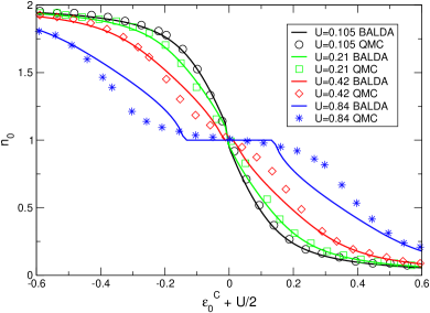
Figure 4: Comparison of BALDA and Quantum Monte Carlo (QMC) ground state densities at the impurity as function of onsite energy $\varepsilon_{0}^{C}$ for different values of the interaction. The coupling between leads and impurity is $V_{\rm link}=0.1803$. All energies are given in units of the hopping $V$ in the leads. The QMC results were extracted from Ref. WangSpataruHybertsenMillis:08, .

Now we turn our attention to the biased, non-equilibrium situation. If we assume that the system evolves toward a steady state in the long time limit then the steady-state value of the density at the impurity is given by the self-consistent solution of Eq. (60). We solve the latter for different values of the bias $W_{\rm L}$ applied in the left lead. The system parameters are $\varepsilon_{C}=2$, $U=2$, $\varepsilon_{F}=1.5$ and $a=10^{-4}$.

In the left panel of Fig. 5 we show the steady state density as function of the applied bias for different values of the hopping $V_{\rm link}$ between leads and impurity. We clearly see a plateau in the steady-state density at unity, i.e., when the impurity is occupied by exactly one electron. This plateau becomes wider and more step-like as $V_{\rm link}$ decreases which corresponds to the usual picture of Coulomb blockade: the dot can only be occupied by zero, one, or two electrons, and the energy cost for double occupancy is given by the Hubbard interaction $U$. It is important to emphasize here that in the plateau region it is crucial that we used an XC potential with a smoothened discontinuity. If one uses the truly discontinuous XC potential, the steady-state condition actually does not have any solution at all in this parameter region, indicating that the initial steady-state assumption was not justified. This point will be further investigated in the next Section.

In the right panel of Fig. 5 we show the steady-state densities for the same parameter range if one uses the Hartree approximation, i.e., when $v_{\rm xc}$ in Eq. (46) is set to zero. One clearly sees that in this case the step in the steady-state density is completely absent. Instead, for small $V_{\rm link}$ the steady-state density rises almost linearly within a certain bias range. For larger values of $V_{\rm link}$, the Hartree and BALDA steady-state densities are qualitatively quite similar.

Figure 5: Steady state density as function of the applied bias $W_{L}$ for different values of $V_{\rm link}$. Left panel: BALDA steady state densities, right panel: Hartree steady state densities.

IV.2 Time-dependent transport

In the previous Section we assumed that under application of a DC bias the system evolves towards a steady state for which we then solved a self-consistency condition to obtain the steady-state density. In the present Section we will show that for certain parameters the steady-state assumption is actually not always justified: when perturbing the system, which is initially in its ground state, by switching on a DC bias the time evolution does not necessarily lead to a steady state but rather to an oscillatory state of dynamical density oscillations.

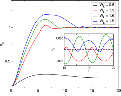
Figure 6: TD density in BALDA for different values of the bias $W_{L}$ for $V_{\rm link}=0.3$. Inset: Magnification of the TD density at large times. The straight line at unity is a guide for the eye.

In Fig. 6 we show the time evolution of the quantum-dot density from its intial, ground-state value when, at $t=0$, a DC bias is suddenly switched on in the left lead, i.e., $W_{\rm L}(t)=\theta(t)W_{\rm L}$ with $W_{\rm L}=0.5,1.3,1.6,1.9$. The parameters are the same as those used for Fig. 5 with $V_{\rm link}=0.3$. According to the steady-state picture of Fig. 5, the first value $W_{L}=0.5$ corresponds to the rising flank of the density as function of bias while the other biases correspond to the plateau. The TD density corresponding to bias $W_{\rm L}=0.5$ can be seen to evolve smoothly towards its steady state value. However, looking closely at the evolution of the density for the other bias values (inset of Fig. 6) one can see that for these cases the system does not evolve towards a steady state but rather approaches a dynamical state of periodically oscillating density. Furthermore, the density oscillates around unity, i.e., single occupancy of the impurity. The amplitude of these oscillations is rather small, of the order of $5\times 10^{-3}$. We also note that the larger the value of the bias (in the range of the plateau of Fig. 5), the larger the fraction of time for which the density exceeds the critical value of unity.

The qualitative difference of the response of the system for biases within and outside the step region of Fig. 5 becomes quite apparent when looking at the time-dependent KS potentials (left panels of Fig. 7) and currents through the impurity (right panels of the same figure). While for the bias outside the step region ($W_{\rm L}=0.5$) both quantities behave smoothly, for the other biases the KS potentials show rapid variations which are due to the discontinuity at $n=1$: as long as the time-dependent density stays below or above unity, the KS potential changes smoothly in time. However, when the density crosses unity, the KS potential jumps discontinuously (or very rapidly for the smoothened KS potentials used here). The rapid variation of the KS potential allows us to understand why for these cases a steady state is not achieved: consider the situation when the time-dependent density crosses the critical value of unity from below. At the instant $t_{c1}$ when the jump in the KS potential occurs, the rate of change of the density is positive, $\dot{n}(t_{c1})>0$, and immediately after $t_{c1}$ the density continues to grow because the maximum rate of change of the density is limited by the inertia of the electrons. However, for times right after $t_{c1}$ the significant increase of the KS potential tends to push down the density, i.e., $\ddot{n}(t)<0$, and therefore $n(t)$ will cross the critical value of unity from above at some time $t_{c2}>t_{c1}$. At that time $\dot{n}(t_{c2})<0$, the KS potential will suddenly be lowered and electrons will be attracted by the quantum dot, i.e., $\ddot{n}(t)>0$. Therefore, the density will eventually crosses unity at some time $t_{c3}>t_{c2}$ from below and the cycle will start over.

The above results have been obtained with an XC potential with a smoothened discontinuity for which, in principle, the condition for the steady-state density discussed in the previous Section does have a solution. This solution is not reached by the time propagation because the rate of change of the density is limited by $V_{\rm link}$ Verdozzi:08 . The rate of change of the KS potential when the density crosses the (smoothened) discontinuity is instead limited by the smoothening parameter $a^{-1}$. Therefore the steady state should not be attained whenever the rate of change of the KS potential is larger than the largest possible rate of change of the density.

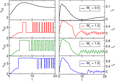
Figure 7: Time-dependent KS potentials and currents at the impurity for different values of the bias $W_{L}$ for $V_{\rm link}=0.3$. Left panels: BALDA KS potentials, right panels: TD currents at the impurity site.

The time-dependent currents in the Coulomb blockade regime (lower three right panels of Fig. 7) show sawtooth-like oscillations at the impurity site. By the equation of motion for the currents, this is consistent with the fact that the KS potentials form a train of almost rectangular potential steps. In contrast, the current away from the Coulomb blockade regime (upper right panel of Fig. 7) evolves smoothly towards its steady state value. This is qualitatively similar to the behaviour which is found for time-dependent Hartree calculations (in any parameter regime). Finally, we would like to point out that the oscillations just described are entirely due to electron correlations and are therefore different from oscillations occuring due to the presence of single-particle bound states Stefanucci:07 ; KhosraviKurthStefanucciGross:08 ; KhosraviStefanucciKurthGross:09 .

V Conclusions

In the present work we have described the difficulties in generalizing the fundamental Runge-Gross proof of time-dependent density functional theory to systems described by a lattice Hamiltonian. To overcome these difficulties we have employed the time-dependent bond current instead of the density as basic variable. We were then able to prove a one-to-one correspondence between time-dependent bond currents and Peierls phases describing the electromagnetic field on the lattice and therefore proposed a time-dependent bond current functional theory as the proper extension of TDDFT to lattice systems.

In a second part we have described a time-dependent approach to electron transport in model systems using this TDBCFT. We proposed a local Peierls phase approximation assuming that the Peierls phases of the noninteracting KS system are nonvanishing only for the same links as for the interacting case. A simple model of an interacting impurity connected to two noninteracting leads has been studied employing a functional which exhibits an explicit derivative discontinuity leading to a time-dependent KS potential which jumps discontinuously as the particle number on the impurity crosses an integer LeinKuemmel:05 . It has been demonstrated that this discontinuity is (i) crucial to describe Coulomb blockade and (ii) prevents the system from reaching a steady state by time-evolution out of the initial ground state upon application of a bias in the leads. Instead we find that after some transient time the system reaches a dynamical state of undamped density oscillations. In this picture, Coulomb blockade manifests itself as a dynamic phenomenon of sequentially charging and discharging the impurity.

Here we demonstrated the crucial role played by the discontinuity in the XC potential to properly describe Coulomb blockade, a physical phenomenon which is due to electronic correlations, for a simple model system. This model is not easily generalized to more complicated situations such as, e.g., more orbitals or degrees of freedom per site or more complicated lattices. As for the latter case, there have recently been activities to construct the XC energy per particle which also display a derivative discontinuity for more complicated model systems such as a graphene-like hexagonal Hubbard lattice IjaesHarju:10 or the Hubbard model in three dimensions KarlssonPriviteraVerdozzi . However, the challenge remains to construct practical and universal approximations with a derivative discontinuity not only for lattice systems but also for systems described by continuum Hamiltonians.

- (1) G. Stefanucci and C.-O. Almbladh, Phys. Rev. B 69, 195318 (2004); Europhys. Lett. 67, 14 (2004).
- (2) S. Kurth, G. Stefanucci, C.-O. Almbladh, A. Rubio, and E.K.U. Gross, Phys. Rev. B 72, 035308 (2005).
- (3) E. Runge and E.K.U. Gross, Phys. Rev. Lett. 52, 997 (1984).
- (4) R. van Leeuwen, Phys. Rev. Lett. 82, 3863 (1999).
- (5) M. Ruggenthaler and R. van Leeuwen, arXiv:1011.3375 (2010).
- (6) P. Hohenberg and W. Kohn, Phys. Rev. 136, B864 (1964).
- (7) W. Kohn and L.J. Sham, Phys. Rev. 140, A1133 (1965).
- (8) R. Baer, J. Chem. Phys. 128, 044103 (2008).
- (9) Y. Li and C.A. Ullrich, J. Chem. Phys. 129, 044105 (2008).
- (10) C. Verdozzi, Phys. Rev. Lett. 101, 166401 (2008).
- (11) J.P. Perdew, R.G. Parr, M. Levy, and J.L. Balduz, Phys. Rev. Lett. 49, 1691 (1982).
- (12) S. Kurth, G. Stefanucci, E. Khosravi, C. Verdozzi, and E.K.U. Gross, Phys. Rev. Lett. 104, 236801 (2010).
- (13) G. Stefanucci, E. Perfetto, and M. Cini, Phys. Rev. B 81, 115446 (2010).
- (14) G. Vignale, Phys. Rev. B 70, 201102(R) (2004).
- (15) For the case of TD current DFT for continuum Hamiltonians, the convergence issue for physical systems has been discussed in Ref. Vignale:04, .
- (16) I. Tokatly, arXiv:1011.2715 (2010).
- (17) K. Burke, R. Car, and R. Gebauer, Phys. Rev. Lett. 94, 146803 (2005).
- (18) P. Bokes, F. Corsetti, and R.W. Godby, Phys. Rev. Lett. 101, 046402 (2008).
- (19) Z. Zhou and S.-I. Chu, Europhys. Lett. 88, 17008 (2009).
- (20) X. Zheng G.-H. Chen, Y. Mo, S.-K. Koo, H. Tian, C.-Y. Yam, and Y.-J. Yan, J. Chem. Phys. 133, 114101 (2010).
- (21) V. Moldoveanu, A. Manolescu, C.-S. Tang, and V. Gudmundsson, Phys. Rev. B 81, 155442 (2010).
- (22) P. Myöhänen, A. Stan, G. Stefanucci, and R. van Leeuwen, Europhys. Lett. 84, 67001 (2008).
- (23) P. Myöhänen, A. Stan, G. Stefanucci, and R. van Leeuwen, Phys. Rev. B 80, 115107 (2009).
- (24) M.P. von Friesen, C. Verdozzi, and C.-O. Almbladh, Phys. Rev. B 82, 155108 (2010).
- (25) F. Heidrich-Meisner, A. E. Feiguin, and E. Dagotto, Phys. Rev. B 79, 235336 (2009).
- (26) F. Heidrich-Meisner, I. González, K.A. Al-Hassanieh, A.E. Feiguin, M.J. Rozenberg, and E. Dagotto, Phys. Rev. B 82, 205110 (2010).
- (27) A. Branschädel, G. Schneider, P. Schmitteckert, Ann. Phys. (Berlin) 522, 657 (2010).
- (28) X. Oriols, Phys. Rev. Lett. 98, 066803 (2007).
- (29) L. Mühlbacher and E. Rabani, Phys. Rev. Lett. 100, 176403 (2008).
- (30) P. Werner, T. Oka, M. Eckstein, and A.J. Millis, Phys. Rev. B 81, 035108 (2010).
- (31) P.W. Anderson, Phys. Rev. 124, 41 (1961).
- (32) N.A. Lima, M.F. Silva, L.N. Oliveira, and K. Capelle, Phys. Rev. Lett. 90, 146402 (2003).
- (33) M.F. Silva, N.A. Lima, A.L. Malvezzi, and K. Capelle, Phys. Rev. B 71, 125130 (2005).
- (34) G. Xianlong, M. Polini, M.P. Tosi, V.L. Campo, K. Capelle, and M. Rigol, Phys. Rev. B 73, 165120 (2006).
- (35) A. Akande and S. Sanvito, Phys. Rev. B 82, 245114 (2010).
- (36) N.A. Lima, L.N. Oliveira, and K. Capelle, Europhys. Lett. 60, 601 (2002).
- (37) X. Wang, C. D. Spataru, M. S. Hybertsen, and A. J. Millis, Phys. Rev. B 77, 045119 (2008).
- (38) C. Verdozzi, private communication.
- (39) G. Stefanucci, Phys. Rev. B 75, 195115 (2007).
- (40) E. Khosravi, S. Kurth, G. Stefanucci, and E.K.U. Gross, Appl. Phys. A 93, 355 (2008).
- (41) E. Khosravi, G. Stefanucci, S. Kurth, and E.K.U. Gross, Phys. Chem. Chem. Phys. 11, 4535 (2009).
- (42) M. Lein, S. Kümmel, Phys. Rev. Lett. 94, 143003 (2005).
- (43) M. Ijäs, A. Harju, Phys. Rev. B 82, 235111 (2010).
- (44) D. Karlsson, A. Privitera, and C. Verdozzi, arXiv:1004.2264 (2010).