The Planar Slope Number of Planar Partial 3-Trees of Bounded Degree

Abstract

It is known that every planar graph has a planar embedding where edges are represented by non-crossing straight-line segments. We study the planar slope number, i.e., the minimum number of distinct edge-slopes in such a drawing of a planar graph with maximum degree $\Delta$. We show that the planar slope number of every planar partial 3-tree and also every plane partial 3-tree is at most ${\cal O}(\Delta^{5})$. In particular, we answer the question of Dujmović et al. [Computational Geometry 38 (3), pp. 194–212 (2007)] whether there is a function $f$ such that plane maximal outerplanar graphs can be drawn using at most $f(\Delta)$ slopes.
Keywords: graph drawing; planar graphs; slopes; planar slope number

1 Introduction

The slope number of a graph $G$ was introduced by Wade and Chu [12]. It is defined as the minimum number of distinct edge-slopes in a straight-line drawing of $G$. Clearly, the slope number of $G$ is at most the number of edges of $G$, and it is at least half of the maximum degree $\Delta$ of $G$.

Dujmović et al. [2] asked whether there was a function $f$ such that each graph with maximum degree $\Delta$ could be drawn using at most $f(\Delta)$ slopes. In general, the answer is no due to a result of Barát et al. [1]. Later, Pach and Pálvölgyi [11] and Dujmović et al. [3] proved that for every $\Delta\geq 5$, there are graphs of maximum degree $\Delta$ that need an arbitrarily large number of slopes.

On the other hand, Keszegh et al. [7] proved that every graph of maximum degree three can be drawn using at most five slopes, and if we additionally assume that the graph is connected and has at least one vertex of degree less than three then four slopes suffice. Mukkamala and Szegedy [10] have shown that four slopes also suffice for every connected cubic graph. Dujmović et al. [3] give a number of bounds in terms of the maximum degree: for interval graphs, cocomparability graphs, or AT-free graphs. All the results mentioned so far are related to straight-line drawings which are not necessarily non-crossing.

It is known that every planar graph $G$ can be drawn so that edges of $G$ are represented by non-crossing segments [6]. We call such a planar drawing a straight-line embedding of $G$. In this paper, we examine the minimum number of slopes in a straight-line embedding of a planar graph.

In this paper, we make the (standard) distinction between planar graphs, which are graphs that admit a plane embedding, and plane graphs, which are graphs accompanied with a fixed prescribed combinatorial embedding, i.e., a prescribed face structure, including a prescribed outer face. Accordingly, we distinguish between the planar slope number of a planar graph $G$, which is the smallest number of slopes needed to construct any straight-line embedding of $G$, as opposed to the plane slope number of a plane graph $G$, which is the smallest number of slopes needed to realize the prescribed combinatorial embedding of $G$ as a straight-line embedding.

The research of slope parameters related to plane embedding was initiated by Dujmović et al. [2]. In [4], there are numerous results for the plane slope number of various classes of graphs. For instance, it is proved that every plane $3$-tree can be drawn using at most $2n$ slopes, where $n$ is its number of vertices. It is also shown that every $3$-connected plane cubic graph can be drawn using three slopes, except for the three edges on the outer face.

Recently, Keszegh, Pach and Pálvölgyi [8] have shown that any planar graph of maximum degree $\Delta$ can be drawn with $2^{{\cal O}(\Delta)}$ slopes. Their argument is based on a representation of planar graph by touching disks.

In this paper, we study both the plane slope number and the planar slope number. The lower bounds of [1, 3, 11] for bounded-degree graphs do not apply to our case, because the constructed graphs with large slope numbers are not planar. Moreover, the upper bounds of [7, 10] give drawings that contain crossings even for planar graphs.

For a fixed $k\in\mathbb{N}$, a $k$-tree is defined recursively as follows. A complete graph on $k$ vertices is a $k$-tree. If $G$ is a $k$-tree and $K$ is a $k$-clique of $G$, then the graph formed by adding a new vertex to $G$ and making it adjacent to all vertices of $K$ is also a $k$-tree. A subgraph of a $k$-tree is called a partial $k$-tree.

We present several upper bounds on the plane and planar slope number in terms of the maximum degree $\Delta$. The most general result of this paper is the following theorem, which deals with plane partial 3-trees.

Theorem 1.1.

The plane slope number of any plane partial 3-tree with maximum degree $\Delta$ is at most ${\cal O}(\Delta^{5})$.

Note that the above theorem implies that the planar slope number of any planar partial 3-tree is also at most ${\cal O}(\Delta^{5})$.

Since every outerplanar graph is also a partial 3-tree, the result above answers a question of Dujmović et al. [4], who asked whether a plane maximal outerplanar graph can be drawn using at most $f(\Delta)$ slopes.

Unlike the results of Keszegh, Pach and Pálvölgyi [8], our arguments are only applicable to a restricted class of planar graphs. On the other hand, our bound is polynomial in $\Delta$ rather than exponential, and moreover, our proof is constructive.

In the special case of series-parallel graphs of maximum degree at most 3, we are able to prove a better (in fact optimal) upper bound.

Theorem 1.2.

Any series-parallel graph with maximum degree at most 3 has planar slope number at most 3.

Extended abstract of this paper was presented at Graph Drawing 2009 [5]. Note that in that version Theorem 1.1 was stated with bound ${\cal O}(2^{{\cal O}(\Delta)})$.

2 Preliminaries

Let us introduce some basic terminology and notation that will be used throughout this paper.

Let $s$ be a segment in the plane. The smallest angle $\alpha\in[0,\pi)$ such that $s$ can be made horizontal by a clockwise rotation by $\alpha$, is called the slope of $s$. The directed slope of a directed segment is an angle $\alpha^{\prime}\in[0,2\pi)$ defined analogously.

A plane graph is called a near triangulation if all its faces, except possibly the outer face, are triangles.

3 Plane partial 3-trees

In this section we present the proof of Theorem 1.1. We start with some observations about the structure of plane 3-trees. Throughout this section, we assume that $\Delta$ is a fixed integer.

It is known that any plane 3-tree can be generated from a triangle by a sequence of vertex-insertions into inner faces. Here, a vertex-insertion is an operation that consists of creating a new vertex in the interior of a face, and then connecting the new vertex to all the three vertices of the surrounding face, thus subdividing the face into three new faces.

For a plane partial 3-tree $G$ we define the level of a vertex $v$ as the smallest integer $k$ such there is a set $V_{0}$ of $k$ vertices of $G$ with the property that $v$ is on the outer face of the plane graph $G-V_{0}$. Let $G$ be a plane partial 3-tree. An edge of $G$ is called balanced if it connects two vertices of the same level of $G$. An edge that is not balanced is called tilted. Similarly, a face of $G$ whose all vertices belong to the same level is called balanced, and any other face is called tilted. In a plane 3-tree, the level of a vertex $v$ can also be equivalently defined as the length of the shortest path from $v$ to a vertex on the outer face. However, this definition cannot be used for plane partial 3-trees.

Note that whenever we insert a new vertex $v$ into an inner face of a 3-tree, the level of $v$ is one higher than the minimum level of its three neighbors; note also that the level of all the remaining vertices of the 3-tree is not affected by the insertion of a new vertex.

Let $u,v$ be a pair of vertices forming an edge. A bubble over $uv$ is an outerplanar plane near triangulation that contains the edge $uv$ on the boundary of the outer face. The edge $uv$ is called the root of the bubble. A trivial bubble is a bubble that has no other edge apart from the root edge. A double bubble over $uv$ is a union of two bubbles over $uv$ which have only $u$ and $v$ in common and are attached to $uv$ from its opposite sides. A leg is a graph $L$ created from a path $P$ by adding a double bubble over every edge of $P$. The path $P$ is called the spine of $L$ and the endpoints of $P$ are also referred to as the endpoints of the leg. Note that a single vertex is also considered to form a leg.

A tripod is a union of three legs which share a common endpoint. A spine of a tripod is the union of the spines of its legs. Observe that a tripod is an outerplanar graph. The vertex that is shared by all the three legs of a tripod is called the central vertex.

Let $G$ be a near triangulation, let $\Phi$ be an inner face of $G$. Let $T$ be a tripod with three legs $X,Y,Z$ and a central vertex $c$. An insertion of tripod $T$ into the face $\Phi$ is the operation performed as follows. First, insert the central vertex $c$ into the interior of $\Phi$ an connect it by edges to the three vertices of $\Phi$. This subdivides $\Phi$ into three subfaces. Extend $c$ into an embedding of the whole tripod $T$, by embedding a single leg of the tripod into the interior of each of the three subfaces. Next, connect every non-central vertex of the spine of the tripod to the two vertices of $\Phi$ that share a face with the corresponding leg. Finally, connect each non-spine vertex $v$ of the tripod to the single vertex of $\Phi$ that shares a face with $v$. See Figure 1. Observe that the graph obtained by a tripod insertion into $\Phi$ is again a near triangulation.

Figure 1: An example of a tripod consisting of vertices of level 1 in a plane 3-tree.

Lemma 3.1.

Let $G$ be a graph. The following statements are equivalent:

1. $G$ is a plane 3-tree, i.e., $G$ can be created from a triangle by a sequence of vertex insertions into inner faces.

2. $G$ can be created from a triangle by a sequence of tripod insertions into inner faces.

3. $G$ can be created from a triangle by a sequence of tripod insertions into balanced inner faces.

Proof.

Clearly, (3) implies (2).

To observe that (2) implies (1), it suffices to notice that a tripod insertion into a face $\Phi$ can be simulated by a sequence of vertex insertions: first insert the central vertex of a tripod into $\Phi$, then insert the vertices of the spine into the resulting subfaces, and then create each bubble by inserting vertices into the face that contains the root of the bubble and its subsequent subfaces.

To show that (1) implies (3), proceed by induction on the number of levels in $G$. If $G$ only has vertices of level $0$, then it consists of a single triangle and there is nothing to prove. Assume now that the $G$ is a graph that contains vertices of $k>0$ distinct levels, and assume that any 3-tree with fewer levels can be generated by a sequence of balanced tripod insertions by induction.

We will show that the vertices of level $k$ induce in $G$ a subgraph whose every connected component is a tripod, and that each of these tripod is inserted inside a triangle whose vertices have level $k-1$.

Let $C$ be a connected component of the subgraph induced in $G$ by the vertices of level $k$. Let $v_{1},v_{2},\dotsc,v_{m}$ be the vertices of $C$, in the order in which they were inserted when $G$ was created by a sequence of vertex insertions. Let $\Phi$ be the triangle into which the vertex $v_{1}$ was inserted, and let $x,y$ and $z$ be the vertices of $\Phi$. Necessarily, all three of these vertices have level $k-1$. Each of the vertices $v_{2},\dotsc,v_{m}$ must have been inserted into the interior of $\Phi$, and each of them must have been inserted into a face that contained at least one of the three vertices of $\Phi$.

Note that at each point after the insertion of $v_{1}$, there are exactly three faces inside $\Phi$ that contain a pair of vertices of $\Phi$; each of these three faces is incident to an edge of $\Phi$. Whenever a vertex $v_{i}$ is inserted into such a face, the subgraph induced by vertices of level $k$ grows by a single edge. These edges form a union of three paths that share the vertex $v_{1}$ as their common endpoint.

On the other hand, when a vertex $v_{i}$ is inserted into a face formed by a single vertex of $\Phi$ and a pair of previously inserted vertices $v_{j}$, $v_{\ell}$, then the graph induced by vertices of level $k$ grows by two new edges $v_{i}v_{j}$ and $v_{i}v_{\ell}$, as well as a new triangular face with vertices $v_{i},v_{j},v_{\ell}$.

With these observations, it is easily checked (e.g., by induction on $i$) that for every $i\geq 1$, the subgraph of $G$ induced by the vertices $v_{1},\dotsc,v_{i}$ is a tripod inserted into $\Phi$. From this fact, it follows that the whole graph $G$ may have been created by a sequence of tripod insertions into balanced faces. ∎

Note that when we insert a tripod into a balanced face, all the vertices of the tripod will have the same level (which will be one higher than the level of the face into which we insert the tripod). In particular, each balanced face we create by this insertion is an inner face of the inserted tripod.

Recall that a plane partial 3-tree is a plane graph that is a subgraph of a 3-tree. Kratochvíl and Vaner [9] have shown that every plane partial 3-tree $G$ is in fact a subgraph of a plane 3-tree. Furthermore, if a plane partial 3-tree $G$ has at least three vertices, it is in fact a spanning subgraph of a plane 3-tree, i.e., it can be extended into a plane 3-tree by only adding edges.

Unfortunately, the plane 3-tree that contains a plane partial 3-tree $G$ may in general require arbitrarily large vertex-degrees, even if the maximum degree of $G$ is bounded. Thus, the result of Kratochvíl and Vaner does not allow us to directly simplify the problem to plane 3-trees drawing.

To overcome this difficulty, we introduce the notion of ‘plane semi-partial 3-tree’, which can be seen as an intermediate concept between plane 3-trees and plane partial 3-trees.

Definition 3.2.

A graph $G$ is called a plane semi-partial 3-tree if $G$ is obtained from a plane 3-tree $H$ by erasing some of the tilted edges of $H$.

Our goal is to prove that every plane partial 3-tree of maximum degree $\Delta$ can be drawn with at most ${\cal O}(\Delta^{5})$ slopes. We obtain this result as a direct consequence of two main propositions, stated below.

Proposition 3.3.

Any connected plane partial 3-tree of maximum degree $\Delta$ is a subgraph of a plane semi-partial 3-tree of maximum degree at most $37\Delta$.

Proposition 3.4.

For every $\Delta$ there is a set $S$ of at most ${\cal O}(\Delta^{5})$ slopes with the property that any plane semi-partial 3-tree of maximum degree $\Delta$ has a straight-line embedding whose edge-slopes all belong to $S$.

We begin by proving Proposition 3.3.

3.1 Proof of Proposition 3.3

We begin by a simple lemma, which shows that the deletion of tilted edges from a plane 3-tree does not affect the level of vertices.

Lemma 3.5.

Let $H=(V,E)$ be a plane 3-tree, let $T$ be a set of tilted edges of $H$, let $G=(V,E\setminus T)$ be a semi-partial 3-tree. Let $v$ be a vertex of level $k$ with respect to $H$. Then $v$ has level $k$ in $G$ as well.

Proof.

Fix a vertex $v$ of level $k$ in $H$. Of course, the deletion of an edge may only decrease the level of a vertex, so $v$ has level at most $k$ in $G$. On the other hand, it follows from Lemma 3.1 that every vertex of level $k$ in $H$ is separated from the outer face by $k$ nested triangles $C_{0},C_{1},\dotsc C_{k-1}$, where $C_{i}$ is a triangle formed by balanced edges that belong to level $i$. Since every balanced edge of $H$ belongs to $G$ as well, we know that all the triangles $C_{0},C_{1},\dotsc C_{k-1}$ belong to $G$, showing that $v$ has level at least $k$. It follows that the level of $v$ is preserved by the deletion of tilted edges. ∎

Let $G=(V,E)$ be a plane semi-partial 3-tree obtained from a plane 3-tree $H=(V,E^{\prime})$ by the deletion of several tilted edges. As a consequence of the previous lemma, we see that an edge $e\in E$ is tilted in $G$ if and only if it is tilted in $H$.

Assume now that $F$ is a connected plane partial 3-tree with maximum degree $\Delta\geq 1$ and at least three vertices. Our goal is to show that there is a plane semi-partial 3-tree $G$ with maximum degree at most $37\Delta$ that contains $F$ as a spanning subgraph. The following definition introduces the key notion of our proof.

Definition 3.6.

Let $F$ be a connected plane partial 3-tree with maximum degree $\Delta$, and let $k$ be an integer. We say that a 3-tree $H$ correctly covers $F$ up to level $k$, if the following conditions are satisfied:

• $F$ is a spanning subgraph of $H$.

• Let $V^{\leq k}$ denote the set of vertices that have level at most $k$ in $H$. For every vertex $v\in V^{\leq k}$ there are at most $36\Delta$ balanced edges of $H$ that are incident to $v$.

Furthermore, we say that $H$ correctly covers $F$ at all levels if, for any $k$, $H$ correctly covers $F$ up to level $k$.

As mentioned before, Kratochvíl and Vaner [9] have shown that every plane partial 3-tree $F$ is a spanning subgraph of a plane 3-tree $H$. Note that such a 3-tree $H$ correctly covers $F$ up to level 0, because every vertex at level 0 is adjacent to two balanced edges.

Our proof of Proposition 3.3 is based on the following lemma.

Lemma 3.7.

For every connected partial 3-tree $F$ there is a 3-tree $H$ that correctly covers $F$ at all levels.

Before we prove the lemma, let us show how it implies Proposition 3.3.

Proof of Proposition 3.3 from Lemma 3.7.

Let $F$ be a plane partial 3-tree of maximum degree $\Delta$, and let $H$ be the 3-tree that correctly covers $F$ at all levels. Define a semi-partial 3-tree $G$ which is obtained from $H$ by erasing all the tilted edges of $H$ that do not belong to $F$. By construction, $G$ is a semi-partial 3-tree that contains $F$ as a subgraph. Moreover, every vertex of $G$ is adjacent to at most $\Delta$ tilted edges and at most $36\Delta$ balanced edges, so $G$ has maximum degree at most $37\Delta$. ∎

Let us now turn to the proof of Lemma 3.7.

Proof.

Let $F$ be a partial 3-tree with maximum degree $\Delta$, and assume for contradiction that there is no graph $H$ that would correctly cover $F$. Let $k$ be the largest integer such that there is a graph $H$ that correctly covers $F$ up to level $k$. We have seen that $k\geq 0$. On the other hand, we clearly have $k<|V(F)|$. Thus, $k$ is well defined.

Fix a graph $H$ correctly covering $F$ up to level $k$. By our assumption, $H$ has vertices of level greater than $k$. We will now define a 3-tree $H^{\prime}$ that correctly covers $F$ up to level $k+1$, which contradicts the maximality of $k$.

Note that it is sufficient to ensure that $H^{\prime}$ is constructed by a sequence of balanced tripod insertions in which all the tripods inserted at level at most $k+1$ have degrees bounded by $36\Delta$.

We construct $H^{\prime}$ in such a way that it coincides with $H$ on vertices of level at most $k$; more precisely, if $u$ and $v$ are two vertices of level at most $k$ in $H$, then $u$ and $v$ are connected by an edge of $H^{\prime}$ if and only if they are connected by an edge of $H$. Notice that this property guarantees that the vertices at level at most $k$ in $H$ are at the same level in $H^{\prime}$ as in $H$. Let $H^{\leq k}$ be the subgraph of $H$ induced by the vertices of level at most $k$. $H^{\leq k}$ is a 3-tree.

Let $\Phi$ be a balanced face of $H^{\leq k}$ formed by vertices at level $k$ which contains at least one vertex of $H$ at level $k+1$ in its interior. Note that at least one such face exists, since we assumed that at least one vertex has level greater than $k$ in $H$. For any such face $\Phi$, we will modify the sequence of tripod-insertions performed inside $\Phi$, such that the tripod inserted into this face has maximum degree at most $36\Delta$, while the modified graph will still contain $F$ as a subgraph. By doing this modification inside every nonempty balanced face at level $k$, we will eventually obtain a graph $H^{\prime}$ that correctly covers $F$ up to level $k+1$.

Fix $\Phi$ to be a balanced face at level $k$ with nonempty interior. Let $T\subset H$ be the tripod that has been inserted into $\Phi$ during the construction of $H$. Let $V_{T}$ and $E_{T}$ be the vertices and the edges of $T$. We will now define a modified tripod $T^{\prime}$ on the vertex set $V_{T}$, satisfying the required degree bound. We will then show that the sequence of tripod insertions that have been performed inside $T$ during the construction of $H$ can be transformed into a sequence of tripod insertions inside $T^{\prime}$, where the new sequence of insertions yields a graph $H^{\prime}$ that contains $F$ as a subgraph.

We define $T^{\prime}$ by the following rules.

1. All the edges of $T$ that belong to $F$ are also in $T^{\prime}$.

2. All the edges of $T$ that belong to the boundary of the outer face of $T$ also belong to $T^{\prime}$. These edges form the boundary of the outer face of $T^{\prime}$.

3. All the edges that form the spine of $T$ also belong to $T^{\prime}$ and they form its spine.

4. Let $\Psi$ be an internal face of the tripod $T$. Let $u$, $v$ and $w$ be the three vertices of $\Psi$. Assume that both $u$ and $v$ are connected by an edge of $F$ to a vertex in the interior of $\Psi$ (not necessarily both of them to the same vertex). In such case, add the edge $uv$ to $T^{\prime}$.

5. Let $T^{\prime}_{0}$ be the graph formed by all the edges added to $T^{\prime}$ by the previous four rules. Note that $T^{\prime}_{0}$ is an outerplanar graph with the same outer face as $T$. However, not all the inner faces of $T^{\prime}_{0}$ are necessarily triangles, so $T^{\prime}_{0}$ is not necessarily a tripod. Assume that $T^{\prime}_{0}$ has an inner face with more than three vertices, and that $v_{0},v_{1},\dotsc,v_{r}$ are the vertices of this face, listed in cyclic order. We form the path $v_{1},v_{r},v_{2},v_{r-1},v_{3},v_{r-2},\dotsc$ whose edges triangulate the face of $T^{\prime}_{0}$. We add all the edges of this path into $T^{\prime}$. We do this for every internal face of $T^{\prime}_{0}$ that has more than three vertices. The resulting graph $T^{\prime}$ is clearly a tripod.

Let us now argue that the tripod $T^{\prime}$ has maximum degree at most $36\Delta$. Let $v\in V_{T}$ be any vertex of this tripod. Let us estimate $\deg_{T^{\prime}}(v)$, by counting the edges adjacent to $v$ that were added to $T^{\prime}$ by the rules above. Clearly, there are at most $\Delta$ such edges that were added by the first rule, and at most nine such edges that were added by the second and third rule.

We claim that there are at most $2\Delta$ edges incident with $v$ added by the fourth rule. To see this, notice that if $e=uv$ is an edge added by this rule, then at least one of the two faces of $T$ that are incident to $e$ must contain in its interior an edge $e^{\prime}$ of $F$ that is incident to $v$. In such situation, we say that $e^{\prime}$ is responsible for the insertion of $e$ into $T^{\prime}$. Clearly, an edge of $F$ may be responsible for the insertion of at most two edges incident with $v$. Since $v$ has degree at most $\Delta$ in $F$, this shows that at most $2\Delta$ edges incident with $v$ are added to $T_{0}^{\prime}$ by the fourth rule. Consequently, $T^{\prime}_{0}$ has maximum degree at most $3\Delta+9$.

To estimate the number of edges added to $T^{\prime}$ by the fifth rule, it is sufficient to observe that in every internal face of $T^{\prime}_{0}$ whose boundary contains $v$ there are at most two edges of $T^{\prime}$ incident to $v$ added by the fifth rule. Thus, $\Delta(T^{\prime})\leq 3\Delta(T^{\prime}_{0})\leq 9\Delta+27\leq 36\Delta$, as claimed.

Having thus defined the tripod $T^{\prime}$, we modify the graph $H$ as follows. We remove all the vertices appearing in the interior of the face $\Phi$ of $H^{\leq k}$; that is, we remove the tripod $T$ as well as all the vertices inserted inside $T$. Instead, as a first step towards the construction of $H^{\prime}$, we insert $T^{\prime}$ inside $\Phi$.

To finish the construction of $H^{\prime}$, we need to insert the vertices of level greater than $k+1$ into the faces of $T^{\prime}$, so that the resulting graph contains $F$ as a subgraph. We perform this insertion separately inside every face of $T^{\prime}_{0}$. Note that $T^{\prime}_{0}$ is a subgraph of $T$ as well as a subgraph of $T^{\prime}$, and that each internal face of $T^{\prime}_{0}$ is a union of several faces of $T^{\prime}$. Let $\Psi$ be a face of $T^{\prime}_{0}$. If $\Psi$ is a triangle, then $\Psi$ is in fact a face of $T^{\prime}$ as well as a face of $T$. If $T$ contains a subgraph $H_{\Psi}$ inside $\Psi$, we define $H^{\prime}$ to contain the same subgraph inside $\Psi$ as well. Since $H_{\Psi}$ has been created by a sequence of tripod insertions inside $\Psi$, we can perform the same sequence of tripod insertion again inside the same face during the construction of $H^{\prime}$.

Assume now that $\Psi$ is not a triangle. In the graph $H$, the face $\Psi$ is subdivided into a collection of triangular faces $\Psi_{1},\Psi_{2},\dotsc,\Psi_{k}$. Let $H_{i}$ be the subgraph of $H$ appearing inside the face $\Psi_{i}$ in $H$. We know that each $H_{i}$ is a result of a sequence of tripod insertions.

Let us use the following terminology: if there is an edge of $F$ that connects a vertex of $H_{i}$ to a vertex $v$ on the boundary of $\Psi$, we say that $H_{i}$ is adjacent to $v$. Since the graph $F$ is connected, each nonempty graph $H_{i}$ must be adjacent to at least one vertex on the boundary of $\Psi$. Observe that if $H_{i}$ is adjacent to two distinct vertices $u$ and $v$ on the boundary of $\Psi$, then the edge that connects $u$ and $v$ must belong to $T^{\prime}_{0}$ by the fourth rule in the construction of $T^{\prime}$. In particular, $u$ and $v$ appear consecutively on the boundary of $\Psi$. This also shows that $H_{i}$ cannot be adjacent to three distinct vertices of $\Psi$, since we assumed that $\Psi$ is not a triangle.

Consider now the tripod $T^{\prime}$. In this tripod, the face $\Psi$ is triangulated into a collection of faces $\Psi^{\prime}_{1},\Psi^{\prime}_{2},\dotsc,\Psi^{\prime}_{k}$. Each of these triangular faces has at least one edge of $T^{\prime}_{0}$ on its boundary. We will insert the graphs $H_{1},H_{2},\dotsc,H_{k}$ into these faces, by performing for each $H_{i}$ a sequence of tripod insertions which generates $H_{i}$ inside one of the faces $\Psi^{\prime}_{1},\Psi^{\prime}_{2},\dotsc,\Psi^{\prime}_{k}$.

To ensure that the resulting graph will contain $F$ as a subgraph, it suffices to guarantee that whenever $H_{i}$ is adjacent to a vertex $v\in\Psi$, it will be inserted into a face $\Psi^{\prime}_{j}$ that contains $v$ on its boundary. Such a face always exists, since each $H_{i}$ is adjacent to at most two vertices of $\Psi$, and if it is adjacent to two vertices $u,v$, then the two vertices must be connected by an edge on the boundary of $\Psi$, which implies that there is a face $\Psi^{\prime}_{j}$ that contains both $u$ and $v$ on its boundary.

It may happen that two distinct graphs $H_{i}$ and $H_{j}$ need to be inserted into the same face $\Psi^{\prime}_{\ell}$. In such case, the first graph is inserted directly into $\Psi^{\prime}_{\ell}$, thus partitioning it into several smaller triangular subfaces, while all subsequent graphs that need to be inserted into $\Psi^{\prime}_{\ell}$ are inserted into an appropriately chosen subface of $\Psi^{\prime}_{\ell}$. This subface need not be balanced. We choose this subface in such a way that we preserve the cyclic order of edges of $F$ around every vertex $v$ on the boundary of $\Psi$.

After we perform the construction above inside every face $\Psi$ of $T^{\prime}_{0}$, we obtain a plane 3-tree $H^{\prime}$ that correctly covers $F$ up to level $k+1$. This completes the proof of the lemma. ∎

3.2 Proof of Proposition 3.4

To complete the proof of our main result, it remains to show that every plane semi-partial 3-tree of bounded maximum degree has a straight-line embedding with a bounded number of slopes.

We start with a brief overview of the construction. We will use the fact that a plane semi-partial 3-tree $G$ can be decomposed into tripods formed by vertices of the same level, with each tripod $T$ of level $k\geq 1$ being inserted into a triangle $\Phi$ formed by vertices of level $k-1$. The triangle $\Phi$ is itself an inner face of a tripod of level $k-1$.

The tripods appearing in this decomposition of $G$ may be arbitrarily large. However, a tripod $T$ of level $k\geq 1$ has only a bounded number of vertices that are adjacent to a vertex of the triangle $\Phi$ of level $k-1$. These vertices of $T$ will be called relevant vertices.

Given a tripod $T$ in the decomposition of $G$, we will construct an embedding of $T$ that only uses edge-slopes from a set of slopes $S^{\prime}$ and moreover, all the relevant vertices of $T$ are embedded on points from a set of points $P^{\prime}$, where the sets $S^{\prime}$ and $P^{\prime}$ are independent of $T$ and their size is polynomial in $\Delta$.

We will then show that these embeddings of tripods (after a suitable scaling) can be nested into each other to provide the embedding of the whole graph $G$. We will argue that the number of edge-slopes in this embedding of $G$ is bounded. This will follow from the fact that the balanced edges of $G$ belong to a tripod and their slope belongs to $S^{\prime}$, while the slopes of the tilted edges only depend on the positions of the relevant vertices of a tripod $T$ and on the shape of the triangle $\Phi$ surrounding $T$. Since the relevant vertices can only have a bounded number of positions, and the triangle $\Phi$ is formed by balanced edges and hence may have only a bounded number of shapes, we will conclude that the tilted edges may only determine a bounded number of slopes.

Let us now describe the construction in detail. We recall that $\Delta$ is a fixed constant throughout this section, and we let $\text{ST}(\Delta)$ denote the set of plane semi-partial 3-trees of maximum degree at most $\Delta$. Any graph $G\in\text{ST}(\Delta)$ can be created by a sequence of partial tripod insertions into balanced faces, where a partial tripod insertion is defined in the same way as an ordinary tripod insertion, except that some of the tilted edges are omitted when the new tripod is inserted.

Choose a graph $G\in\text{ST}(\Delta)$, and assume that $T$ is a tripod that is used in the construction of $G$ by a sequence of partial tripod insertions. Let $\{x,y,z\}$ be the triangle in $G$ into which the tripod $T$ has been inserted. We say that a vertex $v$ of $T$ is relevant if $v$ is connected by an edge of $G$ to at least one of the vertices $x,y$ or $z$. Since each of the three vertices $x$, $y$ and $z$ has degree at most $\Delta$, the tripod $T$ has at most $3\Delta$ relevant vertices. Let us further say that a bubble of $T$ is relevant if it contains at least one relevant vertex. Since every vertex of $T$ is contained in at most six bubbles, we see that $T$ has at most $18\Delta$ relevant bubbles.

We will use the term labelled tripod of degree $\Delta$ to denote a tripod $T$ with maximum degree at most $\Delta$, together with an associated set of at most $3\Delta$ relevant vertices of $T$. Let $\text{Tr}(\Delta)$ be the (infinite) set of all the labelled tripods of degree $\Delta$. Similarly, a labelled bubble of degree $\Delta$ is a bubble of maximum degree at most $\Delta$, together with a prescribed set of at most $3\Delta$ relevant vertices. ${\cal{B}}(\Delta)$ denotes the set of all such labelled bubbles.

Let ${\cal{E}}_{T}$ be an embedding of a tripod in the plane, and let $v$ be a vertex of ${\cal{E}}_{T}$. Let $\alpha\in\langle 0,2\pi)$ be a directed slope. We say that the vertex $v$ has visibility in direction $\alpha$, if the ray starting in $v$ and having direction $\alpha$ does not intersect ${\cal{E}}_{T}$ in any point except $v$.

Throughout the rest of this section, let $\varepsilon$ denote the value $\pi/100$ (any sufficiently small integral fraction of $\pi$ is suitable here).

Our proof of Proposition 3.4 is based on the following key lemma.

Lemma 3.8 (Tripod Drawing Lemma).

For every $\Delta$ there is a set of slopes $S$ of size ${\cal O}(\Delta^{3})$, a set of points $P$ of size ${\cal O}(\Delta^{2})$, and a set of triangles $R$ of size ${\cal O}(\Delta^{3})$, such that every labelled tripod $T\in\text{Tr}(\Delta)$ has a straight-line embedding ${\cal{E}}_{T}$ with the following properties:

1. The slope of any edge in the embedding ${\cal{E}}_{T}$ belongs to $S$.

2. Each relevant vertex of ${\cal{E}}_{T}$ is embedded on a point from $P$.

3. Each internal face of ${\cal{E}}_{T}$ is homothetic to a triangle from $R$.

4. The central vertex of ${\cal{E}}_{T}$ is embedded in the origin of the plane.

5. Any vertex of ${\cal{E}}_{T}$ is embedded at a distance at most $1$ from the origin.

6. Each spine of $T$ is embedded on a single ray starting from the origin. The three rays containing the spines have directed slopes $0$, $2\pi/3$ and $4\pi/3$. Let these three rays be denoted by $r_{1}$, $r_{2}$ and $r_{3}$, respectively.

7. Let ${\widehat{r_{i}r_{j}}}$ denote the closed convex region whose boundary is formed by the rays $r_{i}$ and $r_{j}$. Any relevant vertex of ${\cal{E}}_{T}$ embedded in the region ${\widehat{r_{1}r_{2}}}$ (or ${\widehat{r_{2}r_{3}}}$, or ${\widehat{r_{1}r_{3}}}$) has visibility in any direction from the set $\langle\varepsilon,2\pi/3-\varepsilon\rangle$ (or $\langle 2\pi/3+\varepsilon,4\pi/3-\varepsilon\rangle$, or $\langle 4\pi/3+\varepsilon,2\pi-\varepsilon\rangle$, respectively).

   Note that the three regions ${\widehat{r_{1}r_{2}}}$, ${\widehat{r_{2}r_{3}}}$ and ${\widehat{r_{1}r_{3}}}$ are not disjoint. For instance, if a relevant vertex of $T$ is embedded on the ray $r_{1}$, it belongs to both ${\widehat{r_{1}r_{2}}}$ and ${\widehat{r_{1}r_{3}}}$, and hence it must have visibility in any direction from the set $\langle\varepsilon,2\pi/3-\varepsilon\rangle\cup\langle 4\pi/3+\varepsilon,2\pi-\varepsilon\rangle$.

Before we prove Lemma 3.8, we show how the lemma implies Proposition 3.4.

Proof of Proposition 3.4 from Lemma 3.8.

Let $S$ be the set of slopes, $P$ be the set of points and $R$ be the set of triangles from Lemma 3.8. Let $S^{\prime}$ be the set of all the slopes that differ from a slope in $S$ by an integer multiple of $\varepsilon$. Note that $|S^{\prime}|\leq\frac{\pi}{\varepsilon}|S|$. Let $P^{\prime}$ be the (finite) set of points that can be obtained by rotating a point in $P$ around the origin by an integral multiple of $\varepsilon$. Let $R^{\prime}$ be the (finite) set of triangles that is obtained by rotating the triangles in $R$ by an integral multiple of $\varepsilon$.

We will show that any graph $G\in\text{ST}(\Delta)$ has a straight-line embedding where the slopes of balanced edges belong to $S^{\prime}$ and the slopes of tilted edges also belong to a finite set which is independent of $G$.

Let $T$ be a labelled tripod used in the construction of the graph $G$. Assume that $T$ is inserted into a triangle formed by three vertices $x,y,z$ (see Figure 2). Let $\tau$ be the triangle formed by the three points $x,y,z$. Assume that the three vertices are embedded in the plane. Without loss of generality, assume that the triangle $\tau$ has acute angles by the vertices $y$ and $z$, and the three vertices $xyz$ appear in counterclockwise order around the boundary of $\tau$. Thus the altitude of $\tau$ from the vertex $x$ intersects the segment $yz$ on a point $p$ which is in the interior of the segment $yz$. Let $\eta$ be the slope of the (directed) segment $yz$.

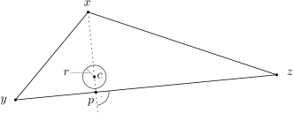
Figure 2: Illustration of the proof of Proposition 3.4

We can find a point $c$ in the interior of the triangle $\tau$, and a positive real number $r=r(\tau)$, such that for any point $v$ at a distance at most $r$ from $c$, the following holds:

1. $v$ is in the interior of $\tau$

2. the slope of the segment $vx$ differs from the slope of the segment $px$ (which is equal to $\eta+\pi/2$) by less than $\varepsilon$

3. the slope of the segment $vy$ differs from the slope of the segment $py$ (which is equal to $-\eta$) by less than $\varepsilon$

4. the slope of the segment $vz$ differs from the slope of the segment $pz$ (which is equal to $\eta$) by less than $\varepsilon$

Indeed, it suffices to choose $c$ sufficiently close to the point $p$ and set $r$ sufficiently small, and all the above conditions will be satisfied.

Consider now the embedding ${\cal{E}}_{T}$ of $T$. Place the center of the tripod on the point $c$, and scale the whole embedding by the factor $r$, so that it fits inside the triangle $\tau$. In view of the four conditions above, and in view of the seventh part of Lemma 3.8, it is not difficult to observe that we may rotate the (scaled) embedding of $T$ around the point $c$ by an integral multiple of $\varepsilon$ in such a way that every relevant vertex $v\in T$ has visibility towards all its neighbors among the three vertices $x,y,z$. Thus, we are able to embed all the necessary tilted edges of $G$ between $xyz$ and $T$ as straight line segments.

Note that in our embedding, all the balanced edges of $T$ have slopes from the set $S^{\prime}$, and all its internal faces are homothetic to the triangles from the set $R^{\prime}$. Furthermore, any tilted edge has one endpoint in the set $\{x,y,z\}$ and another endpoint in the set $c+rP^{\prime}$ (the set $P^{\prime}$ scaled $r$-fold and translated in such a way that the origin is moved to $c$). Hence any labelled tripod $T\in\text{Tr}(\Delta)$ can be inserted inside the triangle $xyz$ in such a way that the slopes of the edges always belong to the same finite set which depends on the triangle $xyz$ but not on the tripod $T$. Note that the triangle $xyz$ may be arbitrarily thin, in particular it can have inner angles smaller than $\varepsilon$.

Let us now show how the above construction yields an embedding of the whole graph $G$. For every such triangle $\tau\in R^{\prime}$, fix the point $c=c(\tau)$ and the radius $r=r(\tau)$ from the above construction. Any scaled and translated copy of $\tau$ will have the values of $c$ and $r$ scaled and translated accordingly.

We now embed the graph $G$ recursively, by embedding the outer face as an arbitrary triangle from $R^{\prime}$, and then recursively embedding each tripod into the appropriate face by the procedure described above. Since we only insert tripods into balanced faces, it is easily seen that every tripod is being embedded inside a triangle of $R^{\prime}$.

Overall, the construction uses at most $|S^{\prime}|={\cal O}(\Delta^{3})$ distinct slopes for the balanced edges, and at most $|R^{\prime}||P^{\prime}|={\cal O}(\Delta^{5})$ distinct slopes for the tilted edges. The total number of slopes is then ${\cal O}(\Delta^{5})$, as claimed. ∎

In the rest of this section, we prove the Tripod Drawing Lemma. Let $T$ be a labelled tripod and let $B$ be a bubble of $T$. Recall that the root edge of $B$ is the edge that belongs to a spine of $T$. Note that the same root edge is shared by two bubbles of $T$. Recall also that a bubble is called trivial if it only has two vertices.

We now introduce some terminology that will be convenient for our description of the structure of a given bubble.

Definition 3.9.

Let $B$ be a nontrivial bubble in a tripod $T$. The unique internal face of $B$ adjacent to its root edge will be called the root face of $B$. The dual of a bubble $B$ is the rooted binary tree ${\widehat{B}}$ whose nodes correspond bijectively to the internal faces of $B$, and two nodes are adjacent if and only if the corresponding faces of $B$ share an edge. The root of the tree ${\widehat{B}}$ is the node that represents the root face of $B$.

When dealing with the internal faces of $B$, we will employ the usual terminology of rooted trees; for instance, we say that a face $\Phi$ is the parent (or child) of a face $\Psi$ if the node representing $\Phi$ in ${\widehat{B}}$ is the parent (or child) of the node representing $\Psi$. For every internal face $\Phi$ of $B$, the three edges that form the boundary of $\Phi$ will be called the top edge, the left edge and the right edge, where the top edge is the edge that $\Phi$ shares with its parent face (or the root edge, if $\Phi$ is the root face), while left and right edges are defined in such a way that the top, left, and right edge form a counterclockwise sequence on the boundary of $\Phi$. With this convention, we may speak of a left child face or right child face of $\Phi$ without any ambiguity. Our terminology is motivated by the usual convention of embedding rooted binary trees with their root on the top, and the parent, the left child and the right child appearing in counterclockwise order around every node of the tree. Furthermore, for a given face $\Phi$, the bottom vertex of $\Phi$ is the common vertex of the left edge and right edge of $\Phi$.

Let us explicitly state the following simple fact which directly follows from our definitions.

Observation 3.10.

Let $\Phi_{1},\Phi_{2},\dotsc,\Phi_{k}$ be a sequence of internal faces of a bubble $B$, such that for any $j<k$, $\Phi_{j+1}$ is the left child of $\Phi_{j}$. Then all the faces $\Phi_{1},\dotsc,\Phi_{k}$ share a common vertex. In particular, if $B$ has maximum degree $\Delta$, then $k<\Delta$. An analogous observation holds for right children as well.

We now describe an approach that allows us to embed an arbitrary bubble with maximum degree $\Delta$ inside a bounded area using a bounded number of slopes.

Lemma 3.11.

Let $xyz$ be an equilateral triangle with vertex coordinates $x=(0,0)$, $y=(1,0)$ and $z=(1/2,-\sqrt{3}/2)$. Fix two sequences of slopes $\alpha_{1}$, $\alpha_{2}$, …, $\alpha_{\Delta-1}$ and $\beta_{1}$, $\beta_{2}$, …, $\beta_{\Delta-1}$, with $0>\alpha_{1}>\alpha_{2}>\dotsb>\alpha_{\Delta-1}>-\pi/3$ and $0<\beta_{1}<\beta_{2}<\dotsb<\beta_{\Delta-1}<\pi/3$. Let $S$ be the set of $2\Delta-1$ slopes $\{0\}\cup\{\alpha_{1},\alpha_{2},\dotsc,\alpha_{\Delta-1}\}\cup\{\beta_{1},\beta_{2},\dotsc,\beta_{\Delta-1}\}$. Let $B$ be a bubble of maximum degree $\Delta$. Then $B$ has a straight line embedding ${\cal{E}}_{B}$ inside $xyz$ that only uses the slopes from the set $S$, the root edge of ${\cal{E}}_{B}$ corresponds to the segment $xy$, and moreover the triangular faces of ${\cal{E}}_{B}$ form at most $2\Delta-3$ distinct triangles up to homothetic equivalence.

Proof.

Proceed by induction on the size of $B$. If $B$ is trivial, the statement holds. Assume now that $B$ is a nontrivial bubble. Let $\Phi_{0}$ be the root edge of $B$. See Figure 3.

Figure 3: Illustration of the proof of Lemma 3.11.

Define the maximal sequence of faces $\Phi_{1},\Phi_{2},\dotsc,\Phi_{\ell}$ in such a way that $\Phi_{i+1}$ is the left child of $\Phi_{i}$, with $\Phi_{1}$ being the left child of the root edge $\Phi_{0}$. The maximality of the sequence means that $\Phi_{\ell}$ has no left child. Symmetrically, define a maximal sequence of faces $\Psi_{1},\dotsc,\Psi_{r}$ such that $\Psi_{1}$ is the right child of $\Phi_{0}$, and $\Psi_{i+1}$ is the right child of $\Psi_{i}$. By Observation 3.10, we know that $\ell<\Delta-1$ and $r<\Delta-1$.

Let $(p,\alpha)$ denote the ray starting at a point $p$ and heading in direction $\alpha$.

Let $B$ be an arbitrary bubble. Let $v_{1}$ be the intersection of the rays $(x,\alpha_{1})$ and $(y,\beta_{1})$. The root face $\Phi_{0}$ will be embedded as the triangle $xyv_{1}$. Define points $v_{2},\dotsc,v_{\ell+1}$ by specifying $v_{i}$ as the intersection of $(x,\alpha_{i})$ and $(v_{1},\pi)$. The face $\Phi_{i}$ is then embedded as the triangle $xv_{i}v_{i+1}$. Similarly, define points $w_{2},\dotsc,w_{r+1}$ where $w_{i}$ is the intersection of $(y,\beta_{i})$ with $(v_{1},0)$. Then $\Psi_{1}$ is embedded as the triangle $yv_{1}w_{2}$, while for $k>1$ we embed $\Psi_{k}$ as the triangle $yw_{k}w_{k+1}$.

Note that when we remove the two vertices incident to the root edge from the bubble $B$, the remaining edges and vertices form a union of $\ell+r$ bubbles $B_{1}\cup\dotsb\cup B_{\ell}\cup B^{\prime}_{1}\cup\dotsc\cup B^{\prime}_{\ell}$, where $B_{i}$ is a bubble whose root edge is the right edge of $\Phi_{i}$ while $B^{\prime}_{j}$ is rooted at the left edge of $\Psi_{j}$. Using induction, we know that each $B_{i}$ has a straight line embedding inside the equilateral triangle whose top edge is the horizontal segment $v_{i}v_{i+1}$ (and symmetrically for $B^{\prime}_{j}$).

This completes the proof. ∎

Corollary 3.12.

Let $xyz$ be an arbitrary triangle and $B$ a bubble of maximum degree $\Delta$. There are sets $S$ of $2\Delta-1$ slopes and $R$ of $2\Delta-3$ triangles that depend on $xyz$ but not on $B$, such that $B$ can be embedded inside $xyz$ using only slopes from $S$ and triangles from $R$ for triangular faces, in such a way that the root edge of $B$ coincides with the segment $xy$.

Proof.

This follows from Lemma 3.11, using the fact that for any triangle there is an affine transform that maps it to an equilateral triangle, and that affine transforms preserve the number of distinct slopes used in a straight-line embedding. ∎

The construction from Lemma 3.11 can be applied to embed all the irrelevant bubbles of a given labelled tripod $T$. Unfortunately, the construction of Lemma 3.11 is not suitable for the embedding of relevant bubbles, because it provides no control about the position of the relevant vertices. Indeed, inside the triangle $xyz$ of the previous lemma, there are infinitely many points where a vertex may be embedded by the construction described in the proof of the lemma. Thus, we can give no upper bound on the number of potential embeddings of relevant vertices.

For this reason, we now describe a more complicated embedding procedure, which allows us to control the position of the relevant vertices. We first need some auxiliary definitions.

Definition 3.13.

An adder $A$ is a bubble with a root edge $h$ and another edge $t\neq h$, such that the dual tree of $A$ is a path, and the edge $t$ is an external edge adjacent to the single leaf face of $A$. See Figure 4. The edges $h$ and $t$ are called head and tail of the adder. It is easy to see that every adder contains a unique path $Z$ whose first edge is $h$, its last edge is $t$ and no other edge of $Z$ belongs to the outer face of $A$. The path $Z$ will be called the zigzag path of the adder $A$. The length of the adder is defined to be the number of edges of its zigzag path. By definition, each adder has length at least 2. An adder of length 2 will be called degenerate.

Figure 4: An adder. The bold edges form the zigzag path.

We will now show that adders of bounded degree can be embedded inside a prescribed quadrilateral using a bounded number of slopes and triangles.

Lemma 3.14.

For every convex quadrilateral $Q=abcd$ and for every $\Delta$ there is a set $S$ of ${\cal O}(\Delta)$ slopes, a set $S_{0}\subseteq S$ of ${\cal O}(1)$ slopes, and a set $R$ of ${\cal O}(\Delta)$ triangles such that any nondegenerate adder $A$ of maximum degree $\Delta$ has a straight line embedding ${\cal{E}}_{A}$ with the following properties:

1. All the edge-slopes of ${\cal{E}}_{A}$ belong to the set $S$.

2. All the edges on the outer face of ${\cal{E}}_{A}$ have slopes from the set $S_{0}$.

3. Each internal face of ${\cal{E}}_{A}$ is homothetic to a triangle from $R$.

4. The head of $A$ coincides the edge $ab$ of $Q$ and the tail of $A$ coincides with $cd$.

5. The embedding ${\cal{E}}_{A}$ is contained in the convex hull of $abcd$.

Proof.

Note that the lemma is clearly true when restricted to adders of length at most four (or any other bounded length). In the rest of the proof, we assume that $A$ is an adder of length at least five.

We first deal with the case when the edges $ab$ and $cd$ are parallel (i.e., $Q$ is a trapezoid), and the adder $A$ has odd length $\ell=2k+1$. Without loss of generality, assume that the segments $ab$ and $cd$ are horizontal and that the line containing $cd$ is above the line containing $ab$. Let $\alpha$ be the slope of the diagonal $ac$ and $\beta$ the slope of the diagonal $bd$, with $0<\alpha<\beta<\pi$. Let $e$ be the point where the two diagonals intersect. Notice that the two triangles $abe$ and $cde$ are homothetic. Let $r=\|ab\|/\|cd\|=\|ae\|/\|ce\|$ be the dilation factor of the homothecy.

Let $Z$ be the zigzag path of $A$. Let us identify the head of $A$ with the segment $ab$ and the tail of $A$ with $cd$, in such a way that the cyclic order of the four points $abcd$ on the boundary of $Q$ is the same as the cyclic order in which the corresponding vertices appear on the outer face of $A$.

Figure 5: Embedding an adder with prescribed head and tail. These figures illustrates the embedding of the adder of odd length $2k+1$. The two figures correspond to the two cases depending on the parity of $k$.

Since $A$ has odd length, the endpoints of its zigzag path are diagonally opposite in $Q$, see Figure 5. We lose no generality by assuming that $a$ and $c$ are the endpoints of the zigzag path. Let $v_{0},v_{1},v_{2},\dotsc,v_{k},w_{k},w_{k-1},w_{k_{2}},\dotsc,w_{1},w_{0}$ be the sequence of the vertices of $Z$, in the order in which they appear on the path $Z$, with $v_{0}=a$, $v_{1}=b$, $w_{0}=c$, and $w_{1}=d$. Fix an arbitrary slope $\gamma$ such that $\beta<\gamma<\pi$. All the vertices of $Z$ will be embedded on the two diagonals $ac$ and $bd$. Since the first two and last two vertices have already been embedded, let us proceed by induction, separately in each half of $Z$. If, for some $i\geq 0$, the vertex $v_{i}$ has already been embedded on the diagonal $ac$, then we embed $v_{i+1}$ on $bd$ in such a way that the segment $v_{i}v_{i+1}$ is horizontal. If $v_{i}$ has been embedded on the diagonal $bd$, then $v_{i+1}$ is embedded on $ac$ and the slope of $v_{i}v_{i+1}$ is equal to $\gamma$.

We proceed similarly with the vertices $w_{i}$: if $w_{i}$ is on $ac$ then $w_{i+1}$ is on $bd$ and the segment $w_{i}w_{i+1}$ has slope $\gamma$; otherwise $w_{i}$ is on $bd$ and $w_{i+1}$ is on $ac$ and the corresponding segment is horizontal.

We may easily show by induction that for any $i$, the triangles $ev_{i}v_{i+1}$ and $ew_{i}w_{i+1}$ are similar, all of them with the same ratio $r=\|ev_{i}\|/\|ew_{i}\|$. Furthermore, we see that $ev_{i}v_{i+1}$ is similar to $ev_{i+2}v_{i+3}$, with a ratio $q$ that is independent of $i$. From these facts, we see that all the segments of the form $v_{i}w_{i+1}$ have at most two distinct slopes (depending on the parity of $i$), and similarly for the segments of the form $w_{i}v_{i+1}$.

Let us consider all the triangles formed by triples of vertices $xyz$ where $x,y$ and $z$ are three consecutive vertices of the path $Z$. Note that these triangles are internally disjoint, and their edges form at most six distinct slopes, namely $0,\alpha,\beta,\gamma$, the slope of the segment $v_{k}w_{k-1}$ and the slope of the segment $v_{k-1}w_{k}$. Furthermore, the latter two slopes belong to a set of at most four slopes that are independent of $k$, and hence independent of the adder $A$. The union of the above-described triangles will form the outer boundary of our embedding of $A$. It remains to place the vertices of $A$ that do not belong to $Z$ to this boundary.

Let us fix $\Delta-2$ additional slopes $\gamma_{1}<\gamma_{2}<\dotsb<\gamma_{\Delta-2}$ which are all greater than $\gamma$ but smaller than $\pi$. Note than any vertex $u$ of $A$ that does not belong to $Z$ is incident to exactly one edge that does not belong to the outer face of $A$, and this edge connects $u$ to a vertex of $Z$. Thus, to complete the description of the embedding of $A$, it suffices to specify, for every vertex $v$ of $Z$, the slopes of all the edges that do not belong to the outer face of $A$ and that connect $v$ to a vertex not belonging to $Z$. Thus, let us fix an arbitrary vertex $v$ of $Z$. Let us assume that $v$ has been embedded on the diagonal $ac$ and that $v=v_{i}$ for some $i\leq k$ (the cases when $v$ belongs to $bd$ or $v=w_{i}$ are analogous). Let $u_{1},\dotsc,u_{\ell}$ be the vertices not belonging to $Z$ and adjacent to $v$ by an internal edge of $A$. Note that if $v$ has at least one such neighbor $u_{i}$, then $v\neq v_{1}$, because $v_{1}$ is not incident to any edge not belonging to the outer face. Let $v^{+}$ be the vertex that follows after $v$ on $Z$ (typically, $v^{+}=v_{i+1}$, unless $v=v_{k}$, when $v^{+}=w_{k}$). Assume that the vertices $u_{1},\dotsc u_{\ell}$ are listed in their counterclockwise order with respect to the neighborhood of $v$. Let us place each $u_{i}$ at the intersection of the line $v_{i-1}v^{+}$ and the ray $(v,\pi+\gamma_{i})$. This choice guarantees that the edge $vu_{i}$ has slope $\gamma_{i}$.

We have thus found a straight line embedding of $A$ that has all the required properties and uses at most $\Delta+{\cal O}(1)$ slopes. This completes the case when $A$ is an odd-length adder and $Q$ is a trapezoid.

Assume now that $A$ is an arbitrary nondegenerate adder of length $\ell\geq 5$, and $Q$ is an arbitrary convex quadrilateral. Our goal is to reduce this situation to the cases solved above. Note that the adder $A$ can be written as a union of two non-degenerate sub-adders $A_{1}$ and $A_{2}$, where $A_{1}$ has odd length, $A_{2}$ has length three or four, $A_{1}$ has the same head as $A$, $A_{2}$ has the same tail as $A$, the tail of $A_{1}$ is the head of $A_{2}$, and the adders $A_{1}$ and $A_{2}$ are otherwise disjoint. Accordingly, the convex quadrilateral $Q=abcd$ can be decomposed into a union of two internally disjoint quadrilaterals $Q_{1}=abc^{\prime}d^{\prime}$ and $Q_{2}=d^{\prime}c^{\prime}cd$, where $Q_{1}$ is a trapezoid. We may now use our previous arguments to construct an embedding of $A_{1}$ inside $Q_{1}$, and an embedding of $A_{2}$ inside $Q_{2}$, and combine the two embeddings into an embedding of $Q$ satisfying the conditions of the lemma. ∎

We will use adders as basic building blocks in a procedure that embeds any given bubble with prescribed relevant vertices in such a way that the embedding of all the relevant vertices is chosen from a finite set of points. The following technical lemma summarizes all the key properties of the bubble embedding that we are about to construct.

Lemma 3.15.

Let $T=abc$ be an isosceles triangle with base $ab$, and with internal angles $\varepsilon/2,\varepsilon/2$ and $\pi-\varepsilon$. Assume that the line $ab$ is horizontal and the point $c$ is below the line $ab$. For every $\Delta>0$ there is a set $S$ of ${\cal O}(\Delta^{3})$ slopes, a set $P$ of ${\cal O}(\Delta)$ points, and a set $R$ of ${\cal O}(\Delta^{3})$ triangles, such that every labelled bubble $B\in{\cal{B}}(\Delta)$ has an embedding ${\cal{E}}_{B}$ with the following properties.

1. All the edge-slopes of ${\cal{E}}_{B}$ belong to $S$.

2. Any relevant vertex of $B$ is embedded at a point from $P$.

3. Every internal face of ${\cal{E}}_{B}$ is homothetic to a triangle from $R$.

4. The root edge of $B$ coincides with the segment $ab$.

5. The whole embedding ${\cal{E}}_{B}$ is inside the triangle $T$.

6. Any relevant vertex of ${\cal{E}}_{B}$ has visibility in any direction from the set $\langle\pi+\varepsilon,2\pi-\varepsilon\rangle$.

Proof.

Let us first introduce some terminology (see Figure 6). Let $B\in{\cal{B}}(\Delta)$ be a labelled bubble. Recall from Definition 3.9 that the dual of $B$, denoted by ${\widehat{B}}$, is a rooted binary tree whose root corresponds to the root face of $B$. For an internal face $\Phi$ of $B$, we let ${\widehat{\Phi}}$ denote the corresponding node of ${\widehat{B}}$. We distinguish several types of nodes in ${\widehat{B}}$. A node ${\widehat{\Phi}}$ is called relevant node, if the bottom vertex of the face $\Phi$ is a relevant vertex of $B$. A node ${\widehat{\Phi}}$ of ${\widehat{B}}$ is called peripheral if the subtree of ${\widehat{B}}$ rooted at ${\widehat{\Phi}}$ does not contain any relevant node, in other words, neither ${\widehat{\Phi}}$ nor any descendant of ${\widehat{\Phi}}$ is relevant. A node is central if it is not peripheral. Note that the central nodes induce a subtree of ${\widehat{B}}$; we let ${\widehat{B}}^{\prime}$ denote this subtree. By construction, all the leaves of ${\widehat{B}}^{\prime}$ are relevant nodes (but there may be relevant nodes that are not leaves).

Figure 6: An example of a labelled bubble $B$ with its dual tree ${\widehat{B}}$. Relevant vertices are represented by large black disks. The large gray disks of the bottom figure represent the non-relevant priority vertices.

A node ${\widehat{\Phi}}$ of ${\widehat{B}}^{\prime}$ is a branching node if both its children belong to ${\widehat{B}}^{\prime}$ as well. A node of ${\widehat{B}}^{\prime}$ is a connecting node if it is neither relevant nor branching. By definition, each connecting node has a unique child in ${\widehat{B}}^{\prime}$, and the connecting nodes induce in ${\widehat{B}}^{\prime}$ a disjoint union of paths. We call these paths the connections.

We say that a face $\Phi$ of $B$ is al relevant face if the corresponding node ${\widehat{\Phi}}$ is a relevant node. Peripheral faces, branching faces and connecting faces are defined analogously. Let $B^{\prime}$ be the subgraph of $B$ whose dual is ${\widehat{B}}^{\prime}$. If ${\widehat{B}}^{\prime}$ is empty, define $B^{\prime}$ to be the trivial bubble consisting of the root edge of $B$. In any case, $B^{\prime}$ is a subbubble of $B$ and has the same root edge as $B$.

Note that since every leaf of ${\widehat{B}}^{\prime}$ is a relevant node, and since $B$ has at most $3\Delta$ relevant vertices by definition of ${\cal{B}}(\Delta)$, the tree ${\widehat{B}}^{\prime}$ has at most ${\cal O}(\Delta)$ leaves and consequently at most ${\cal O}(\Delta)$ branching nodes.

Let us now describe the basic idea of the proof. We begin by specifying the set $P$ of points. The points of $P$ will form a convex cup inside the triangle $T$. For a given bubble $B\in{\cal{B}}(\Delta)$, we construct the embedding ${\cal{E}}_{B}$ in three steps. In the first step, we take all the vertices of $B$ that belong to relevant faces and branching faces, and embed them to the points of $P$. In the second step, we embed all the connecting faces. Each connection in ${\widehat{B}}^{\prime}$ corresponds to a (possibly degenerate) adder contained in $B^{\prime}$, whose head and tail have been embedded in the first step. Using the construction from Lemma 3.14, we insert these adders into the embedding. Thus, in the first two steps, we construct an embedding of $B^{\prime}$. In the third step, we extend this embedding into an embedding of $B$ by adding the peripheral faces. These faces form a disjoint union of subbubbles, each of them rooted at an edge belonging to the outer face of $B^{\prime}$. We use Corollary 3.12 to embed each of these subbubbles into a thin triangle above a given root edge.

Let us describe the individual steps in detail. Set $D=18\Delta$. Recall that $T$ is an isosceles triangle with base $ab$. Let $C$ be any circular arc with endpoints $a$ and $b$, drawn inside $T$. Choose a sequence $p_{1},p_{2},\dotsc,p_{D}$ of distinct points of $C$, in such a way that $p_{1}=a$, $p_{D}=b$, and the remaining points are chosen arbitrarily on $C$ in order to form a left-to-right sequence. Let $P$ be the set $\{p_{1},\dotsc,p_{D}\}$.

Let us say that a vertex $v$ of $B$ is a priority vertex if it either belongs to a relevant face, or it belongs to a branching face, or it belongs to the root edge of $B$. Note that all priority vertices actually belong to $B^{\prime}$, and that each relevant vertex is a priority vertex as well. Let $\ell$ be the number of priority vertices. We know that $B$ has at most $3\Delta$ relevant faces. Since every leaf of ${\widehat{B}}^{\prime}$ represents a relevant face, we see that $B^{\prime}$ has at most $3\Delta-1$ branching faces. This implies that $\ell<D=18\Delta$.

Let $v_{1},v_{2},\dotsc,v_{\ell}$ be the sequence of all the priority vertices of $B$, listed in counterclockwise order of their appearance on the outer face of $B$, in such a way that $v_{1}$ and $v_{\ell}$ are the vertices of the root edge of $B$. For each $i\in\{1,\dotsc,\ell-1\}$, we embed the vertex $v_{i}$ on the point $p_{i}$, while the vertex $v_{\ell}$ is embedded on the point $v_{D}=b$. Note that this embedding guarantees that the root edge of $B$ coincides with the segment $ab=p_{1}p_{D}$. Moreover, since this embedding preserves the cyclic order of the vertices on the boundary of the outer face, we know that the edges induced by the priority vertices do not cross. This completes the first step of the embedding.

In the second step, we describe the embedding of the connecting faces of $B$. Let $\Phi_{1},\Phi_{2},\dotsc,\Phi_{k}$ be a sequence of faces of $B$ corresponding to a connection in ${\widehat{B}}$, where we assume that for each $i<k$, the node ${\widehat{\Phi}}_{i}$ is the parent of ${\widehat{\Phi}}_{i+1}$ in ${\widehat{B}}$. See Figure 7. Let $x$ be the left vertex of $\Phi_{1}$ and let $y$ be the right vertex of $\Phi_{1}$. The vertices $x$ and $y$ either form the root edge of $B$, or they belong to the parent face of $\Phi_{1}$, which is either a relevant face or a branching face. In either case, both $x$ and $y$ are priority vertices. In particular, $x$ corresponds to a point $p_{m}\in P$, and $y$ corresponds to $p_{n}\in P$, for some $m<n$.

Figure 7: An adder representing a connection in ${\widehat{B}}$.

Consider now the face $\Phi_{k}$. Since it is neither relevant nor branching, it has a unique child face $\Phi^{\prime}$ in $B^{\prime}$. The face $\Phi^{\prime}$ is relevant or branching, so all its vertices are priority vertices. Let $u$ be the left vertex of $\Phi^{\prime}$ and let $v$ be its right vertex. The edge $uv$ is the intersection of $\Phi^{\prime}$ and $\Phi_{k}$. Let $A$ be the adder formed by the union of the faces $\Phi_{1},\dotsc,\Phi_{k}$, with head $xy$ and tail $uv$. Note that this adder does not contain any other priority vertices apart from $x$, $y$, $u$ and $v$. In particular, the vertex $u$ is either equal to $x$, or it corresponds to $p_{m+1}$. For the vertex $v$, we have three possibilities: either $v=y$, or $v=p_{n-1}$, or $v=p_{\ell-1}$ and $y=p_{D}$.

Let us first deal with the case when the adder $A$ is degenerate, i.e., either $x=u$ or $y=v$. We first define a set $Q$ of auxiliary points (see Figure. 8. For every $i<D$, consider the segment $p_{i}p_{i+1}$, and subdivide this segment with $\Delta-2$ new points $q^{i}_{1},q^{i}_{2},\dotsc,q^{i}_{\Delta-2}$. Next, for $i<D-1$, consider also the segment $p_{i}p_{D}$ and subdivide it with $\Delta-2$ points $\tilde{q}^{i}_{1},\tilde{q}^{i}_{2},\dotsc,\tilde{q}^{i}_{\Delta-2}$. Let $Q$ be the set of all the points $q_{j}^{i}$ and $\tilde{q}_{j}^{i}$, for all $i$ and $j$.

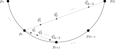
Figure 8: The auxiliary points from the set $Q$.

Assume now that $A$ is a degenerate adder with $x=u$ (the case when $y=v$ is analogous). Recall that $A$ has $k$ internal faces $\Phi_{1},\dotsc,\Phi_{k}$. All these faces share the vertex $x$, and in particular, $x$ has degree $k+1$ in $A$. This shows that $k<\Delta$, and consequently there are at most $\Delta-2$ non-priority vertices in $A$, all of them on a path from $v$ to $y$. See Figure 9. If $v=p_{n-1}$, we embed these non-priority vertices on the points $q_{1}^{n-1},\dotsc,q_{k-1}^{n-1}$. On the other hand, if $v=p_{\ell-1}$ and $y=p_{D}$, we embed the non-priority vertices of $A$ on the points $\tilde{q}_{1}^{\ell-1},\dotsc,\tilde{q}_{k-1}^{\ell-1}$. This determines the embedding of $A$.

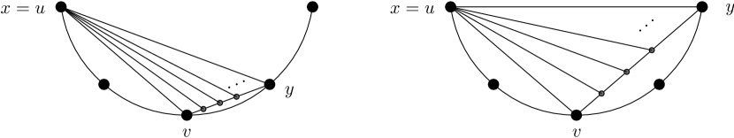
Figure 9: The embedding of a degenerate connection adder.

Consider now the case when $A$ is non-degenerate. The four vertices $x$, $y$, $u$ and $v$ form a convex quadrilateral, and we embed $A$ inside this quadrilateral, using the construction of Lemma 3.14. This again determines the embedding of $A$.

Using the constructions described above, we embed all the adders representing connections in ${\widehat{B}}$. Note that each adder is embedded inside the convex hull of its head and tail. Moreover, if $A$ and $A^{\prime}$ are adders representing two different connections, the convex hull of the head and tail of $A$ is disjoint from the convex hull of the head and tail of $A^{\prime}$, except for at most one vertex shared by the two adders. This shows that the embedding is indeed a plane embedding of the graph $B^{\prime}$, completing the second step of the construction.

Before we describe the last step, let us estimate the number of vertices, edge-slopes and internal faces that may arise in the first two steps. Clearly, any relevant vertex is embedded on a point from the set $P$, which has size ${\cal O}(\Delta)$ and does not depend on the bubble $B$.

Any edge $e$ embedded in the first two steps may have one of the following forms.

• The edge $e$ connects two points from $P$. Such edges can take at most ${\cal O}(\Delta^{2})$ slopes.

• The edge $e$ connects a vertex from $P$ to a vertex from $Q$. This yields ${\cal O}(\Delta^{3})$ possible slopes.

• The edge $e$ connects two vertices of $Q$. This is only possible when both vertices of $e$ belong to a segment determined by a pair of points in $P$. The slope of $e$ is then equal to a slope determined by two points from $P$.

• The edge $e$ belongs to a non-degenerate adder $A$ representing a connection in $B$. In the embedding from Lemma 3.14, the edges of a given adder $A$ determine at most ${\cal O}(\Delta)$ slopes, and these slopes only depend on the four vertices forming the head and tail of $A$. This fourtuple of vertices has the form $\{p_{i},p_{i+1},p_{j-1},p_{j}\}$ or $\{p_{i},p_{i+1},p_{j-1},p_{D}\}$. There are ${\cal O}(\Delta^{2})$ such fourtuples and hence ${\cal O}(\Delta^{3})$ possible slopes for the edges of this type.

Overall, there is a set of ${\cal O}(\Delta^{3})$ slopes, independent of $B$, such that any edge embedded in the first two steps has one of these slopes.

Next, we count homothecy types of internal faces. Any internal face $\Phi$ embedded in the first two steps has one of the following types.

• All the vertices of $\Phi$ belong to $P$. There are ${\cal O}(\Delta^{3})$ such faces.

• $\Phi$ has two vertices from $P$ and one vertex from $Q$. In such case the triple of vertices of $\Phi$ must be of one of these forms, for some values of $i$, $j$ and $k$: $\{p_{i},p_{j},q^{j}_{1}\}$, or $\{p_{i},p_{j},q^{j-1}_{k}\}$, or $\{p_{i},p_{D},\tilde{q}^{j}_{k}\}$. There are ${\cal O}(\Delta^{3})$ such triples.

• $\Phi$ has two vertices from $Q$ and one vertex from $P$. In such case the two vertices from $Q$ are of the form $\{q_{j}^{i},q_{j+1}^{i}\}$ or $\{\tilde{q}_{j}^{i},\tilde{q}_{j+1}^{i}\}$ for some $i$ and $j$. This again gives ${\cal O}(\Delta^{3})$ possibilities for $\Phi$.

• $\Phi$ is an internal face of a non-degenerate adder, embedded by Lemma 3.14. Lemma 3.14 shows that the internal faces of such an adder form ${\cal O}(\Delta)$ homothecy types depending only on the position of head and tail. Since there are ${\cal O}(\Delta^{2})$ positions for head and tail, this gives ${\cal O}(\Delta^{3})$ triangle types up to homothecy.

We conclude that each internal face of $B^{\prime}$ is homothetic to one of ${\cal O}(\Delta^{3})$ triangles, and these triangles do not depend on $B^{\prime}$.

We next estimate the number of slopes formed by edges on the outer face of $B^{\prime}$. For $e$ on the outer face of $B^{\prime}$ there are two possibilities.

• If both endpoints of $e$ are priority vertices, or if $e$ belongs to a connection represented by a degenerate adder, then the line determined by the segment $e$ passes through two points of $P$. In particular, such a segment $e$ must have one of ${\cal O}(\Delta^{2})$ slopes determined by $P$.

• Suppose $e$ belongs to the outer face of a non-degenerate adder $A$. By Lemma 3.14, the edges of the outer face of $A$ have ${\cal O}(1)$ distinct slopes, depending on the head and tail of $A$. Overall, such edges have at most ${\cal O}(\Delta^{2})$ slopes.

This shows that the slopes of the edges of the outer face of $B^{\prime}$ all belong to a set of ${\cal O}(\Delta^{2})$ slopes.

To finish the proof, it remains to perform the third step of the construction, where we embed the peripheral faces. Fix an angle $\delta>0$ such that $\delta<\varepsilon/2$ and any two distinct edge-slopes used in the first two steps of the construction differ by more than $2\delta$. Let $e$ be an edge of the outer face of $B^{\prime}$. Let $T_{e}$ be an isosceles triangle whose base is the edge $e$, whose internal angles have size $\delta$, $\delta$, and $\pi-2\delta$, and which lies in the outer face of $B^{\prime}$. It is easy to check that our choice of $\delta$ guarantees that for any two edges $e$ and $f$ on the outer face of $B^{\prime}$, the triangles $T_{e}$ and $T_{f}$ are disjoint, except for a possible common vertex of $e$ and $f$.

Let ${\widehat{B}}_{0}$ be a maximal subtree of ${\widehat{B}}$ formed entirely by peripheral nodes, and let $B_{0}$ be the dual of ${\widehat{B}}_{0}$. Note that $B_{0}$ is a subbubble of $B$ rooted at an edge of the outer face of $B^{\prime}$. Let $e$ be the root edge of $B_{0}$. Using Corollary 3.12, we embed $B_{0}$ inside $T_{e}$, in such a way that the root edge of $B_{0}$ coincides with $e$. This embedding of $B_{0}$ uses ${\cal O}(\Delta)$ edge-slopes and ${\cal O}(\Delta)$ triangle types for its internal faces, and these edge-slopes and triangle types only depend on the slope of $e$.

Since the edges on the outer face of $B^{\prime}$ may have at most ${\cal O}(\Delta^{2})$ edge-slopes, we may embed all the peripheral faces of $B$, while using only ${\cal O}(\Delta^{3})$ edge-slopes and ${\cal O}(\Delta^{3})$ triangle types in addition to the edge-slopes and triangle types used in the first two steps of the construction.

This completes the last step of the construction. It is easy to check that in the obtained embedding of $B$, any relevant vertex has visibility in any direction from the set $\langle\pi+\varepsilon,2\pi-\varepsilon\rangle$, and the remaining claims of the lemma have already been verified. ∎

At last, we are ready to give the proof of the Tripod Drawing Lemma. Let us recall its statement:

Lemma 3.8 (repeated).

For every $\Delta$ there is a set of slopes $S$ of size ${\cal O}(\Delta^{3})$, a set of points $P$ of size ${\cal O}(\Delta^{2})$, and a set of triangles $R$ of size ${\cal O}(\Delta^{3})$, such that every labelled tripod $T\in\text{Tr}(\Delta)$ has a straight-line embedding ${\cal{E}}_{T}$ with the following properties:

1. The slope of any edge in the embedding ${\cal{E}}_{T}$ belongs to $S$.

2. Each relevant vertex of ${\cal{E}}_{T}$ is embedded on a point from $P$.

3. Each internal face of ${\cal{E}}_{T}$ is homothetic to a triangle from $R$.

4. The central vertex of ${\cal{E}}_{T}$ is embedded in the origin of the plane.

5. Any vertex of ${\cal{E}}_{T}$ is embedded at a distance at most $1$ from the origin.

6. Each spine of $T$ is embedded on a single ray starting from the origin. The three rays containing the spines have directed slopes $0$, $2\pi/3$ and $4\pi/3$. Let these three rays be denoted by $r_{1}$, $r_{2}$ and $r_{3}$, respectively.

7. Let ${\widehat{r_{i}r_{j}}}$ denote the closed convex region whose boundary is formed by the rays $r_{i}$ and $r_{j}$. Any relevant vertex of ${\cal{E}}_{T}$ embedded in the region ${\widehat{r_{1}r_{2}}}$ (or ${\widehat{r_{2}r_{3}}}$, or ${\widehat{r_{1}r_{3}}}$) has visibility in any direction from the set $\langle\varepsilon,2\pi/3-\varepsilon\rangle$ (or $\langle 2\pi/3+\varepsilon,4\pi/3-\varepsilon\rangle$, or $\langle 4\pi/3+\varepsilon,2\pi-\varepsilon\rangle$, respectively).

   Note that the three regions ${\widehat{r_{1}r_{2}}}$, ${\widehat{r_{2}r_{3}}}$ and ${\widehat{r_{1}r_{3}}}$ are not disjoint. For instance, if a relevant vertex of $T$ is embedded on the ray $r_{1}$, it belongs to both ${\widehat{r_{1}r_{2}}}$ and ${\widehat{r_{1}r_{3}}}$, and hence it must have visibility in any direction from the set $\langle\varepsilon,2\pi/3-\varepsilon\rangle\cup\langle 4\pi/3+\varepsilon,2\pi-\varepsilon\rangle$.

Proof.

Fix a tripod $T\in\text{Tr}(\Delta)$. Let $X$, $Y$, and $Z$ be the three legs of the tripod $T$. The center $c$ of the tripod will coincide with the origin of the coordinate system, and the spines of the three legs will be embedded onto three rays with slopes $0$, $2\pi/3$ and $4\pi/3$ starting at the origin. We will now describe how to embed the leg $X$ onto the horizontal ray $(c,0)$. The embeddings of the remaining two legs are then built by an analogous procedure, rotated by $2\pi/3$ and $4\pi/3$.

Let $X$ be a fixed leg of the tripod, represented as a sequence $D_{1},D_{2},\dotsc,D_{k}$ of double bubbles, ordered from the center outwards. Recall that a bubble is called relevant if it contains at least one relevant vertex. We will also say that a double bubble is relevant if at least one of its two parts is relevant.

Define a parameter $D$ by $D=13\Delta$. The leg $X$ can have at most $6\Delta$ relevant double bubbles. A maximal consecutive sequence of the form $D_{i},D_{i+1},\dotsc,D_{j}$ in which each element is an irrelevant double bubble will be called an irrelevant run. We partition $X$ into a sequence of parts $P_{1},P_{2},\dotsc,P_{\ell}$, where a part is either a single relevant double bubble, or a nonempty irrelevant run. Since by definition no two irrelevant runs are consecutive, we see that $X$ has at most $12\Delta+1<D$ parts.

Let $T_{\varepsilon}$ be an isosceles triangle with internal angles of size $\varepsilon/2$, $\varepsilon/2$ and $\pi-\varepsilon$ whose base edge is horizontal. From Lemma 3.15, we know that there is a set of points $P_{\varepsilon}\subset T_{\varepsilon}$ of size ${\cal O}(\Delta)$, a set of slopes $S_{\varepsilon}$ of size ${\cal O}(\Delta^{3})$ and set of triangles $R_{\varepsilon}$ of size ${\cal O}(\Delta^{3})$ such that any bubble of $B\in{\cal{B}}(\Delta)$ can be embedded inside $T_{\varepsilon}$ using slopes from $S_{\varepsilon}$ in such a way that each relevant vertex of $B$ coincides with a point from the set $P_{\varepsilon}$ and the internal faces of the embedding are homothetic to triangles in $R$. Let ${\cal{E}}_{B}$ denote this embedding.

We will combine these embeddings to obtain an embedding of the whole leg $X$. To each of the at most $D$ parts of $X$ we will assign a segment of length $L=\frac{1}{D}$ on the horizontal ray $(c,0)$.

Assume first that $P_{i}$ is a part of $X$ consisting of a single relevant double bubble, formed by a pair of bubbles $B$ and $C$. We will embed $P_{i}$ in such a way that the common root edge of $B$ and $C$ coincides with a horizontal segment $e_{i}$ of length $L$, whose endpoints have horizontal coordinates $(i-1)L$ and $iL$. The two bubbles $B$ and $C$ are then embedded inside two scaled and translated copies of $T_{\varepsilon}$ that share a common base $e_{i}$, using the embeddings ${\cal{E}}_{B}$ and ${\cal{E}}_{C}$, possibly reflected along the horizontal axis.

Now assume that $P_{i}$ is a part of $X$ that consists of an irrelevant run of $k$ irrelevant double bubbles $D_{j},D_{j+1},\dotsc,D_{i+k-1}$. We embed the root edge of each double bubble onto a segment of length $L/k$, and embed the rest of the double bubble into a scaled and translated copy of $T_{\varepsilon}$. We then concatenate these embeddings to obtain an embedding of the whole irrelevant run, which will occupy a segment of length exactly $L$ on the spine of $X$.

Overall, since the leg has at most $D$ parts, the whole leg will be embedded at distance at most 1 from the origin. It is easy to see that the embedding of $X$ uses at most $2|S_{\varepsilon}|$ slopes and $2|R_{\varepsilon}|$ triangles for faces (up to scaling). The embedding of the whole tripod will then require at most $6|S_{\varepsilon}|={\cal O}(\Delta^{3})$ slopes and $6|R_{\varepsilon}|={\cal O}(\Delta^{3})$ non-homothetic triangles.

Let us estimate the number of possible points where a relevant vertex may be embedded. For every relevant double bubble, there are at most $D$ possibilities where its root edge may be embedded within the embedding of $X$. Since a bubble may be either above or below the spine, each relevant bubble has at most $2D$ possibilities where it may appear within $X$, and at most $6D$ possibilities within the whole tripod. As soon as we fix the embedding of the root edge and the relative position of the bubble with respect to its spine, we are left with at most $|P_{\varepsilon}|$ possibilities where a relevant vertex may be embedded. There are overall at most $6D|P_{\varepsilon}|={\cal O}(\Delta^{2})$ possible embeddings of relevant vertices.

Using Lemma 3.15, it is straightforward to check that the embedding satisfies the required visibility properties. Lemma 3.8 (and hence also Proposition 3.4 and Theorem 1.1) is now proved. ∎

4 Series-parallel graphs of maximum degree 3

In this section, we prove Theorem 1.2, which states that each series-parallel graph of maximum degree at most 3 has planar slope number at most 3. This bound is optimal, since it is not difficult to see that, e.g., the complete bipartite graph $K_{2,3}$, which is series-parallel, cannot be embedded with fewer than 3 slopes.

We will in fact show that any series-parallel graph with $\Delta\leq 3$ can be embedded using the slopes from the set $S=\{0,\pi/4,-\pi/4\}$. This particular choice of $S$ is purely aesthetic, since for any other set $S^{\prime}$ of three slopes there is an affine bijection of the plane that maps segments with slopes from $S^{\prime}$ to segments with slopes from $S$. Thus, any plane graph that has an embedding with three distinct slopes also has an embedding with the slopes from the set $S$.

Throughout this section, segments of slope $\pi/4$ (or 0, or $-\pi/4$) will be known as increasing (or horizontal, or decreasing, respectively).

Let us first define series-parallel graphs.

A two-terminal graph $(G,s,t)$ is a graph together with two distinct prescribed vertices $s,t\in V(G)$, known as terminals. The vertex $s$ is called source and $t$ is called sink.

For a sequence $(G_{1},s_{1},t_{1}),(G_{2},s_{2},t_{2}),\dotsc,(G_{k},s_{k},t_{k})$ of two-terminal graphs, we define the serialization of the sequence to be the two-terminal graph $(G,s_{1},t_{k})$ obtained by identifying, for every $i\in\{1,\dotsc,k-1\}$ the vertex $t_{i}$ with the vertex $s_{i+1}$. The parallelization of the sequence of two-terminal graph is the two-terminal graph $(H,s,t)$ obtained by identifying all the sources $s_{i}$ into a single vertex $s$ and all the sources $t_{i}$ into a single vertex $t$. Whenever we perform parallelization of a sequence of graphs, we assume that at most one graph of the sequence contains the edge from source to sink. Thus, the result of a parallelization is again a simple graph. Serialization and parallelization will be jointly called SP-operations.

A two-terminal graph $(G,s,t)$ is called series-parallel graph or SP-graph for short, if it either consist of a single edge connecting the vertices $s$ and $t$, or if it can be obtained from smaller SP-graphs by an SP-operation.

If follows from the definition, that SP-graphs can be constructed from single edges by repeated serializations and parallelizations. In general, this construction is not unique. E.g., a path of length four whose endpoints are the terminals can be constructed as a serialization of four edges, or as a serialization of two paths of length two.

It is often convenient to employ special type of SP-operation that makes the construction of an SP-graph unique. To this end, we say that an SP-graph $(G,s,t)$ is obtained by a reduced serialization if it is obtained as a serialization of a sequence of SP-graphs $(G_{1},s_{1},t_{1}),\dotsc,(G_{k},s_{k},t_{k})$ where none of the operands $(G_{i},s_{i},t_{i})$ can be expressed as a serialization of smaller graphs. Similarly, a reduced parallelization is a parallelization whose operands are SP-graphs that cannot be expressed as parallelizations of smaller SP-graphs. It is not difficult to see that every SP-graph that is not a single edge can be uniquely expressed as a result of a reduced SP-operation.

Before proving the theorem, we give some useful definitions. For a pair of integers $j$ and $k$, we say that a series-parallel graph $(G,s,t)$ is a $(j,k)$-graph if $G$ has maximum degree three, and furthermore, the vertex $s$ has degree at most $j$ and the vertex $t$ has degree at most $k$.

Let us begin by a simple but useful lemma.

Lemma 4.1.

Let $(G,s,t)$ be a $(1,1)$-graph. Then $G$ is either a single edge, a serialization of two edges, or a (not necessarily reduced) serialization of three graphs $G_{1}$, $G_{2}$ and $G_{3}$, where $G_{1}$ and $G_{3}$ consist of a single edge and $G_{2}$ is a $(2,2)$-graph.

Proof.

Assume $G$ is not a single edge. Then $G$ must have been obtained by a reduced serialization $H_{1},H_{2},\dotsc,H_{k}$ in which $H_{1}$ and $H_{k}$ consist of a single edge. If $k=2$, then $G$ is a serialization of two edges. If $k>2$, we let $G_{1}=H_{1}$, $G_{2}$ is the serialization of $H_{2},\dotsc,H_{k-1}$, and $G_{3}=H_{k}$. The last case of the lemma then applies. ∎

We proceed with more terminology. An up-triangle $abc$ is a right isosceles triangle whose hypotenuse $ab$ is horizontal and whose vertex $c$ is above the hypotenuse. We say that a series parallel graph $(G,s,t)$ has an up-triangle embedding if it can be embedded inside an up-triangle $abc$ using the slopes from $S$, in such a way that the two vertices $s$ and $t$ coincide with the two endpoints of the hypotenuse of $abc$, and all the remaining vertices are either inside or on the boundary of $abc$.

The concept of up-triangle embedding is motivated by the following lemma.

Lemma 4.2.

Every $(2,2)$-graph has an up-triangle embedding.

Proof.

Let $(G,s,t)$ be a $(2,2)$-graph. We proceed by induction on the size of $G$. If $G$ is a single edge, it obviously has an up-triangle embedding. Assume now that $G$ has been obtained by serialization of a sequence of graphs $G_{1},G_{2},\dotsc,G_{k}$. Since $G$ has maximum degree 3, all the graphs $G_{i}$ are necessarily $(2,2)$-graphs. By induction, all the graphs $G_{i}$ have an up-triangle embedding. We can join all these embeddings into a chain to obtain an up-triangle embedding of $G$ (see Figure 10).

Figure 10: Serialization of up-triangle embeddings yields an up-triangle embedding.

Assume now that $G$ has been obtained by parallelization. Since $G$ is a $(2,2)$-graph, it must have been obtained by parallelizing two $(1,1)$-graphs $G_{1}$ and $G_{2}$. By Lemma 4.1, for each of the two graphs $G_{i}$ one of the following possibilities holds:

• $G_{i}$ is a single edge,

• $G_{i}$ is a serialization of two edges $G_{i}^{1}$ and $G_{i}^{2}$, or

• $G_{i}$ is a serialization of three graphs $G_{i}^{1}$, $G_{i}^{2}$ and $G_{i}^{3}$, where both $G_{i}^{1}$ and $G_{i}^{3}$ are single edges, and $G_{i}^{2}$ is a $(2,2)$-graph. By induction, we know that $G_{i}^{2}$ has an up-triangle embedding.

In all the cases that may occur, we can obtain an up-triangle embedding of $G$ from the up-triangle embeddings of its subgraphs, as shown in Figure 11. ∎

Figure 11: Possible construction of a $(2,2)$-graph $G$ by parallelization of two $(1,1)$-graphs $G_{1}$ and $G_{2}$.

To deal with $(3,2)$-graphs, we need a more general concept than up-triangle embeddings. To this end, we introduce the following definitions.

An up-spade is a convex pentagon with vertices $a,b,c,d,e$ in counterclockwise order, such that the segment $ab$ is decreasing, the segment $bc$ is horizontal, the segment $cd$ is increasing, the segment $ed$ is decreasing and the segment $ae$ is increasing. We say that a series-parallel graph $(G,s,t)$ has an up-spade embedding if it can be embedded into an up-spade $abcde$ using the slopes from $S$, in such a way that the vertex $s$ coincides with the point $a$, the vertex $t$ coincides either with the point $b$ or with the point $c$, and all the remaining vertices of $G$ are inside or on the boundary of the up-spade. Analogously, a reverse up-spade embedding is an embedding of a series-parallel graph $(G,s,t)$ in which $s$ coincides with $b$ or $c$ and $t$ coincides with $d$. See Figure 12.

Figure 12: An up-spade.

Lemma 4.3.

Every $(3,2)$-graph $(G,s,t)$ has an up-spade embedding or an up-triangle embedding. Similarly, every $(2,3)$-graph $(G,s,t)$ has a reverse up-spade embedding or an up-triangle embedding.

Proof.

It suffices to prove just the first part of the lemma; the other part is symmetric. We again proceed by induction.

Let $(G,s,t)$ be a $(3,2)$-graph. If $G$ is also a $(2,2)$-graph, then $G$ has an up-triangle embedding by Lemma 4.2. Assume that $G$ is not a $(2,2)$-graph. It is easy to see that in such case $G$ has no up-triangle embedding, since it is impossible to embed three edges into an up-triangle in such a way that they meet in the endpoint of its hypotenuse.

Assume that $G$ has been obtained by a reduced serialization of a sequence of graphs $G_{1},G_{2},\dotsc,G_{k}$. It follows that the graph $G_{2}$ is a single edge, because otherwise the two graphs $G_{1}$ and $G_{2}$ would share a vertex of degree at least 4. Let $G_{3}^{+}$ be the (possibly empty) serialization of $G_{3},\dotsc,G_{k}$. If $G_{3}^{+}$ is nonempty, it has an up-triangle embedding by Lemma 4.2. The graph $G_{1}$ has an up-spade embedding by induction. We may combine these embeddings as shown in Figure 13 to obtain an up-spade embedding of $G$. If $G_{3}^{+}$ is empty, the construction is even simpler.

Figure 13: Constructing an up-spade embedding of a $(3,2)$-graph by serialization of a $(3,2)$-graph $G_{1}$, an edge $G_{2}$, and a $(2,2)$-graph $G_{3}^{+}$.

Assume now that $G$ has been obtained by parallelization. Necessarily, it was a parallelization of a $(1,1)$-graph $G_{1}$ and a $(2,1)$-graph $G_{2}$. The graph $G_{2}$ can then be obtained by a (not necessarily reduced) serialization of a $(2,2)$-graph $G_{2}^{1}$ and a single edge $G_{2}^{2}$. The graph $G_{2}^{1}$ has an up-triangle embedding. Combining these embeddings, we obtain an up-spade embedding of $G$, as shown in Figure 14. Note that we distinguish the possible structure of $G_{1}$ using Lemma 4.1. ∎

Figure 14: Constructing an up-spade embedding of a $(3,2)$-graph by parallelization of a $(1,1)$-graph $G_{1}$, and a $(2,1)$-graph $G_{2}$.

We are now ready to give the proof of the main theorem of this section.

Proof of Theorem 1.2.

Let $(G,s,t)$ be a series-parallel graph of maximum degree at most 3. We may assume that both $s$ and $t$ have degree 3, otherwise we obtain the required embedding of $G$ directly from Lemma 4.3.

Let us distinguish the possible constructions of $G$.

Assume first that $G$ was obtained by a parallelization of three graphs $G_{1}$, $G_{2}$ and $G_{3}$. Then all the three graphs $G_{i}$ are $(1,1)$-graphs. By Lemma 4.1, each $G_{i}$ is a single edge, a series of two edges, or a series of an edge $G_{i}^{1}$, a $(2,2)$-graph $G_{i}^{2}$ and an edge $G_{i}^{3}$. Since at most one of the three graphs $G_{1}$, $G_{2}$ and $G_{3}$ consists of a single edge, we may easily construct an embedding of $G$. A typical case is shown in Figure 15, where $G_{1}$ is assumed to be a path of length 2, $G_{2}$ is a single edge, and $G_{3}$ is a serialization of an edge, a $(2,2)$-graph, and another edge. The remaining possibilities for the $G_{i}$’s are analogous.

Figure 15: Example of a $(3,3)$-graph obtained by a parallelization of three graphs.

Next, let us deal with the case when $G$ is a reduced parallelization of a $(1,1)$-graph $G_{1}$ and a $(2,2)$-graph $G_{2}$. Since the parallelization is reduced, we know that $G_{2}$ is obtained by serialization. Necessarily, at least one graph in the reduced serialization of $G_{2}$ consists of a single edge. From this, we conclude that $G_{2}$ can be obtained by a (not necessarily reduced) serialization of a $(2,2)$-graph $G_{2}^{1}$, an edge $G_{2}^{2}$, and a $(2,2)$-graph $G_{2}^{3}$. Using the fact that each $(2,2)$-graph has an up-triangle embedding, we construct the embedding of $G$ as shown in Figure 16.

Figure 16: Embedding of a $(3,3)$-graph obtained by a reduced parallelization of a $(1,1)$-graph $G_{1}$ and a $(2,2)$-graph $G_{2}$. The three cases correspond to the three possible decompositions of $G_{1}$ by Lemma 4.1.

Now consider the situation when $G$ is obtained by a parallelization of a $(1,2)$-graph $G_{1}$ and a $(2,1)$-graph $G_{2}$. We see that $G_{1}$ must be a series of an edge $G_{1}^{1}$ and a $(2,2)$-graph $G_{1}^{2}$, while $G_{2}$ is a series of a $(2,2)$-graph $G_{2}^{1}$ and an edge $G_{2}^{2}$. We then obtain an embedding of $G$ by the construction depicted in Figure 17.

Figure 17: Embedding of a $(3,3)$-graph obtained by a reduced parallelization of a $(1,2)$-graph $G_{1}$ and a $(2,1)$-graph $G_{2}$.

It remains to consider the situation when $G$ is obtained by serialization. Necessarily, at least one graph in the reduced serialization of $G$ consists of a single edge. We then conclude that $G$ can be expressed as a serialization of a $(3,2)$-graph $G_{1}$, an edge $G_{2}$, and a $(2,3)$-graph $G_{3}$. We know by Lemma 4.3 that $G_{1}$ has an up-spade embedding and that $G_{3}$ has a reverse up-spade embedding. Furthermore, we may flip the embedding of $G_{3}$ upside down, since this operation preserves the set of slopes $S$. With the embedding of $G_{1}$ and the flipped embedding of $G_{3}$, we easily obtain an embedding of $G$, as shown in Figure 18.

Figure 18: Embedding of a $(3,3)$-graph obtained by a serialization of a $(3,2)$-graph, an edge, and a $(2,3)$-graph.

This completes the proof of the main result of this section. ∎

5 Conclusion and open problems

We have presented an upper bound of ${\cal O}(\Delta^{5})$ for the planar slope number of planar partial 3-trees of maximum degree $\Delta$. It is not obvious to us if the used methods can be generalized to a larger class of graphs, such as planar partial $k$-trees of bounded degree. Since a partial $k$-tree is a graph of tree-width at most $k$, it would mean generalizing our result to graphs of a larger, yet constant, tree-width.

In view of the results of Keszegh et al. [7] and Mukkamala and Szegedy [10] for the slope number of (sub)cubic planar graphs, it would also be interesting to find analogous bounds for the planar slope number.

This paper does not address lower bounds for the planar slope number in terms of $\Delta$; this might be another direction worth pursuing.

References

- [1] J. Barát, J. Matoušek, D. R. Wood: Bounded-Degree Graphs have Arbitrarily Large Geometric Thickness, The Electronic Journal of Combinatorics 13 (2006), R3.
- [2] V. Dujmović, M. Suderman, D. R. Wood: Really straight graph drawings, Graph Drawing 2004, LNCS 3383 (2004), 122–132.
- [3] V. Dujmović, M. Suderman, D. R. Wood: Graph drawings with few slopes, Computational Geometry 38 (2007), 181–193.
- [4] V. Dujmović, D. Eppstein, M. Suderman, D. R. Wood: Drawings of planar graphs with few slopes and segments, Computational Geometry, 38 (2007), 194–212.
- [5] V. Jelínek, E. Jelínková, J. Kratochvíl, B. Lidický, M. Tesař, T. Vyskočil: The Planar Slope Number of Planar Partial 3-Trees of Bounded Degree, Graph Drawing 2009, LNCS 5849 (2010), 304–314.
- [6] I. Fáry: On straight-line representation of planar graphs, Acta Univ. Szeged. Sect. Sci. Math. 11 (1948), 229–233.
- [7] B. Keszegh, J. Pach, D. Pálvölgyi, G. Tóth: Drawing cubic graphs with at most five slopes., Graph Drawing 2006, LNCS 4372 (2007), 114–125.
- [8] B. Keszegh, J. Pach, D. Pálvölgyi: Drawing planar graphs of bounded degree with few slopes, Graph Drawing 2010, to appear.
- [9] J. Kratochvíl, M. Vaner: Planar and projective planar embeddings of partial 3-trees, in preparation (2010).
- [10] Mukkamala, P., Szegedy, M.: Geometric representation of cubic graphs with four directions, Computational Geometry 42 (2009), 842–851.
- [11] J. Pach, D. Pálvölgyi: Bounded-degree graphs can have arbitrarily large slope numbers, Electr. J. Combin. 13 (2006), N1.
- [12] G. A. Wade, J.-H. Chu: Drawability of complete graphs using a minimal slope set, The Computer J. 37 (1994), 139–142.