1 Introduction

Power grids have long been a source of interesting optimization problems. Perhaps best known among the optimization community are the unit commitment problems and related generator dispatching tasks, see [16]. However, recent blackout events have renewed interest on problems related to grid vulnerabilities.

A difficult problem that has been widely studied, the $N-K$ problem, concerns the detection of small cardinality sets of lines or buses whose simultaneous outage could develop into a significant failure event; see [6], [23] and references therein. This is a hard combinatorial problem which, unlike the typical formulations for the unit commitment problem, includes a detailed model of flows in the grid. A different set of algorithmic questions concern how to react to protect a grid when a significant event has taken place. This is the outlook that we take in this paper.

In this context, the central modeling ingredient is that power grids display cascading behavior. A cascade is the process by which components of the grid (especially, power lines) sequentially become inoperative. In a catastrophic cascade this process accelerates (it ’snowballs’) until the grid collapses. A control action must take this multi-step behavior into account because a myopic action taken at the start of the process so as to immediately arrest the cascade may prove far from optimal.

The computation of an optimal control can be formulated as a multi-stage mixed-integer programming problem; ideally this should be a stochastic or robust formulation. Furthermore the formulation will need to include an explicit model of the power flows. When dealing with large-scale (or even medium-scale) grids it is likely that such a formulation will prove extremely intractable. In addition, it is likely that the prescribed control will call for counter-intuitive and possibly impractical actions. See Section 4 and Appendix A

In this paper, building on prior models for cascades, we consider an affine, adaptive, distributive control algorithm that is computed at the start of the cascade and deployed during the cascade. The control sheds demand as a function of observations of the state of the grid, with the objective of terminating the cascade with a minimum amount of demand lost. The optimization problem handled at the start of the cascade computes the coefficients in the affine control (one set of coefficients per demand bus). The discussion of this approach starts in Section 4.1; Section 5 describes an initial set of experiments with a simple form of affine control.

Most of our algorithms are first-order methods that compute local optima (see Section 6.1); however in a special case which is nevertheless of interest we obtain an exact algorithm that runs in polynomial-time (Section 6.2). Algorithms that account for stochastics are discussed in Section 8. We present numerical experiments with parallel implementations of our algorithms, using as data a snapshot of the U.S. Eastern Interconnect, with approximately $15000$ buses and $23000$ lines.

2 Notation

In the linearized approximation to the power flow problem, we are given a directed graph $G$ with $n$ buses and $m$ lines (denoted, respectively, “nodes” and “arcs” in traditional graph theoretic language). In addition

• A line $j$ is oriented from its tail, $t(j)$ to its head, $h(j)$. The orientation of any line is arbitrary and is simply used for notational convenience. The set of lines is denoted by ${\cal A}$.

• For each line $j$ we are given two positive quantities: its flow limit $u_{j}$ and its reactance $x_{j}$.

• We are given a supply-demand vector $\beta\in{{\mathbb{R}}^{n}}$ with the following interpretation. For a bus $i$, if $\beta_{i}>0$ then $i$ is a generator (a source bus) while if $\beta_{i}<0$ then $i$ is a load (a demand bus) and in that case $-\beta_{i}$ is the demand at $i$. The condition $\sum_{i}\beta_{i}=0$ is assumed to hold. For a generator bus $i$, we indicate by the constant $\tilde{s}_{i}$ the maximum supply of $i$. We denote by ${\cal G}$ denote the set of generators and by ${\cal D}$ the set of demand buses.

The linearized power flow problem specifies a variable $f_{ij}$ associated with each line $j$ and a variable $\phi_{i}$ associated with each bus $i$. Denoting, for each bus $i$, the set of lines oriented out of (into) $i$ by $\delta^{+}(i)$ (resp., $\delta^{-}(i)$), the power flow problem consists in finding a solution to the following system of equations:

$$\sum_{j\in\delta^{+}(i)}f_{j}-\sum_{(j)\in\delta^{-}(i)}f_{j} = \beta_{i}\ \ \forall\ \mbox{bus}\ i,$$ (1)

$$\phi_{t(j)}-\phi_{h(j)}-x_{j}f_{j} = 0\ \ \ \forall\ \mbox{line}\ j.$$ (2)

These equations can simply be abbreviated as

$$Nf\ =\ \beta,\ \ \ N^{T}\phi-Xf\ =\ 0,$$

where $N$ denotes the bus-arc incidence matrix of $G$, and $X=\mathop{\bf diag}\{x_{ij}\}$.

Remark 2.1

It can easily be shown that system (1)-(2) is feasible if and only if $\sum_{i\in K}\beta_{i}=0$ for each component (“island”) $K$ of $G$, and in that case the solution is unique in the $f$ variables.

We stress that the orientation of the lines is arbitrary, consequently for a line $j$ we might have $f_{j}<0$, indicating that power flows in the reverse direction. As a final point we note that the flow limits $u_{ij}$ do not appear in (1)-(2); consequently, it is possible for the (unique) solution $f$ to exceed the flow limits, i.e. it is possible that $|f_{j}|>u_{j}$ for certain lines $j$.

3 Cascades

In this section we introduce our model of cascading failures of power grids, which draws from the models in [9], [10], [11]. A cascade starts with an initial event, for example the removal of a number of lines, that alter and compromise the power grid. Informally, this is followed by a sequence of additional line outage events which are interspersed with simple control mechanisms as the grid adjusts to decreased resources, for example decreased generator capacity.

As a starting point, we have the following template:

Template 3.1

GENERIC CASCADE TEMPLATE Input: a power grid with graph $G$ (post-initiating event). Set $G^{1}=G$. For $r=1,2,\ldots$ do 
           (comment: round $r$ of the cascade) 1. Set $f^{r}=$ vector of power flows in $G^{r}$. 2. Set ${\cal O}^{r}=$ set of lines of $G^{r}$ that become outaged in round $r$. 3. Set $G^{r+1}=G^{r}-{\cal O}^{r}$. Adjust demands and supplies in $G^{r}$.

In this template, graph $G^{1}$ represents the grid we have after the initial event that causes the cascade. To make the template complete, we must specify a mechanism for determining the set ${\cal O}^{r}$ in Step 2, and how to adjust demands and supplies in Step 3. We tackle the second issue first.

The supply/demand adjustment in Step 3 handles cases where the removal of ${\cal O}^{r}$ from $G^{r}$ creates new components in $G^{r+1}$. Any imbalance between supply and demand in a component of $G^{r+1}$ must be corrected: if, in a component of $G^{r+1}$, total supply exceeds total demand, then supply must be reduced, and viceversa. Such actions constitute a form of control. We will discuss this item in more detail in Section 4.1.

Now we turn to step Step 2. We will say that line $j$ is overloaded in round $r$ if $|f^{r}_{j}|>u_{j}$. Practical experience shows that overloaded lines are likely to be come outaged. Two ways to implement this observation are:

• Simple deterministic rule: $j\in{\cal O}^{r}$ if $|f^{r}_{j}|/u_{j}>1$ (alternatively, if $|f^{r}_{j}|/u_{j}\geq 1$).

• Stochastic rule: for each line $j$ there is a function $\gamma_{j}$ such that if $|f^{r}_{j}|/u_{j}>1$ then $j\in{\cal O}^{r}$ with probability $\gamma_{j}(|f^{r}_{j}|/u_{j})$. In [10], the function $\gamma_{j}$ takes a fixed value $p$.

The two alternate forms of (F.1) are not strictly equivalent but we assume that from a practical perspective they are essentially identical. In any case, the use of (F.1) may not be desirable because it represents a strict numerical criterion that may be difficult to implement using standard numerical algorithms – a possibility is to use for $u_{j}$ a slightly larger value than the true flow limit. The constant $\gamma_{j}$ version of rule (F.2) can be criticized in that we would expect that higher overloads cause outages with higher probabilities; that is to say, we would expect that $\gamma_{j}(t)\rightarrow 1$ as $t\rightarrow+\infty$. The problem of choosing, and calibrating such functions $\gamma_{j}$ is significant.

Both rules can additionally be criticized on the grounds that they are memory-free; from a realistic perspective a line that was highly overloaded in round $r-1$ should be more likely to be outaged in round $r$ than one that was not. To address this issue, we assume that for any line $j$ we are given a parameter $0\leq\alpha_{j}\leq 1$ and define quantities $\tilde{f}^{r}_{j}$ by

$$\tilde{f}^{r}_{j} = \alpha_{j}|f^{r}_{j}|\,+\,(1-\alpha_{j})\tilde{f}^{r-1}_{j},$$ (3)

with $\tilde{f}^{0}_{j}$ set to the absolute value of the flow on $(j)$ prior to the incident that initiates the cascade. The $\tilde{f}^{r}_{j}$ quantities are then used instead of $|f^{r}_{j}|$ to obtain memory-dependent versions of rules (F.1) and (F.2). A variation of (3) is

$$\tilde{f}^{r}_{j} = \alpha_{j}|f^{r}_{j}|\,+\,(1-\alpha_{j})|f^{r-1}_{j}|.$$ (4)

The choice of the parameters $\lambda_{j}$ depends on the time scale of the cascade, but for robustness purposes the $\lambda_{j}$ should be treated as noisy.

The memory-dependent versions of rules (F.1) and (F.2) can still give rise to non-smooth behavior and ill-conditioning: for example, solving the power flow equations with different solvers can give rise to different cascades. In order to lessen this difficulty, we introduce an additional detail in choosing if a line becomes outaged.

Rule 3.2

STOCHASTIC LINE OUTAGE Parameters: $0\leq\epsilon_{r}\leq 1$ for each round $r$. Notation: refer to Template 3.1 and equation (3). Application: For a line $j$ in $G^{r}$: if $\displaystyle u_{j}<\tilde{f}^{r}_{j},\ \ \mbox{then}\ \ j\in{\cal O}^{r},$ (5) if $\displaystyle(1-\epsilon_{r})u_{j}<\tilde{f}^{r}_{j}\leq u_{j},$ (6) $\displaystyle\mbox{then}\ \ j\in{\cal O}^{r}\ \ \mbox{with probability $\frac{1}{2}$},$ if $\displaystyle\tilde{f}^{r}_{j}\leq(1-\epsilon_{r})u_{j},\ \ \ \mbox{then}\ \ \ j\notin{\cal O}^{r}.$ (7)

The random choice in (6) is an indirect way to incorporate some of the (poorly defined) “noise” mentioned above; additionally, from a mathematical perspective, it serves to smooth the cascade process. Typically we would have $\epsilon_{1}\leq\epsilon_{2}\leq\ldots$, indicating increasing uncertainty as the cascade progresses. If $\epsilon_{r}=0$ for all $r$ we obtain the pure deterministic rule.

Rule 3.2, and extensions, will be used later in our numerical experiments.

4 Control Algorithms

We consider control algorithms designed to stop the cascade after a fixed number of rounds with a maximum amount of total demand feasibly satisfied. In developing such algorithms we assume that the cascade is initially slow-paced so that significant computation is possible at time zero (immediately after the initiating event). While this may not be true for all cascades, it was true in the case of the 2003 cascade in the Northeast U.S. and Canada [25] with (arguably) on the order of one hour elapsing between subsequent outages at the start. Thus, we assume that the algorithm is computed at time zero, with significant information available as to the state of the grid; the algorithm will be applied as the cascade progresses, with no further computation. We assume, as a control requirement, that there is a final round $R$ in the cascade at the end of which no lines can be overloaded.

The computation of an optimal schedule for demand shedding can be stated as mixed-integer optimization problem; see Appendix A. However, it is not clear that such an approach is either computationally feasible or even desirable (see the discussion in the Appendix). In this paper we will take a different outlook.

4.1 Adaptive control

We focus on robust control algorithms that take as input limited, real-time observations on the state of the grid and which prescribe simple control actions such as distributed load shedding (loss of demand). Our generic cascade template (3.1) is modified as follows:

Template 4.1

CASCADE CONTROL Input: a power grid with graph $G$. Set $G^{1}=G$. Step 0. Compute control algorithm. For $r=1,2,\ldots,R-1$, do 
     (comment: controlled round $r$ of the cascade) 1. Set $f^{r}=$ vector of power flows in $G^{r}$. 2. Observe state of grid (from state estimation). 3. Apply control. 4. Set $g^{r}=$ vector of resulting power flows in $G^{r}$. 5. Set ${\cal O}^{r}=$ set of lines of $G^{r}$ that become outaged in round $r$. 6. Set $G^{r+1}=G^{r}-{\cal O}^{r}$. Adjust loads and generation in $G^{r}$. Termination (round $R$). If any island of $G^{R}$ has line overloads, proportionally shed demand in that island until all line overloads are eliminated.

In this template, steps 0, 2 and 3 are the only ones requiring controller actions. The remaining steps are due to the physics of the grid or underlying low-level automatic control steps. As discussed above, in this paper we assume that the cascade allows enough time for significant computation to take place in step 0. One could conceive of a variant of the template where step 0 is carried out in advance of an initiating event, thus obtaining a more general form of control. However, proceeding as in the template resolves an exponential number of potential outcomes, likely obtaining a simpler and faster step 0 and a more effective control algorithm.

Having applied the control in a given round, a given (pre-existing) component of $G^{r}$ is likely to experience a supply/demand imbalance. This condition must be removed, which we assume can be undertaken through a low-level control mechanism. This is not a trivial assumption and if the imbalance is large the rebalancing may be deemed impossible with existing technology, resulting in the loss of all demand in that component. It is straightforward to implement such a “maximum imbalance” feature in the above template; however for the sake of simplicity we will assume that we can always rebalance supply and demand by proportionally decreasing the output of each generator in a given component (again, other rebalancing mechanisms are possible, giving rise to alternative versions of the template). Having effected the rebalancing, a new set of power flows will be instantiated: this is vector $g^{r}$ in Step 4. Steps 5 and 6 now follow as in the generic cascade template. In Step 6, some of the (new) components of $G^{r+1}$ may have an excess of supply over demand or the other way around, and again we make the assumption that this excess is removed through a proportional scaling mechanism.

To make the above template complete, we need to describe the type of control we have in mind, including what type of data observations it requires and what kind of control actions it specifies. In terms of the last item, many possibilities exist (including modifying the structure of the grid by e.g. shutting down lines, in which case the terminology in Steps 4-6 is not strictly correct) but in this paper we will focus on one type of action which is feasible in practice: “load shedding” or the controlled loss of demand.

In the linearized (DC) power flow models we have variables of just two types: power flows and phase angles. In this paper we concentrate on control algorithms that observe real-time quantities related to flows. Two such quantities are:

• The maximum overload: $\max_{j\in G^{r}}\{|f^{r}_{j}|/u_{j}\}$.

• The maximum relative flow variability: $\max_{j\in G^{r-1}}\{|f^{r}_{j}-f^{r-1}_{j}|/|f^{r-1}_{j}|\}$, where we assume the maximum is taken over the lines with $f^{r-1}_{j}\neq 0$.

From a practical standpoint, a relevant issue is how accurately (a) or (b) can be observed in real time, and whether such measurements can be disseminated to all buses of the grid. We assume that in early rounds of a cascade this is not a fundamentally difficult technological problem. Nevertheless, for a given integer $\delta>0$ we define the radius-$\delta$ version of either (a) or (b), in which each bus of the grid is expected to perform the measurement over all links within $\delta$ hops in the current topology. Note that even if $\delta$ is large we are still constraining the measurement performed by a bus $v$ to take place in the same component as $v$. We will discuss this topic in greater depth below.

Putting aside this issue, we propose an affine control policy where at each round $r<R$, each demand bus $v$ independently adjusts its demand by making use of a (precomputed) triple $(c^{r}_{v},b^{r}_{v},s^{r}_{v})$ of parameters.

Procedure 4.2

AFFINE CONTROL Input: a power grid with graph $G$ (post-initiating event). Set $G^{1}=G$. 0. Compute triples $(c^{r}_{v},b^{r}_{v},s^{r}_{v})$ for each $r<R$ and $v$. For $r=1,2,\ldots,R-1$, do 
           (comment: controlled round $r$ of the cascade) 1. Set $f^{r}=$ vector of power flows in $G^{r}$, and $d^{r}_{v}=$ the demand of any bus $v$. 2. For any demand bus $v$, let $\kappa^{r}_{v}$ be its data observation. Apply control: if $\kappa^{r}_{v}>c^{r}_{v}$, reset the demand of $v$ to $$\min\{1,\,[b^{r}_{v}+s^{r}_{v}(c^{r}-\kappa^{r}_{v})]^{+}\}~{}d^{r}_{v}.$$ 3. Adjust generator outputs in each component of $G^{r}$ so as to match demand. 4. Set ${\cal O}^{r}=$ set of lines of $G^{r}$ that become outaged as a result of the flows instantiated in Step 4. 5. Set $G^{r+1}=G^{r}-{\cal O}^{r}$. Adjust demands and supplies in $G^{r}$. Round R. For any component $K$ of $G^{R}$, set $\Psi^{R}_{K}\,\doteq\,\min\left\{1\,,\,\max_{j\in K}\{|f^{R}_{j}|/u_{j}\}\right\}$. If $\Psi^{R}_{K}>1$, then any bus $v$ of $K$ resets its demand to $d^{R}_{v}/\Psi^{R}_{K}$.

In Procedure 4.2, round $R$ handles cascade termination. Under the linearized power flow the rescaling guarantees that no line overloads will exist. Note that Step 0 requires the computation of $3(R-1)D$ parameters, where $D$ is the number of demand buses. Special cases of the control are:

• Time- or bus-independent control: for any demand bus $v$, $(c^{r}_{v},b^{r}_{v},s^{r}_{v})=(c_{v},b_{v},s_{v})$ for all $1\leq r<R$ and some triple $(c_{v},b_{v},s_{v})$; or, for every demand bus $v$, $(c^{r}_{v},b^{r}_{v},s^{r}_{v})=(c^{r},b^{r},s^{r})$ for each $1\leq r<R$, for a certain triple $(c^{r},b^{r},s^{r})$.

• Time-dependent, componentwise control. This is a control such that for any given component $K$ of $G^{r}$, $(c^{r}_{v},b^{r}_{v},s^{r}_{v})$ equals a fixed triple $(c^{r}_{K},b^{r}_{K},s^{r}_{K})$ for every $v\in K$.

• Segmented control. Let $(\Sigma_{1},\Sigma_{2},\ldots,\Sigma_{H})$ be a partition of the demand buses. Then we insist that for any round $r$, $(c^{r}_{v},b^{r}_{v},s^{r}_{v})$ takes a common value for all demand buses in a given set $\Sigma_{i}$.

An example of type (3) is that where the $\Sigma_{i}$ are quantiles of the demand distribution. The resulting control is “fair” in that demands of similar magnitudes are reduced by similar fractions. Controls of type (2), in the case of the deterministic outage rule (F.1) can be explicitly described a-priori in polynomial space. This follows because in any fixed round $r$, $G^{r}$ will have at most $n$ components and these depend solely on the structure of the control on rounds up to $r-1$. Thus in total at most $Rn$ distinct triples $(c^{r}_{K},b^{r}_{K},s^{r}_{K})$ need to be specified.

Our primary focus are on algorithms and implementations for the most general version (time- and bus-dependent controls) of our approach, using the outage rule (5)-(7) with memory. This is given in Section 6.1. In Section 6.2 we will discuss a special case where the optimal control can be efficiently computed.

5 First set of experiments

To motivate our overall approach, we first present experimental results using special, simple cases of the control. The objective of these experiments is to expose, first, the fact that in cases of severe contingencies the application of control so as to immediately stop a cascade may be myopic and could result in very suboptimal results. In other words, it may pay off to allow some lines to become outaged. However, this clashes with the intuitive notion that postponing action to much later in the cascade results in increasing uncertainty (because from the perspective of an agent at the start of the cascade, the later stages of the cascade should be more uncertain). We want to measure the impact of uncertainty in the timing of control, and to contrast it with the goal of avoiding myopic, immediate action, as described above.

5.0.1 The data

In these experiments we used a snapshot of the U.S. Eastern Interconnect, with approximately $15000$ buses, $23000$ lines, $2000$ generators and $6000$ load buses. The snapshot includes generator output levels, demands, and line parameters.

Approximately $5000$ of the line flow limits were zero, likely indicating a data error or missing data – the minimum nonzero line flow value was $3\times 10^{-2}$. When the flow limit of a line $j$ was equal to zero, we proceeded as follows, where $f^{0}_{j}$ is the initial power flow value on line $j$:

• If $|f^{0}_{j}|\geq 10^{-6}$, we reset the flow limit to $(1+\gamma)|f^{0}_{j}|$, where $\gamma=0.2$.

• Otherwise, we reset the flow limit to $\beta=10^{-4}$.

A very small number of lines had positive and large capacity, but nevertheless the $|f^{0}_{j}|$ values were close (or identical) to the line flow limits; in which case we increased the line flow limit by $25\%$.

The reader may wonder about the impact of these numerical choices. Based on our limited testing with different choices of $\gamma$ and $\beta$, the impact is very minor in terms of $\beta$. The same holds for $\gamma$ unless we choose much values (on the order of $10^{2}$) and even then it is more a matter of degree than structure in the cascades we will describe below.

Approximately $250$ of the lines had negative reactance values. While there are valid reasons for the use of negative reactances, in the experiments below we assumed data error and replaced each negative value by its absolute value.

5.0.2 Methodology

In all the experiments the same approach was employed: first, we interdicted the grid according to a synthetic contingency, then we computed our affine control, and finally we studied the behavior of this control.

To obtain contingencies we used the following methodology, which removes a a set of $K$ random, high power flow lines from the grid, while preserving connectivity. Here $K$ is a given, small integer, and as before $m$ is the number of lines.

• A spanning tree $T$ is computed.

• Let $\hat{f}$ denote the power flow vector corresponding to the given demands and generator outputs. Renumber so that $|\hat{f}_{1}|\geq|\hat{f}_{1}|\ldots\geq|\hat{f}_{m}|$.

• Let $0<\pi<1$. Run steps (a) and (b), initialized with $S=\emptyset$, until stopping in (b):
  For $j=1,\ldots,m$,
     (a) If line $j\notin T$, then
         with probability $\pi$ reset $S\leftarrow S\cup{j}$.
     (b) If $|S|=K$, stop.

• The set $S$ of lines is removed from the network, producing network $G$ in our cascade template.

We used values of $K$ ranging from $1$ to $50$, and for $\pi$ we used values ranging from $.1$ to $.5$.

5.0.3 The experiments

We considered a case with $K=2$ (two lines removed) and $R=20$ rounds. In the computation of the moving averages of line overloads (eq. (3)) we used $\alpha=0.9$.

First we consider the pure deterministic case of line outages, that is to say we use line outage rule (3.2) with $\epsilon_{r}=0$ for all $r$. If no control is applied, then at the end of round of round $20$ the yield (percentage of demand still being served) is $2.47\%$.The cascade is characterized by extremely high line overloads; see Table 1 (we will discuss implications of this below). At the start of round 1, in fact, the maximum line overload is $40.96$, indicating that, likely, several lines with low flow limits are overloaded.

We computed the best control where

• $c^{r}_{v}=b^{r}_{v}=1$ for all $v$ and $r$.

• $s^{r}_{v}=0$ for all $v$ and $10<r$. Thus, no control is applied after round 10.

• For each $1\leq r\leq 10$, either $s^{r}_{v}=0.005$ for all $v$, or $s^{r}_{v}=0$ for all $v$.

Thus we simply want to decide when to apply a control of a very simple form. Further, we are restricted to applying control in the first half of the cascade; this is done as protection against uncertainty in the later rounds of the cascade The rationale for the numerical values in (iii) is that $1+0.005*(1-40)\approx 0.80$, that is to say, the application of this control in round 1 will “only” shed $20\%$ of the demand.

We want to stress that the experiments in this section do not amount to a rigorous attempt at optimizing control. In fact, the control obtained through (i)-(iii) is only near-optimal. Instead we are trying to provide an example of the difference between an adequate control and the no-control option, and the questions that arise from the comparison. In particular, the amount $0.005$ was arrived at through a simple grid-search process.

Table 1: Cascade evolutions

	No control				c20
r	$\kappa$	O	I	Y	$\kappa$	O	I	Y
1	40.96	86	1	100	40.96	86	1	100
2	8.60	187	8	99	8.60	165	8	96
3	55.51	365	20	98	61.74	303	17	96
4	67.14	481	70	95	66.63	408	44	94
5	94.61	692	149	93	131.08	492	94	93
6	115.53	403	220	91	112.58	416	146	90
7	66.12	336	333	89	99.62	326	191	78
8	47.83	247	414	87	60.95	227	248	77
9	7.16	160	457	85	32.50	72	279	76
10	7.06	245	542	84	9.50	43	292	76
11	37.55	195	606	83	45.28	35	303	76
12	13.04	98	646	82	11.60	10	306	76
13	22.61	128	688	82	3.88	6	310	75
14	10.64	107	715	81	1.46	4	312	75
15	5.03	64	721	81	1.34	1	312	75
16	84.67	72	743	80	1.13	1	312	75
17	32.15	52	756	80	1.38	2	312	75
18	6.50	43	763	80	1.26	1	312	75
19	9.97	85	812	80	0.99	0	312	75
20	32.34	39	812	2	0.99	0	312	75

In any case, the optimal control that satisfies conditions (i)-(iii) (and which we shall refer to as c20 for future reference) attains a termination yield of $75.2\%$, picks rounds $2$ and $7$ to apply control. Note that since the maximum line overload is high in round $1$, c20 allows some lines to become outaged in round $1$.

This point is further elaborated in Table 1, where “r” indicates round and for each round, “$\kappa$” indicates maximum line overload at the start of the round, “O” is the number of lines outaged during the round, “I” is the number of islands at the end of the round and “Y” is the (rounded) percentage of demand being delivered end of the round. We stress that we count all islands, even those that consist of a single bus with no demand, and when computing the maximum line overload we consider all lines, no matter how minor.

Discussion. We see that initially both cascades have extremely high line overloads, many line outages and large amounts of islanding. However, under c20 after line 11 the overages are significantly smaller, and rapidly decreasing, and after round 8 the number of new outages and islands is also much smaller (and decreasing); both in spite of the fact that control is last applied in round 7. Thus, effectively, the cascade has been “stabilized” under c20, long before the end of the time horizon.

The reader might wonder about the rapid decrease of yield from $80\%$ to $2\%$ in the no-control case. This is due to the termination feature in our cascades that requires all line overloads to be eliminated by the end of the last round; since the no-control cascade has very high maximum overload ($32.34$), at the start of round $20$, the termination rule forces a drastic reduction in yield.

Nevertheless, in the no-control case, the combination of comparatively high yield (up to round 4), high number of line outages, large line overloads and large amount of islanding suggest the possibility that many of the outages involve unimportant lines, and likewise with many of the islands (though of course a $22\%$ yield loss should indicate a severe contingency). One wonders if somehow the no-control option might be attractive if enough time (i.e., rounds) were available.

Table 2: Further evolution of no-control cascade from Table 1

r	25	28	29	30	31	32	33	34
O	21.63	2.00	5.70	2.50	2.38	1.35	1.07	0.99
Y	79	78	78	78	78	78	78	78

To investigate these possibilities, we extended the no-control cascade. Table 2 shows the results for selected rounds. We see that the no-control approach finally yields stability by round 34, attaining yield $78\%$. This is slightly better (but very close) to what c20 obtained in 20 rounds (and, furthermore, control action under c20 was restricted to rounds 1-10). Nevertheless, the no-control approach experiences significant line overloads as late as round 32.

By maintaining high overloads into very late rounds, the no-control strategy becomes more exposed to the unavoidable uncertainty that should be taken into account when modeling cascades, and which we have up to now ignored. We model noise by means of fault outage rule (3.2). In the following set of tests we assume that

$$\epsilon_{r} = 0.01\,+0.05*\lfloor r/10\rfloor.$$ (8)

Possibly, noise should be increasing at a faster rate than the above formula stipulates (perhaps exponentially). However, the control considered in Table 1 as well as the no-control approach are both exposed to significant amounts of noise after round 10; more so in the no-control case. We would thus expect that under rule (8) the no-control approach will perform much more poorly.

To test these hypothesis, we ran 1000 simulations of cascades under rule (8) for the no-control case and for control using c20. The results are summarized as follows: using c20, the average yield is $42.90$ and the standard deviation of yield is $27.47$, whereas using no control the average yield is $7.96$ and the standard deviation is $9.33$. In other words, c20 proves much more robust than the no-control strategy, which is not surprising given the structure of rule (8). A question that arises as a result is whether c20 is in some sense optimally robust.

One way to investigate this question is to investigate controls that are less exposed to uncertainty by restricting them to a shorter timeline, i.e. by enforcing termination before round 20. For $T=10,\,15,\,25$, we compute an optimal control required to terminate by round $T$, and otherwise subject to rules (i)-(iii), that is $c^{r}_{v}=b^{r}_{v}=1$ for all $v$ and $r$, $s^{r}_{v}=0$ for all $v$ and $10<r$, and for each $1\leq r\leq 10$, either $s^{r}_{v}=0.005$ for all $v$, or $s^{r}_{v}=0$ for all $v$. We name these controls c10, c15 and c25, respectively.

Table 3 presents the comparisons between all the options we have considered. In this table, “DetY” is the yield in the deterministic case ($\epsilon_{r}=0$ for all $r$), “MaxY” and “MinY” are the maximum and minimum yields in all the simulations (resp.), “AveY” is the average yield and “StddY” is the standard deviation of yield.

Table 3: Robustness comparison - 1000 runs using stochastic outage rule (3.2) with noise as in (8)

Option	DetY	MaxY	MinY	AveY	StddY
c10	37.49	39.05	0.00	11.81	11.84
c15	72.44	71.85	0.00	33.94	22.51
c20	75.19	76.30	1.17	41.90	27.47
c25	77.23	42.34	1.38	11.99	10.97
no control	77.75	36.04	0.00	7.96	9.33

Control c20 emerges as superior over c15 and c10. This can be explained as follows. Even though c15 and c10 are significantly less exposed to risk than c20, they are also restricted to operating, and terminating, during a stage of the cascade characterized by extremely high line overloads. Control c20, by being able to operate over 20 rounds, has “more time” while also avoiding the large uncertainty rounds 20 and higher. For this reason, c20 is also superior to c25 (their averages are separated by more than one standard deviation). One common feature that emerges in controls c10, c15, c20 and c25 (not shown in the table) is that no control is taken in round 1, and control is taken in round 2 (and in the cases of c10, c15 and c20, rounds 5 or 7).

We stress that (8) is one categorization of noise. Using a different formula the outcome could be different, say c15 could prove best. However, the outlook we are taking here is that by computing a robust control with respect to some rule such as (8) we obtain a control that remains robust (though possibly not optimally so) even if the model for uncertainty were to be somewhat changed. And, in any case, computing a control which is is somewhat robust should be better than completely ignoring uncertainty.

To explore these issues, we study the following model

$$\epsilon_{r} = 0.01\,+0.005*r,$$ (9)

which can be considered a smoothed version of (8). Under this model both c15 and c20 are exposed to more noise than c10, and more noise than under rule (8). Consider Table 4.

Table 4: Robustness comparison - 1000 runs using stochastic outage rule (3.2) with noise as in (9)

Option	DetY	MaxY	MinY	AveY	StddY
c10	37.49	38.93	0.00	7.54	9.55
c15	72.44	63.94	3.41	28.02	17.94
c20	75.19	73.04	0.00	32.24	21.30
c25	77.23	54.62	0.25	16.84	12.66
no control	77.75	18.86	0.00	5.11	5.28

We see that c20 still appears superior to the other controls, though c15 is almost as good.

The above experiments do not amount to a full optimal robust control computation. In Section 8.1 we will return to these experiments from a stochastic optimization perspective.

6 Optimization methods

Given a control vector $(c,b,s)$, denote by $\tilde{\Theta}^{R}(c,b,s)$ the final demand at termination of the $R$-round cascade controlled by $(c,b,s)$. Our goal is to maximize $\tilde{\Theta}^{R}(c,b,s)$ over all controls. This is a nonconcave, in fact very combinatorial, maximization problem [7], [22]; it is very large (e.g. if $R=10$ the $(c,b,s)$ vector has more than $180000$ variables in the case of the Eastern Interconnect). It is also important to incorporate stochastics.

In principle, the deterministic case of our problem could be tackled using mixed-integer programming techniques, and the stochastic version, using stochastic programming [21]. Of course, one could choose a different formulation of the cascade control problem than the one we chose (using a different kind of control, for example). But any formulation will have to deal with the combination of combinatorics in the network dynamics, multistage behavior, stochastics and very large size. In our opinion, this combination places the problem outside the capabilities of current optimization methodology, even in the deterministic case. We remind the reader that we envision our control as being computed in real time and we might only have one hour, or less, to do so.

Another point to stress is that nonconcavity in a maximization problem leads to non-monotone behavior: in our case, just because a small change in control leads to an improvement does not imply that a larger change will result in greater improvement.

6.1 First-order methods for the general case

Here we describe a procedure to compute a control given by triples $(c^{r}_{v},b^{r}_{v},s^{r}_{v})$, for each demand bus $v$ and each round $r$, and using a control law as in Step 2 of algorithm (4.2). We will assume a semi-random outage rule as in (5)-(7), with memory, as in (3). As previously, the goal is to compute a control that will maximize the expectation of the amount of demand being served by the end of round $R$, which as before we denote by $\tilde{\Theta}^{R}(c,b,s)$. We stress that the control parameters we use are state-independent; this is a design feature.

Toward this goal we will use an algorithm based on the following template:

Procedure 6.1

First-order algorithm Input: a control vector $(c,b,s)$. For $k=1,2,\ldots$ do 
           1. Estimate $g=\nabla\tilde{\Theta}^{R}(c,b,s)$. 2. Choose “step-size” $\mu\geq 0$ and update control to $(c,b,s)\,+\,\mu(g_{c},g_{b},g_{s})$. 3. If $\mu$ is small enough, stop.

This is a common first-order (steepest-ascent) method. In the deterministic case, Step 1 should be interpreted as a an approximate rule since $\tilde{\Theta}^{R}$ is not differentiable (our stochastic outage rule 3.2 does smooth out the expectation). The vices of procedure 6.1 are well known: even if $\tilde{\Theta}^{R}$ were smooth, its nonconcavity implies that the steepest-ascent method may not converge to a global optimum. And even if $\tilde{\Theta}^{R}$ were smooth and concave, steepest ascent may zigzag or stall. See [22].

In summary, Procedure 6.1 should be viewed as a local search method with which to explore the neighborhood of a solution. Finally, in our setting the procedure could prove expensive, since each evaluation of $\tilde{\Theta}^{R}$ (including in the estimation of $\nabla\tilde{\Theta}^{R}$ through finite differences) requires a cascade simulation, each round of which requires two power flow computations in our setup.

On the positive side, however, the procedure is flexible enough to handle (at increased computational cost) important features, such as more realistic AC power flow models, or more complete renditions of low-level controls in the operation of a power grid. Essentially, Procedure 6.1 is an example of simulation-based optimization, i.e. it only needs to have a “black-box” that computes the function $\tilde{\Theta}^{R}$.

An active research field that considers optimization under such assumptions is that of derivative-free optimization (see [13]) and related methods that incorporate second-order information [26]. In our estimation, these methodologies may not scale well to problems of the size we consider. In forthcoming work we will experiment on adaptations of these methodologies to our problem.

When we consider a model that includes stochastics, the first-order method can be viewed as a stochastic gradients algorithm (see [24], [19] – an alternative methodology is provided by bundle methods). In the stochastic gradients approach, a fixed sample path of the appropriate random variables is chosen in advance of each gradient and step-length computation. In Section 8 we will further discuss this approach.

Whether we use the stochastic setting or not, we cannot completely rely on Procedure 6.1 as the sole optimization engine – to repeat the above, the resulting algorithm would both be too slow and likely to get trapped in local maxima. To help avoid these difficulties we rely on several heuristics described later. In the next section we describe a special case of the optimal control problem that can be efficiently solved.

6.2 The optimal scaling problem

In this section we describe an algorithm that computes an optimal time-dependent componentwise control under outage rule (F.1), without memory. Either version of rule (F.1) can be used; for simplicity of language we will use the first. For brevity, we will refer to this as the simple scaling setting. Our algorithm computes an optimal control in time $O(m^{R-1}/(R-1)!)$ where as before $m$ is the number of lines.

Remark 6.2

Consider an optimal control. Let $1\leq r<R$ and let $K$ be a component of $G^{r}$ under the optimal control. Then (at round $r$) we will scale all demands in $K$ by a common multiplier $0\leq\lambda^{r}_{K}\leq 1$ (defined as in Procedure 4.2. Clearly, the control can be equivalently defined by the values $\lambda^{r}_{K}\,(\leq 1)$ rather than the triples $(c^{r}_{K},b^{r}_{K},s^{r}_{K})$, and we will use this convention below.

Notation 6.3

Let $G$ be a graph, and let $\mu$ be a supply-demand vector on $G$. We denote by $\hat{f}(G,\mu)$ the unique, feasible flow vector on $G$ when $\mu$ is the supply-demand vector (see Remark 2.1).

In what follows we assume that we have a given supply-demand vector $\beta$. Let $R$ be the number of rounds for the cascade. Our problem is to compute a control that maximizes the total demand satisfied after $R$ rounds, assuming that at the start of round 1, $\beta$ is the supply-demand vector. We will solve this as a special case of a family of problems:

Definition 6.4

For $t\geq 0$ real, denote by $\Theta^{(R)}_{G}(t|\beta)$ the final total demand resulting from applying an optimal control in an $R$-round cascade on graph $G$, where the initial supply-demand vector is $t\beta$.

We will show that $\Theta_{G}^{(R)}(t|\beta)$ is a nondecreasing piecewise linear function of $t$ with at most $Rn$ pieces.

Remark 6.5

Let $\alpha$ be a supply-demand vector on graph $G$. Let $t\geq 0$. Then $\hat{f}(G,t\alpha)=t\hat{f}(G,\alpha)$.

Lemma 6.6

Let $\mu$ be a supply-demand vector. Suppose $G$ is connected. Then $\Theta_{G}^{(1)}(t|\mu)$ is a nondecreasing piecewise-linear function of $t$ with two pieces.

Proof. Note that since $R=1$, only Steps 1 and 2 in algorithm (4.2) will be executed. Further, writing $\hat{f}=\hat{f}(G^{1},\alpha)$, when running (4.2) starting with the initial supply-demand vector $t\mu$, we will have $f^{1}=t\hat{f}$ in Step 1, and writing $\psi=\max_{j}|\hat{f}_{j}|/u_{j}$, we have that $\max_{j}|f^{1}_{j}|/u_{j}\,=\,t\psi$. Denoting by $\tilde{D}$ the sum of demands implied by $\mu$ we have as per our cascade termination criterion that the final total demand at the end of $R=1$ rounds will equal

$$t\tilde{D}, \mbox{if}\ \ t\,\leq\,1/\psi,\ \ \ \mbox{and}$$ (10)

$$\frac{t}{t\psi}~{}\tilde{D}\ =\frac{1}{\psi}~{}\tilde{D}, \mbox{otherwise}.\ \ \hskip 14.45377pt\mbox{}\nolinebreak\mbox{$\rule{6.99997pt}{6.99997pt}$}$$ (11)

Now we turn to the general case with $R>1$. We assume, without loss of generality, that $G^{1}$ is connected. Let $\hat{f}=\hat{f}(G^{1},\beta)$.

Definition 6.7

A critical point is a real $\gamma>0$, such that for some line $j$, $\gamma\hat{f}_{j}=u_{j}$.

Recall that we assume $u_{j}>0$ for all $j$; thus let $0<\gamma_{1}<\gamma_{2}<\ldots<\gamma_{p}$ be the set of all distinct critical points. Here $0\leq p\leq m$. Write $\gamma_{0}=0$ and $\gamma_{p+1}=+\infty$.

Definition 6.8

For $1\leq i\leq p$ let $F^{i}=\{j\,\in\,{\cal A}\,:\,\gamma_{h}|\hat{f}_{j}|=u_{j}\}$.

Now assume that the initial supply-demand vector is $t\beta$ with $t>0$ and let $0<\lambda^{1}\leq 1$ be the optimal multiplier used to scale demands in round 1 (see Remark 6.2). Write

$$q=\mathop{\rm argmax}\{h\,:\,\gamma_{h}<t\}.$$ (12)

Thus, $t\leq\gamma_{q+1}$, and so $\lambda^{1}t\leq\gamma_{q+1}$. We stress that these relationships remain valid in the boundary cases $q=0$ and $q=p$.

Notation 6.9

Let the index $i$ be such that $\lambda^{1}t\in(\gamma_{i-1},\gamma_{i}]$.

Note that in Step 3 of round 1 of algorithm (4.2) we will scale all demands by $\lambda^{1}$, and since we assume $G^{1}$ is connected, in Step 4 we will also scale all supplies by $\lambda^{1}$. Thus, for any $h\leq i-1$, and any line $j\in F^{h}$, we have that after Step 4 the absolute value of the flow on $j$ is

$$\lambda^{1}\,t\,|\hat{f}_{j}|>\gamma_{h}\,|\hat{f}_{j}|=u_{j},$$ (13)

and consequently $j$ becomes outaged in round 1. On the other hand, for any line $j\notin\cup_{h\leq i-1}F^{h}$, the absolute value of the flow on $j$ immediately after Step 4 is

$$\lambda^{1}\,t\,|\hat{f}_{j}|\leq\gamma_{i}\,|\hat{f}_{j}|\leq u_{j},$$ (14)

and so $j$ does not become outaged in round 1. In summary, the set of outaged lines is $\cup_{h\leq i-1}F^{h}$; in other words, we obtain the same network $G^{2}=G^{1}\,-\,\cup_{h=1}^{i-1}F^{h}$ for every $t$ with $\lambda^{1}t\in(\gamma_{i-1},\gamma_{i}]$.

Notation 6.10

For an index $j$, write ${\cal K}(j)$ = set of components of $G^{1}\,-\,\cup_{h=1}^{j}F^{h}$.

Let $H\in{\cal K}(i-1)$. Then, prior to Step 6 of round 1, the supply-demand vector for $H$ is precisely the restriction of $\lambda^{1}t\beta$ to the buses of $H$, and when we adjust supplies and demands in Step 6, we will proceed as follows (where we use notation as in Section 2):

• if $\sum_{s\in{\cal D}\cap H}(-\lambda^{1}t\beta_{s})\,\geq\,\sum_{s\in{\cal G}\cap H}(\lambda^{1}t\beta_{s})$ then for each demand bus $s\in{\cal D}\cap H$ we will reset its demand to

  $$-r\lambda^{1}t\beta_{s},\ \ \mbox{where}\ \ r=\frac{\sum_{s\in{\cal G}\cap H}(\lambda^{1}t\beta_{s})}{\sum_{s\in{\cal D}\cap H}(-\lambda^{1}t\beta_{s})}=-\frac{\sum_{s\in{\cal G}\cap H}(\beta_{s})}{\sum_{s\in{\cal D}\cap H}(\beta_{s})},$$

  and we will leave all supplies in $H$ unchanged.

• likewise, if $\sum_{s\in{\cal D}\cap H}(-t\lambda^{1}\beta_{s})\,<\,\sum_{s\in{\cal G}\cap H}(\lambda^{1}t\beta_{s})$ then the supply at each bus $s\in{\cal G}\cap H$ will be reset to

  $$r\lambda^{1}t\beta_{s},\ \ \mbox{where}\ \ r=-\frac{\sum_{s\in{\cal D}\cap H}(\beta_{s})}{\sum_{s\in{\cal G}\cap H}}(\beta_{s}),$$

  but we will leave all demands in $H$ unchanged.

Note that in either case, in round 2 component $H$ will have a supply-demand vector of the form $\lambda^{1}t\beta^{H}$, where $\beta^{H}$ is a supply-demand vector. Thus an optimal control on $H$, on rounds $2,\ldots,R$, will yield a final total demand

$$\Theta_{H}^{(R-1)}(\lambda_{1}t|\hat{\beta}^{H}),$$ (15)

which, inductively, is a nondecreasing function of $\lambda_{1}t$, and therefore is largest when

$$\lambda^{1}\ =\ \min\left\{1,\frac{\gamma_{i}}{t}\right\}.$$ (16)

Case 1. Suppose $i\leq q$. As noted above, by definition (12) of $q$ we have that $\gamma_{i}\leq\gamma_{q}<t$. Thus, the expression in (15) is maximized when $\lambda_{1}=\frac{\gamma_{i}}{t}$, and we obtain final ($R$-round) demand equal to

$$\sum_{H\in{\cal K}(i-1)}\Theta_{H}^{(R-1)}(\gamma_{i}|\hat{\beta}^{H}),$$ (17)

which is independent of $t$.

Case 2. Here $q<i$, and so $i=q+1$ by definition of $q$ and $\lambda^{1}\leq 1$. Thus (15) is maximized by setting $\lambda^{1}=1$. The final demand equals

$$\sum_{H\in{\cal K}(q)}\Theta_{H}^{(R-1)}(t|\hat{\beta}^{H}).$$ (18)

In summary, we have:

$$\Theta^{(R)}_{G}(t|\hat{\beta})\ =\ \max\left\{\,\max_{1\leq i\leq q}\left\{\sum_{H\in{\cal K}(i-1)}\Theta_{H}^{(R-1)}(\gamma_{i}|\hat{\beta}^{H})\right\}\ ,\ \sum_{H\in{\cal K}(q)}\Theta_{H}^{(R-1)}(t|\hat{\beta}^{H})\,\right\}.$$ (19)

Theorem 6.11

(i) $\Theta^{(R)}_{G}(t|\hat{\beta})$ is nondecreasing, piecewise-linear, with at most

$$\frac{m^{R-1}}{(R-1)!}~{}+~{}O\left(m^{\max\{1,R-2\}}\right)$$

breakpoints.
(ii) The optimal choice for $\lambda^{1}$ is $\lambda^{1}=1$ or $\lambda^{1}=\gamma_{k}/t$ for some $k$.

Proof. (i) By induction on $R$, starting from Lemma 6.6. For the general step, consider the above discussion which assumes that $\lambda^{1}t\in(\gamma_{i-1},\gamma_{i}]$. Then if Case 1 above holds, we have that $\Theta^{(R)}_{G}(t|\hat{\beta})$ is constant. And if Case 2 holds, then equation (19) applies. The form of (19) guarantees that, inductively, $\Theta^{(R)}_{G}(t|\hat{\beta})$ is nondecreasing piecewise-linear.

To analyze the number of breakpoints in $\Theta^{(R)}_{G}$, assume first that $R=2$. Consider the effect of removing, one at a time, the lines of $\cup_{h=1}^{p}F^{h}$. Prior to its removal, each line $j$ has both ends in the same component $K$; the removal either creates two new components (if $j$ is a bridge of $K$) or creates a new component (which differs from $K$ in that line $j$ is not included). Thus the removal process can be represented as a binary tree whose leaves correspond to the components of $G^{1}\,-\,\cup_{h=1}^{p}F^{h}$, i.e. the members of ${\cal K}(p)$. Since these are disjoint there are at most $n$ of them; since in a binary tree the number of degree three vertices is at most the number of leaves we conclude that

$$|\cup_{h=1}^{p}{\cal K}(h)|\leq m+n\leq 2m+2.$$

Furthermore, let $H$ be a component in $\cup_{h=1}^{p}{\cal K}(h)$. Define $h=\min\{j\,:\,H\in{\cal K}(j)\}$ and $h^{\prime}=\max\{j\,:\,H\in{\cal K}(j)\}$. By Lemma 6.6, it follows that $\Theta^{(1)}_{H}$ will contribute at most one breakpoint to $\Theta^{(R)}_{G}$, and that this breakpoint will occur for some $t$ with $\lambda^{1}t\in[\,\gamma_{h}\,,\,\gamma_{h^{\prime}}\,)$. The maximum in (19) shows that for each $q$, one additional new breakpoint is created. Thus, in total, $\Theta^{(R)}_{G}$ has at most $O(m)$ breakpoints and the result is verified for $R=2$.

In what follows we assume that $R\geq 3$. Suppose $q=0$ and thus $i=1$. Since $\lambda_{1}t<\gamma_{1}$, it follows that no lines are outaged in round 1, i.e. $G^{2}=G^{1}=G$, and in subsequent rounds no line will be overloaded. Thus, in this case, $\Theta^{(R)}_{G}(t|\hat{\beta})=t\tilde{D}$ and there are no breakpoints. For $q>0$ we proceed using (19). For each $H\in{\cal K}(q)$, inductively, $\Theta^{(R-1)}_{H}$ has at most

$$\frac{m_{H}^{R-2}}{(R-2)!}\ +\ c\,m_{H}^{\max\{1,R-3\}}$$

breakpoints, where $m_{H}$ denotes the number of lines in $H$ and $c\geq 0$ is a constant. So (19) implies that subject to $i=q+1$, the number of breakpoints in $\Theta^{R}_{G}$ is at most

$$~{}1~{}+~{}\sum_{H\in{\cal K}(q)}\left[\frac{m_{H}^{R-2}}{(R-2)!}\,+\,c\,m_{H}^{\max\{1,R-3\}}\right]$$

$$\leq\ 1~{}+~{}\frac{\left(\,m\,-\,|\cup_{h=1}^{q}F^{h}|\right)^{R-2}}{(R-2)!}~{}+~{}c\left(\,m\,-\,|\cup_{h=1}^{q}F^{h}|\right)^{\max\{1,R-3\}}$$

$$\leq 1~{}+~{}\frac{\left(\,m\,-\,q\right)^{R-2}}{(R-2)!}~{}+~{}c\left(\,m\,-\,q\,\right)^{\max\{1,R-3\}}$$ (20)

since $\left(\cup_{h=1}^{q}F^{h}\right)\cap H=\emptyset$ for each $H\in{\cal K}(q)$. Summing this expression over all $1\leq q\leq p$, we obtain that the total number of breakpoints is at most

$$p~{}+~{}\sum_{q=1}^{p}\left[\frac{\left(\,m\,-\,q\right)^{R-2}}{(R-2)!}~{}+~{}c\left(\,m\,-\,q\right)^{\max\{1,R-3\}}\right]$$

$$\leq m~{}+~{}\sum_{q=1}^{m}\left[\frac{\left(\,m\,-\,q\right)^{R-2}}{(R-2)!}~{}+~{}c\left(\,m\,-\,q\right)^{\max\{1,R-3\}}\right]$$

$$\leq\frac{\left(\,m\,-\,1\right)^{R-1}}{(R-1)!}~{}+~{}O((m-1)^{R-2})+~{}m~{}+~{}c\sum_{q=1}^{m}\left(\,m\,-\,q\right)^{\max\{1,R-3\}}.$$ (21)

For $R=3$ the last three terms in (21) are $O(m)$ and we are done as desired. For $R>3$, the last term in (21) equals

$$c\frac{\left(\,m\,-\,1\right)^{R-2}}{R-2}~{}+~{}O(m^{R-3}),$$ (22)

and again we conclude as desired for $c$ large enough.

(ii) This follows from the discussion leading to eq. (19).  

Part (ii) of Theorem 6.11 illustrates a weakness of the simple scaling approach – when applying an optimal control, at least one line becomes fully loaded at each round. Such a strategy is likely non-robust. We plan to address this issue in upcoming work; using the stochastic outage (F.2) and computing an appropriate optimal control.

Despite the apparent shortcomings of the method, and of the simplicity of the proposed control, the ability to compute a global optimum in polynomial time (for fixed $R$) is a significant asset, especially as a starting point for the simulation-based methods for the general problem that are proposed below. In forthcoming work we will implement an appropriate version of the above algorithm; an relevant question is whether the worst-case bound in Theorem 6.11 is attained using realistic data.

7 The algorithm

Our algorithm implements Procedure 6.1 to implement an affine control as in Template (4.2), repeated here for convenience. The control specifies, for each round $r$ of the cascade and each demand bus $v$, a triple $(c^{r}_{v},b^{r}_{v},s^{r}_{v})$. At round $r<R$ of the cascade, each demand bus $v$ observes the maximum line load $\kappa^{r}_{v}$ in the component that $v$ currently belongs to. Then, where $d^{r}_{v}$ denotes the current value of the demand at $v$,

$$\mbox{if}\ \kappa^{r}_{v}>c^{r}_{v},\ \mbox{demand at $v$ is reset to}\ \min\{1,\,[b^{r}_{v}+s^{r}_{v}(c^{r}_{v}-\kappa^{r}_{v})]^{+}\}~{}d^{r}_{v}.$$ (23)

The “normal” case of such a control is that where $b^{r}_{v}=c^{r}_{v}=1$, and $s^{r}_{v}\geq 0$, which decreases demands in proportion to the maximum overload. However, cases with $c^{r}_{v}\neq 1$ (delayed or proactive control) can prove optimal. Setting $b^{r}_{v}<1$ can result in nonsmooth (fixed-penalty) controls. Finally, setting $s^{r}_{v}<0$, though counterintuitive, can prove optimal when non-monotone behavior occurs.

In order to initiate the gradient search method, we rely on grid-search, a standard enumerative idea:

Grid search. Here we fix $c^{r}_{v}=b^{r}_{v}=1$ for all $r$ and $v$, and $s^{r}_{v}=0$ for all $v$ and all $2<r<R$. Thus the only remaining parameters are $s^{r}_{v}$ for all $v$ and $r=1,2$. We restrict the search to two values $\bar{s}^{1}$ and $\bar{s}^{2}$, and insist that for all $v$ and $1\leq r\leq 2$ we have $s^{r}_{v}=\bar{s}^{r}$. In our current implementation, this two-dimensional search, in turn, is carried out one parameter at a time, as follows. Let $\tilde{\kappa}^{1}$ be the maximum line overload observed in the no-control cascade, during round 1. Assuming $\tilde{\kappa}^{1}>1$, then we enumerate all choices for $\bar{s}^{1}$ of the form $\bar{s}^{1}=(.1+.008\,i)/(\tilde{\kappa}^{1}-1)$ for $i=0,1,\ldots,100$. In other words, this enumerates all controls where in round 1 we scale demands by a factor of $.9-.008\,i$ for $i=0,1,\ldots,100$. Let $\bar{s}^{1}_{1}<\bar{s}^{1}_{2}$ be the two enumerated choices which produce the highest and second highest $\tilde{\Theta}^{R}$ value. Then we repeat the search in the interval $[\bar{s}^{1}_{1},\bar{s}^{1}_{2}]$ by enumerating $\bar{s}^{1}=\bar{s}^{1}_{1}+i\,(\bar{s}^{1}_{2}-\bar{s}^{1}_{1})/100$ for $i=0,1,\ldots,100$. The value that produces that highest $\Theta^{R}$ value is our final choice for $\bar{s}^{1}$. We fix this value and now carry out the same type of search for $\bar{s}^{2}$.

We will see below that grid search can produce very good control vectors, but which in general can be improved, sometimes significantly, by widening the search. One can use the control computed by grid search to start the general gradient search; however in high-dimensional cases even general gradient search itself can be quite slow as each gradient estimation step could prove very slow. This will not be the case if enough parallel computing resources are available; however and we have found an additional step to be useful:

Segmented search. As introduced in Section 4.1, consider a fixed partition $(\Sigma_{1},\Sigma_{2},\ldots,\Sigma_{H})$ of the demand buses. We search, using the first-order method, for triples of the form $(\hat{c}^{r}_{i},\hat{b}^{r}_{i},\hat{s}^{r}_{i})$ for each $1\leq r<R$ and $1\leq i\leq H$, so as to obtain the control where for each $1\leq r<R$, and each demand bus $v$, $(c^{r}_{v},b^{r}_{v},s^{r}_{v})=(\hat{c}^{r}_{i},\hat{b}^{r}_{i},\hat{s}^{r}_{i})$ if $v\in\Sigma_{i}$. In our implementation, the $\Sigma_{i}$ are demand quantiles. That is to say, if $L$ is the number of demand buses, then $\Sigma_{1}$ contains the $\lfloor H/L\rfloor$ buses with largest demand, $\Sigma_{2}$ contains the next $\lfloor H/L\rfloor$ buses with largest demand, and so on. The advantage of this approach is that it considerably reduces the dimensionality of the problem, even if $H$ is chosen relatively large, such as $H=100$. In fact, the (segmented) first-order method runs quite fast, and the approach in [26] might also be practicable. Further, a segmented control is arguably ’fair’ in that it specifies, to some degree, that similar buses are bound by similar control laws, though we stress that when applying the control (23) the actual demand reduction can be very different for two buses in the same segment but in different components.

In the first set of experiments we have conducted, we have chosen $H=50$ and we fix $\hat{b}^{r}_{i}=1$ for $1\leq r<R$ and $1\leq i\leq H$. Thus, altogether, we have $2\,H\,(R-1)=100\,(R-1)$ variables, still large but much more manageable than full gradient search. In the experiments below, we forgo full gradient search; however it would be straightforward to follow up segmented search with full gradient search.

7.1 Implementation details

The parallel implementation of our algorithm relies on the familiar master-worker paradigm. Each worker performs computations of the function $\tilde{\Theta}^{R}(c,b,s)$ for a given control $(c,b,s)$ whereas the master carries out the gradient search algorithm. In the experiments we report on here, we use the linear power flow model; linear programs are solved using Cplex 12.0 [18] and Gurobi 3.0 [15]. These solvers were used with all presolve options turned-off (this increased robustness). Further, the flow component in the solution to the linearized power flow system (1)-(2) is invariant under scaling of the $X$ vector; we scaled all reactances so that the largest value was $100$ (also for solver robustness). Interprocess communication in our algorithm uses Unix sockets. The computations below were performed on three eight-core i7 machines with 48GB of RAM each.

7.2 Second set of experiments

As before we use the Eastern Interconnect snapshot for our experiments. Synthetic contingencies were developed by removing $K$, random, highly loaded lines, as in Section 5.0.2.

Our first set of experiments, shown in Table 1, concern cascades with $R=4$ rounds. When applying rule (F.1), we used $\alpha=0.55$. As stated above, the segmented search was performed using $H=50$ segments.

Table 5: Performance of algorithm on 4-round cascades

K	yield,	yield,	wallclock
	no control	control	(sec)
1	90.04	95.03	268
2	1.25	50.13	174
5	32.94	81.05	214
10	2.02	36.97	194
20	1.64	27.84	220
50	0.83	16.96	477

In this table, the columns headed ’yield’ indicate the percentage of total initial demand satisfied at the end of the cascade (without control, and using the computed control), and ’wallclock’ is the observed parallel running time of the method. In each of these runs, the total number of gradient steps was small, typically smaller than 5.

Note that in the case $K=1$ the interdiction has limited effect, but even so the control is able to recover additional demand. In the case $K=5$ the demand loss in the no-control case is substantial, but so is the benefit of the control. Finally, in the cases $K=2,10,20,50$ the network collapses but the control sill recovers a significant amount of demand. More experiments of this type will be forthcoming.

In the next set of experiments we use the case $K=50$ in Table 5 to investigate in more detail the behavior of the algorithm as $R$ increases. We used $\alpha=0.5$ for all these experiments. Note that keeping $\alpha$ constant but increasing $R$ effectively considers cascades that take longer from a ’real time’ perspective, thereby giving more power to an agent applying control. If, instead, we were to increase $R$ while also decreasing $\alpha$, thus giving more weight to ’history’, we would be able to model cascades that last for a fixed period of time, but where the individual rounds encompass shorter spans of time.

Table 6 reports on the experiments. As before, ’yield’ is the percentage of demand satisfied at the end of the cascade, using no control, the control obtained by grid-search, and the control obtained by segmented gradient search (started at the control computed by grid search). The two wallclock columns report, in seconds, the time used by grid- and gradient-search. In the case of grid search, we report the time spent on each of the two search steps (i.e., over rounds 1 and 2, respectively). The column labeled ’grad steps’ reports the number of gradient steps.

Table 6: Impact of increasing number of rounds on K = 50 case from Table 5

R	yield	yield	yield	wallclock	wallclock	grad
	no control	grid	gradient	grid	gradient	steps
5	4.13	18.11	31.86	30 + 17	1340	7
6	2.02	23.01	25.86	26 + 14	657	6
7	2.25	25.10	25.98	33 + 15	434	3
8	0.78	29.27	46.97	18 + 43	3151	10

Next we will comment on Table 6.

Computational workload

Consider the case $R=8$. Since we are using $H=50$ segments, we have altogether $100$ control variables $c^{r}_{i}$ and $s^{r}_{i}$ per round $r$. Since there are $7$ rounds during which we will apply control, we have a total of $700$ individual variables. Each partial derivative estimation requires two simulations; thus in total each gradient estimation entails $1400$ cascade simulations. Per iteration, the step-size computations require $200$ additional cascade simulations; for a total of $1600$ simulations per iteration of Procedure 6.1. The case $R=8$ required $10$ gradient iterations, and thus in total $16000$ simulations. Each 8-round simulation (of the $15000$-bus Eastern Interconnect, and using one core of the i7 CPU) requires, on average, $4.5$ CPU seconds. This is primarily due to the two power flow computations per round, and linear solver data structure cleanup at the end of the simulation (and to a much lesser degree, to graph algorithms used to identify islands). Thus in total the computation of the $R=8$ case required approximately $72000$ CPU seconds. Since we have 24 worker cores, this translates to approximately $3000$ wallclock seconds. The balance of time with respect to the actual wallclock time in Table 6 (i.e., $151$ seconds) is due to inter-process communication and networking delays, and logging of statistics to disc by the master. On a per-simulation, per-core basis, this amounts to $151*24/16000\approx 0.22$ seconds, or roughly $5\%$ as compared to $4.5$ seconds total per simulation.

Grid-search vs gradient-search

In several cases gradient search significantly improves on the grid search solution. This is especially noticeable in the $R=8$ case, and we will examine this case in some detail.

First, the grid-search control we computed in this case uses $(\bar{c}^{1},\bar{b}^{1},\bar{s}^{1})=(1,1,0.00018)$, and $(\bar{c}^{r},\bar{b}^{r},\bar{s}^{r})=(1,1,0)$ for $r>2$, effectively limiting control to the first round. In contrast, the gradient-search control we computed applies control as late as round 7 (which, as we have 8 rounds in total, is the last round for which we compute a control as per our control template (4.2)) , and within earlier rounds it applies different controls to different segments. In particular, in round 1 the gradient-search control uses the control vector $(0.95,1,-0.0499)$ for segment 1 (the highest demand segment) as well as two other segments, while for all other segments it uses $(1,1,0.00018)$. And in round 7 it uses $(1.1,1,0.05)$ for segment 2, and $(0.95,1,0.05)$ for segment 3, while for all other segments it uses $(1,1,0)$. Other controls different from $(1,1,0)$ are used in rounds 2 and 4, while on rounds 5 and 6 it uses (1,1,0) throughout.

Table 7: Controlled cascade evolutions

	Grid-search				Gradient-search
Round	$\kappa$	faults	comps	yield	$\kappa$	faults	comps	yield
1	3.79	126	1	45.37	172.22	1629	32	60.72
2	33.49	32	1	45.37	97.44	1079	293	54.26
3	7.44	26	2	45.27	59.97	282	401	49.87
4	6.69	82	4	45.27	21.88	89	459	48.67
5	4.95	72	9	45.23	2.74	55	468	47.74
6	1.99	28	13	45.23	13.27	10	471	47.72
7	1.54	16	13	45.23	1.01	14	478	47.41
8	1.00	16	13	29.27	1.00	1	478	46.97

Table 7 compares the cascade evolution under both controls. Here, we report the value, at the end of each round of: $\kappa$ (the maximum line overload); the number of components of the network; and the yield. ’faults’ is the number of line outages experienced during each round. Comparing the two evolutions, we see that the gradient-search control allows significantly more outages in initial rounds (as well as much more islanding). Nevertheless, the number of outages is (nearly) monotonically decreasing under gradient-search and by round 5 it is smaller than under grid-search. Thus the gradient search control appears to be maintaining high yield while carefully allowing outages to take place. During round 7, gradient-search makes a large improvement on the maximum line overload (from $13.27$ to $1.01$) but without losing much yield; this is evidence of yet more sacrificial line outages.

Qualitative issues

A comparison of the entry in Table 6 for $R=5$ and those for $R=6,7$ might appear to indicate that the controls computed for $R=6$ and $7$ are locally optimal, because the control that achieves yield $31.86\%$ for $R=5$ “should be” feasible for all $R\geq 5$.

While it is true that the controls in Table 6 can all be improved upon, the argument in the above paragraph is not quite correct. Refer to our Cascade Control template 4.1. The termination step constitutes a last-recourse form of control – if there are line overloads at the start of the last round, loads are scaled so as to remove the overloads, and in that case the cascade is considered terminated, regardless of history (and of particular, of rule (3). We model termination this way on purpose, so as to provide an agnostic termination criterion that does not depend on numerical parameters of our model, in particular, $\alpha$. Consider Table 8.

Table 8: Maximum line overload at end of each round for K = 50 case from Table 6

	$C_{5}$	$C_{6}$	$C_{7}$	$C_{8}$	None
1	6.47	1.83	2.22	3.79	177.83
2	14.12	1.83	1.57	33.49	122.06
3	36.79	1.23	1.30	6.90	114.45
4	1.72	1.14	2.26	6.70	22.47
5		0.99	1.18	59.33	45.43
6			1.08	1.98	40.33
7				1.18	114.90

In this table, the columns labeled “$C_{k}$”, for $k=5,\ldots,8$ represent the controls in Table 6, whereas “None” means no control. The table shows, for each round, the maximum line overload at the end of that round, for each control option. We see that $C_{5}$ reaches the start of the termination round, round $5$, with maximum overload $1.7232$; the current yield at the start of round $5$ is $54.90\%$ (not shown in the Table) and most of the demand is in one island. Hence the termination step will scale demands by $1/1.7232$ and yield will drop to $54.90/1.7232\approx 31.86$, as Table 6 shows. As per our rules, this terminates the cascade, although since $\alpha=0.5$, and because the end-or-round $3$ maximum overload is very large, the maximum history-dependent line overload will be much larger than $1.732$ (it should be at least $0.5*36.79=18.40$. Hence control $C_{5}$, if implemented in a cascade with $6$ or more rounds, will not result in a stable state by the end of round $5$.

Another point that emerges from Table 8 is that $C_{5}$ and $C_{8}$ tend to maintain higher line overloads late into the cascade – this is a severe cascade, and having more time to apply control pays off. But by doing so $C_{5}$ and $C_{8}$ are likely less robust. Rather than performing the same robustness analysis as in Section 5, we will next consider the stability of the controls with respect to the $\alpha$ parameter in eq. (3) which in the above tests was set to $0.5$.

This is a delicate issue, because the value of $\alpha$ is related to the time duration of a round, and thus the structure of an optimal control should depend on $\alpha$ (in other words, how much time we have impacts what kind of control we can apply). The question is how stable a control remains as $\alpha$ is perturbed.

Table 9: Stability of controls in Table 6 as a function of $\alpha$

$\alpha$	$C_{5}$	$C_{6}$	$C_{7}$	$C_{8}$
0.45	1.49	25.05	24.52	27.10
0.46	1.49	25.33	24.52	25.31
0.47	28.49	25.33	24.52	25.31
0.48	28.47	25.33	24.52	26.08
0.49	28.47	25.33	24.52	28.56
0.50	31.86	25.86	25.98	37.72
0.51	21.99	25.86	25.98	34.11
0.52	20.99	25.86	25.98	35.94
0.53	20.99	25.86	25.98	32.75
0.54	20.99	25.86	25.98	32.75
0.55	20.99	25.86	25.98	31.83

In Table 9 we show the yields obtained by running the $C_{k}$ controls from Table 6 using their respective numbers of rounds, but using different values for $\alpha$. We see that in terms of the deviation from the nominal case (i.e., $\alpha=0.5$), $C_{6}$ and $C_{7}$ prove the most stable, $C_{8}$ significantly less so and $C_{6}$ is very unstable. It is still the case that $C_{8}$ remains best overall: this is due to the severity of the cascade.

In Figure 1 we consider a broader experiment along the same lines. For this experiment we used a control intended for the $R=8$, $K=50$ case considered in previous sections, and computed assuming $\alpha=0.5$ (as per the memory-dependent rule (3) for arc outages).

Figure 1 displays the actual yield as $\alpha$ is changed away from $0.5$. We note that yield is relatively robust for $\alpha$ larger than but close to $0.5$, but not if $\alpha$ is decreased. We believe that this behavior is due to application of our (deterministic) control results on lines becoming $100\%$ loaded. Several heuristics, based on “padding” (increasing) or “tightening” (reducing) the flow limits $u_{j}$, suggest themselves. However the greedy nature of deterministic controls will remain a fundamental difficulty. Section 8 discusses the computation of controls under stochastics.

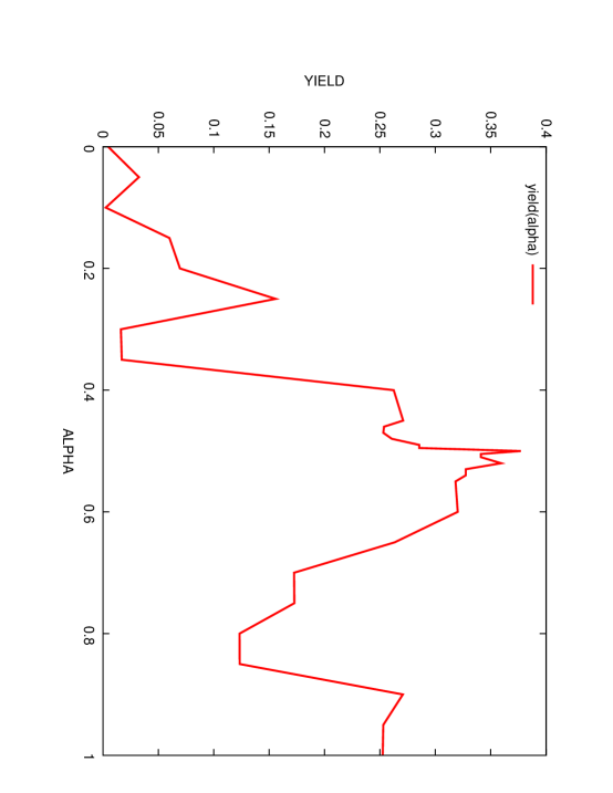
Figure 1: yield as a function of alpha

7.2.1 Additional tests

The next set of experiments address basic conjectures that arise in the context of the type of control that we consider:

• It is best to stop the cascade in the first round, i.e. to sufficiently reduce demands in the first round so as to eliminate all line overloads.

• It is best to apply control in the first round only, and ride out the cascade for the remaining rounds.

In fact it is a simple task to create small examples where both conjectures above are proved wrong. Instead we explore these questions using the Eastern Interconnect, with a random interdiction of the type described above with $K=50$, three rounds, and $\alpha=1$ (no memory, and thus we obtain outage rule (F.1)). The results of this experiments are as follows:

• Using no control, after three rounds $0.63\%$ of the demand is satisfied.

• Grid search produces a control with yield $45.46\%$.

• Starting from this control, and using segmented search with $50$ segments improves yield to $50.02\%$.

To gain a different perspective on this cascade, consider Table 10, which shows the distribution of line overloads at the start of the cascade.

Table 10: Distribution of line overloads

$\lceil$ overload $\rceil$	1505	58	48	32	22	19	11	7	6	5	4	3	2
count	1	1	2	1	2	1	1	2	2	4	6	18	181

Where $f^{1}$ denotes the flow vector at the start of the cascade, the table indicates the quantity of lines $j$ whose (rounded-up) overload $\lceil|f^{1}_{j}|/u_{j}\rceil$ equals a particular value. Thus, $181$ lines $j$ are such that $1<|f^{1}_{j}|/u_{j}\leq 2$, $18$ lines $j$ are such that $2<|f^{1}_{j}|/u_{j}\leq 3$, and so on. One line has overload greater than $1504.93$. We will provide a more detailed analysis of this case in the near future; however it is the case (as may seem plausible from the table) that in order to stop all overloads in round 1 a drastic reduction of demands is needed. We will instead describe the behavior of the optimal control computed by grid search has $(c^{1}_{v},b^{1}_{v},s^{1}_{v})=(300.7,1,0.0004)$, and $(c^{2}_{v},b^{2}_{v},s^{2}_{v})=(1.26,1,0.62)$.

Thus, in round 1, all demands will be scaled by a (approximately) factor of $1.0+0.0004*(300.7-1504.93)=0.51831$. Considering Table 10, we see that in round 1 all lines included in the columns with overload greater than $2$ will be outaged – this is a total of $41$ lines, and in fact three more with overload close to $2$ are outaged.

At the start of round 2, the maximum overload is approximately $1.36194$. Thus, the control specifies that demands will be reduced by a factor of $1.0+0.62*(1.26-1.36194)=0.9368$. This does not completely remove all overloads and an additional $4$ lines become outaged.

Finally, at the start of round 3, the maximum overload is $1.067891$. By the rules of our cascade model, this overload is now removed by scaling down all demands. Altogether, we obtain a yield of $0.51831*0.9368/1.067891=0.4547$, as stated above.

8 Stochastic optimization

To further motivate the need for stochastic modeling, we consider the same setup as for the experiment in Figure 1: $R=8$, $K=50$ and $\alpha=0.5$. We simulated the behavior of the computed control using the stochastic outage rule (5)-(7), repeated here for convenience. We are given a parameter $0<\epsilon<1$; if $\tilde{f}$ is a flow vector, then line $j$ is not outaged if $|\tilde{f}_{j}|<(1-\epsilon)u_{j}$, it is outaged if if $|\tilde{f}_{j}|>u_{j}$, and is outaged with probability $1/2$ if $(1-\epsilon)u_{j}\leq\tilde{f}_{j}\leq u_{j}$.

For various values of the tolerance $\epsilon$, we simulated the cascade $10000$ times. For $\epsilon<0.03$ little difference was observed with the nominal (deterministic) setting in that the average yield was close to (the deterministic yield of) $50\%$. For $\epsilon=0.03,0.10$ and $0.20$ the results are displayed in Figure 2.

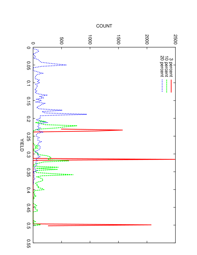
Figure 2: yield histogram under stochastic outages

The figure shows, for each value of the yield (and for each of the three choices for $\epsilon$) how frequently that yield was observed. Note that for $\epsilon=0.03$ the distribution is essentially trimodal. This is typical behavior and it points to a small number of critical lines, which, in turn, result in a small number of cascade trajectories being overwhelmingly likely. For $\epsilon=0.20$ yields close to zero are observed, but, significantly, the average is positive.

In a stochastic setting, the yield $\Theta^{R}(c,b,s)$ resulting from a control $(c,b,s)$ is a random variable. Below we discuss different methodologies for computing a (locally) optimal stochastic control, with the objective of maximizing the expectation $\rm E(\Theta^{R})$. Other merit criteria are also of interest (and possibly better), such as a linear combination of expectation and variance $\rm E(\Theta^{R})-\lambda\,var(\Theta^{R})$ ($\lambda\geq 0$), or a Sharpe-ratio quantity $\rm E(\Theta^{R})/var(\Theta^{R})$.

The computational challenges inherent in any of these tasks are significant. First, as displayed in Figure 2, yield variances can be extremely large. From a theoretical perspective, the number of samples needed to obtain reliable estimates become inordinately large. Additionally, there are subtle difficulties due to the non-monotonic behavior of power flow systems (see [6]), which is reminiscent of Braess’ paradox [8].

An example of this behavior is provide by our stochastic outage rule (3.2). Note that under this rule, a line is more likely to become outaged than under the deterministic rule (i.e., when $(1-\epsilon_{r})u_{j}<\tilde{f}^{r}_{j}\leq u_{j}$ the line may become outaged in the stochastic setting; not so in the deterministic setting). Nevertheless, one can produce cases where the deterministic yield of a control is smaller than a sample yield of the same control under rule 3.2. This phenomenon slows down convergence of our algorithms and makes algorithm calibration difficult.

8.1 Optimization methods through simulation

In either the first-order procedure (6.1) discussed above, or in the grid-search setting, we obtain a counterpart valid for a stochastic setting by replacing each (deterministic) evaluation of a yield $\Theta^{R}(c,b,s)$ by an estimation of $\rm E~{}\Theta^{R}(c,b,s)$.

This is the approach used in the next set of experiments, which parallel those in Section 5. For convenience, we restate the setup for these tests.

First, two random, though adversarially chosen lines were removed from the grid. Next, we compute the best control such that

• $c^{r}_{v}=b^{r}_{v}=1$ for all $v$ and $r$.

• $s^{r}_{v}=0$ for all $v$ and $10<r$. Thus, no control is applied after round 10.

• For each $1\leq r\leq 10$, either $s^{r}_{v}=0.005$ for all $v$, or $s^{r}_{v}=0$ for all $v$.

This was done, in the deterministic setting, while setting the maximum number of rounds, $R$, to $10$, $15$ $20$ and $25$. In Section 5, we observed that the cascade is characterized by high line overloads during the initial rounds; nevertheless if “enough” rounds are allowed ($34$) then without control the cascade stabilizes and produces approximately $78\%$ yield, and this was slightly superior to what was obtained by the controls we computed. In summary, this case provides a good contrast between the (opposing) need to “wait out” an initially severe cascade on the one hand, with uncertainty growth as we increase the number of rounds. Using the framework of stochastic outage rule (3.2), with

$$\epsilon_{r} = 0.01\,+0.05*\lfloor r/10\rfloor,$$ (24)

we observed that the (deterministic) $20$-round control appeared superior.

In this section we will repeat these comparisons, except that now we will compute controls of the form (i)-(iii) that (approximately) maximize the expected yield. We compute such controls by modifying our grid search: we evaluate a control vector by simulating $20$ cascades and computing the sample average yield. This can be a somewhat coarse approximation because, depending on the model for noise, many more than $20$ samples may be needed for an accurate answer since the variance of yield can be high.

Table 11: Stochastic grid search results in case from Section 5

R	ave kR	std kR	ave kR	std kR	ave cR	std cR
	N = 20	N = 20	N = 1000	N = 1000	N = 1000	N = 1000
20	55.78	11.88	50.23	18.57	41.90	27.47
15	48.85	10.03	41.32	13.43	33.94	22.51
10	37.16	10.74	28.65	15.13	7.54	9.55

For $R=10,15,20$, denote by kR the control computed by the algorithm. Table 11 shows the results of our experiments. In the table, for each $R$, ’ave kR’ and ’std kR’ are the estimates of the average and standard of the yield of kR using $N=20$ and $N=1000$ samples. Finally, ’ave cR’ and ’std cR’ are the 1000-sample average and standard deviation of yield of the deterministic controls c20, c15, c10, computed in Section 5 (as in Table 4).

We see that the kR controls are uniformly superior to their cR counterparts, sometimes by almost one standard deviation. We observe that k20 is superior to k15, and much superior to k10. This parallels observations made in Section 5.

8.2 Stochastic gradients

The stochastic gradients method is a well-known approach for solving optimization problems with uncertainty. Because of the nonconcave nature of the yield maximization problem, in our case it will amount to a local search method. Furthermore, there are some difficulties that are caused by the nonsmoothness in our models. We will only outline here how we are approaching these difficulties.

The core step in the stochastic gradients approach is to (randomly) sample a cascade, and, keeping the cascade fixed, to compute the impact on yield of infinitesimally small changes in the control parameters. This is followed by a line search to optimize the step size. This basic step is repeated.

A difficulty that we encounter when we attempt to make this outline more specific is that yield is not a differentiable function of the control parameters, for several reasons, the main one being the stochastic outage protocol (3.2), which, while smoother than a completely deterministic rule, is not smooth enough, due to its abrupt transition between stochastic and deterministic regimes.

We modify rule (3.2) so that the probability of a line will outage is always strictly positive and strictly smaller than $1$; however when the overload is larger than $1$ the outaging probability will be very close to $1$, and when the overload is significantly less than $1$ the outaging probability (while positive) will be very small. To this effect consider a function

$$F\,:\,\mathbb{R}_{+}\,\rightarrow\,[0,1),\ \ \ \mbox{with}\ \ F(0)=0\ \mbox{and}\ F(x)\rightarrow 1\ \ \mbox{as}\ \ x\rightarrow+\infty,$$

where the convergence is very rapid. An example is $F(x)\,=\,1-e^{-Mx}$, for large $M>0$. Likewise, consider a function

$$G\,:\,[0,1]\,\rightarrow\,[0,1),\ \ \ \mbox{with}\ \ G(0)=1\ \mbox{and}\ G(x)\rightarrow 0\ \ \mbox{as}\ \ x\rightarrow 1,$$

and again with rapid convergence. An example is $G(x)\,=\,e^{-Mx}$ for large $M>0$.

Having chosen $F$ and $G$, we modify outage rule (3.2) as follows. At round $r$, and given a tolerance $0\geq\epsilon_{r}<1$, line $j$ is outaged

with probability $$\left\{\begin{array}[]{lll}\frac{1}{2}G\left(1-\tilde{f}^{r}_{j}/(1-\epsilon_{r})\right),&\mbox{if $\tilde{f}^{r}_{j}\leq(1-\epsilon_{r})u_{j}$}&\\ &&\\ \frac{1}{2},&\mbox{if}\ {(1-\epsilon_{r})u_{j}<\tilde{f}^{r}_{j}<u_{j}}&\\ &&\\ \frac{1}{2}\left(1+F\left(\tilde{f}^{r}_{j}/u_{j}\ -\ 1\right)\right),&\mbox{if $u_{j}\leq\tilde{f}^{r}_{j}$}.&\\ \end{array}\right.$$ (30)

In other words, if $\tilde{f}^{r}_{j}>u_{j}$, the outage probability is very large, but is bounded strictly away from $1$, and if $\tilde{f}^{r}_{j}<(1-\epsilon_{r})u_{j}$ the outage probability is very small but remains strictly positive. By choosing $F$ and $G$ appropriately we obtain an outage model that is arbitrarily close to rule (3.2).

Another source of nonsmoothness in our models is the general form our control law in Step 2 of Procedure (4.2). However, it is easy to see that the law can be approximated (arbitrarily closely) using a smooth control.

The computation of the (stochastic) gradient of the yield function at a given control vector $(\bar{c},\bar{b},\bar{s})$ can now be described. First, we sample a random cascade under the control $(\bar{c},\bar{b},\bar{s})$ and outaging lines using rule (30). This produces a particular sequence of lines that become outaged; i.e. at round $r$ a certain set $S^{r}$ of lines is outaged, for $r=1,2,\ldots,R-1$.

Next, we compute the change in yield that results when we perturb the control by a vector $(\epsilon^{c},\epsilon^{b},\epsilon^{s})$ with infinitesimally small entries, while still assuming that set $S^{r}$ is the set of lines outaged at round $r$, for each $r$. This is a deterministic computation; rule (30) guarantees that the given cascade structure retains positive probability. This computation gives us the stochastic gradient.

However, at this point we need to deal with the final reason that the yield function is not smooth, and this is the demand/supply adjustment in Step 3 of our generic cascade template (3.1) (or in Step 6 of the cascade control template (4.1)). If, at round $r$, under control $(c,b,s)$ a certain component $K$ has equal demand and supply, then no adjustment takes place. However, even a small change in the control that results in shedding less demand by round $r$ will not result in an increase of yield, whereas the opposite change in control will possibly result in a decrease in yield. Thus, in essence, a left derivative is different from the right derivative; and moreover this is not a probability zero event.

Nevertheless, it is still possible to adjust the stochastic gradients framework so as to recover a valid first-order method. The resulting approach is related to the classical Frank-Wolfe method [3]. In forthcoming work we will report on experiments with this approach.

9 Upcoming work

Our forthcoming work will focus on three areas: stochastics or robustness, in particular concerning the optimal scaling problem in Section 6.2, an investigation of game-theoretic aspects of the type of control we study, and the use of AC power flow models.

With regards to the last point, a recent paper of Lavaei and Low [20] may yield a robust solver for AC power flow systems under severe contingencies. Even though the work in [20] relies on semi-definite programming, in fact one of the algorithms can be restated as a second-order conic program, which may be more efficient.

Appendix A Appendix - Formulations for the Optimal Demand Shedding Problem

We will first describe mixed-integer programming formulation for computing an optimal schedule for demand shedding, under deterministic line outages. In the formulation below our variables have the following interpretations:

• $f^{r}_{j}$ is the flow on line $(j)$ during round $r$ and $\pi^{r}_{j}$ ($\nu^{r}_{j}$) is the positive (resp., negative) part of $f^{r}_{j}$

• $\phi^{r}_{i}$ is the phase of bus $i$ during round $r$

• for a demand bus $i$, $d^{r}_{i}$ indicates its demand during round $r$

• for a generator bus $i$, $s^{r}_{i}$ indicates its supply during round $r$

• for a line $j$, the variable $y^{r}_{j}$ takes value $1$ if arc $j$ becomes outaged during round $r$ (and it takes value $0$ otherwise).

• for a line $j$, the $0/1$ variable $p^{r}_{j}$ takes value $1$ if $f^{r}_{j}>0$; likewise $n^{r}_{j}$ takes value $1$ if $f^{r}_{j}<0$

For a demand bus $i$, we indicate by the constant $\tilde{d}_{i}$ its demand at the start of the cascade. Let $\tilde{D}$ denote the sum of all such quantities $\tilde{d}_{i}$. The formulation is as follows:

$$\max\sum_{i\in{\cal D}}d^{R}_{i}$$

Subject to: $$\sum_{j\in\delta^{+}(i)}f^{r}_{j}-\sum_{j\in\delta^{-}(i)}f^{r}_{j}=\left\{\begin{array}[]{lll}~{}~{}s^{r}_{i}&{i\in{\cal G}}&\\ -d^{r}_{i}&{i\in{\cal D}}&\\ ~{}~{}0&\mbox{otherwise}&\end{array}\right.\ \forall\,1\leq r\leq R$$ (44)

$$f^{r}_{j}\,=\,\pi^{r}_{j}-\nu^{r}_{j}\,\,\,\forall\,\,j\in{\cal A}\,\,\mbox{and $1\leq r\leq R$}$$

$$\pi^{r}_{j}\,\leq\,\tilde{D}p^{r}_{j},\ \ \nu^{r}_{j}\,\leq\,\tilde{D}n^{r}_{j},\,\,\,\forall\,\,j\in{\cal A}\,\,\mbox{and $1\leq r\leq R$}$$

$$p^{r}_{j}\,+\,n^{r}_{j}\,=\,1-\sum_{h=1}^{r-1}y^{h}_{j},\,\,\,\forall\,\,j\in{\cal A}\,\,\mbox{and $1\leq r\leq R$}$$

$$\pi^{r}_{j}+\nu^{r}_{j}-u_{j}\,\leq\,\tilde{D}y^{r}_{j}\,\,\,\forall\,\,j\in{\cal A}\,\,\mbox{and $1\leq r\leq R$}$$

$$\pi^{r}_{j}+\nu^{r}_{j}\,\geq\,u_{j}y^{r}_{j}\,\,\,\forall\,\,j\in{\cal A}\,\,\mbox{and $1\leq r\leq R-1$}$$

$$\pi^{R}_{j}+\nu^{R}_{j}\,\leq\,u_{j}\,\,\,\forall\,\,j\in{\cal A}$$

$$|\phi^{r}_{i}-\phi^{r}_{j}-x_{j}f^{r}_{j}|\,\leq\,M_{j}~{}\sum_{h=1}^{r-1}y^{h}_{j}\ \ \ \forall j\in{\cal A}$$

$$0\leq s_{i}^{r}\leq\tilde{s}_{i}\,\,\,\forall\,i\in{\cal G},\ \ \ \ 0\leq d_{i}^{r}\leq\tilde{d}_{i}\,\,\,\forall\,i\in{\cal D},$$

$$p^{r}_{j},\,n^{r}_{ij},\,y^{r}_{j}\,=\,0\ \mbox{or $1$},\,\,\,\forall\,\,j\in{\cal A}\,\,\mbox{and $1\leq r\leq R$}$$

$$0\leq\pi^{r}_{j},\,0\leq\nu^{r}_{j},\,\,\,\forall\,\,j\in{\cal A}\,\,\mbox{and $1\leq r\leq R$}.$$

In this formulation, (44) is a flow balance constraint: it specifies that during round $r$ each generator $i$ outputs $s^{r}_{i}$ units of flow, and similarly with demand buses. Constraints (44)-(44) together with the fact that $p^{r}_{j}$ and $n^{r}_{j}$ are $0/1$ variables, guarantee that $\pi^{r}_{j}$ ($\nu^{r}_{j}$) is the positive (resp., negative) part of $f^{r}_{j}$, and that furthermore $f^{r}_{j}=0$ if line $j$ was outaged at a round prior to $r$. Constraint (44) guarantees that if $y^{r}_{j}=0$ then $|f^{r}_{j}|\leq u_{j}$ and (44) guarantees that if $y^{r}_{j}=1$ then $|f^{r}_{j}|\geq u_{j}$. Thus, we obtain a mix of the two alternative versions of rule (F.1).

Constraint (44) indicates the desired termination condition in round $R$. We note that (44) involves an absolute value but is easily replaced by two standard linear inequalities. The quantity $M_{j}$ is assumed to be a “large enough” quantity (see [5] for a related discussion).

Other formulations are possible, and in particular it is easy to enforce additional rules constraining how demand can be shed. The formulation can also be adapted to use the memory-dependent outage models (3) or (4). By adapting constraints (44) and (44) one can model the stochastic rule (F.2), obtaining a (mixed-integer) stochastic program; the underlying uncertainty is primarily of an endogenous nature; see [14].

A.0.1 Discussion

The above problem, even in its simplest, deterministic form is likely quite nontrivial. Constraints (44) and (44) are essential in modeling the outaging of lines; similar constraints are used in formulations for the classical $N-K$ problem (see [5], [6]) and contribute to make the problem very difficult. Note that we would need to handle cases with $n>10^{4}$, $m>2\times 10^{4}$ (and $R>2$).

A larger concern involves the fact that the optimal solution is likely to entail very complex control strategies that may be difficult to implement. All the approaches we discussed above, including the stochastic programming versions of the formulation, are likely to specify very precise actions in each round (and scenario) which may be problematic in practice in what likely would be a very “noisy” environment.

Nevertheless, the study of the formulation may still prove a very worthwhile exercise, one that could highlight underlying weaknesses of the models and hidden vulnerabilities in the operation of the grid.

References

- [1] R. K. Ahuja, T. L. Magnanti, and J. B. Orlin. Network Flows: Theory, Algorithms, and Applications. Prentice Hall, NJ (1993).
- [2] G. Andersson, Modelling and Analysis of Electric Power Systems. Lecture 227-0526-00, Power Systems Laboratory, ETH Zürich, March 2004. Download from http://www.eeh.ee.ethz.ch/uploads/tx ethstudies/modelling hs08 script 02.pdf.
- [3] D. Bertsekas, Nonlinear Programming, Athena Scientific (2003).
- [4] A. Bergen and V. Vittal, Power Systems Analysis, Prentice-Hall (1999).
- [5] D. Bienstock and S. Mattia, Using mixed-integer programming to solve power grid blackout problems, Discrete Optimization 4 (2007), 115–141.
- [6] D. Bienstock and A. Verma, The Problem in Power Grids: New Models, Formulations, and Numerical Experiments, SIAM J. Opt. 20 (2010), 2352–2380.
- [7] S. Boyd and L. Vandenberghe, Convex Optimization. Cambridge University Press.
- [8] D. Braess, Über ein Paradox der Verkerhsplannung, Unternehmenstorchung Vol. 12 (1968) 258–268.
- [9] B.A. Carreras, V.E. Lynch, I. Dobson, D.E. Newman, Critical points and transitions in an electric power transmission model for cascading failure blackouts, Chaos, vol. 12, no. 4, 2002, 985-994.
- [10] B.A. Carreras, V.E. Lynch, D.E. Newman, I. Dobson, Blackout mitigation assessment in power transmission systems, 36th Hawaii International Conference on System Sciences, Hawaii, 2003.
- [11] B.A. Carreras, V.E. Lynch, I. Dobson, D.E. Newman, Complex dynamics of blackouts in power transmission systems, Chaos, vol. 14, no. 3, September 2004, 643-652.
- [12] B.A. Carreras, D.E. Newman, I. Dobson, A.B. Poole, Evidence for self organized criticality in electric power system blackouts, IEEE Transactions on Circuits and Systems I, vol. 51, no. 9, Sept. 2004, 1733- 1740.
- [13] A.R. Conn, K. Scheinberg and L.N. Vicente, Introduction to derivative-free optimization, MPS-SIAM Series on Optimization, Philadephia (2009)
- [14] V. Goel, and I.E. Grossmann, A class of stochastic programs with decision dependent uncertainty, Mathematical Programming 108 (2006) 355-394.
- [15] Gurobi Optimization, Houston TX.
- [16] D.F. Hobbs, M.H. Rothkopf, R.P. O’Neill and H.-P. Chao (eds), The Next Generation of Electric Power Unit Commitment Models. Kluwer Academic Publishers (2001).
- [17] The IEEE reliability test system–1996, IEEE Trans. Power Syst. 14 (1999) 1010 - 1020.
- [18] IBM ILOG, Incline Village NV.
- [19] H.J. Kushner and D.S. Clark, Stochastic approximation methods for constrained and unconstrained systems. Springer-Verlag Berlin, (1978).
- [20] J. Lavaei and S. Low, Zero Duality Gap in Optimal Power Flow Problem, manuscript (2010).
- [21] J.T. Linderoth and S. J. Wright, “Decomposition Algorithms for Stochastic Programming on a Computational Grid, “ Computational Optimization and Applications Vol 24 (2003) 207–250.
- [22] D.G. Luenberger, Linear and Nonlinear Programming, Addison-Wesley (1984).
- [23] A. Pinar, J. Meza, V. Donde, and B. Lesieutre, Optimization Strategies for the Vulnerability Analysis of the Electric Power Grid, SIAM Journal on Optimization 20 (2009), 1786–1810.
- [24] H. Robbins and S. Monro, On a stochastic approximation method, Annals of Mathematical Statistics 22 (1951), 400 - 407.
- [25] Final Report on the August 14, 2003 Blackout in the United States and Canada: Causes and Recommendations, U.S.-Canada Power System Outage Task Force, April 5, 2004. Download from: https://reports.energy.gov.
- [26] A. Wächter and L. T. Biegler, On the Implementation of an Interior-Point Filter Line-Search Algorithm for Large-Scale Nonlinear Programming Mathematical Programming 106 (2006), 25 – 57.