1.2 Meter Shielded Cassegrain Antenna for Close-Packed Radio Interferometer

Abstract

Interferometric millimeter observations of the cosmic microwave background and clusters of galaxies with arcmin resolutions require antenna arrays with short spacings. Having all antennas co-mounted on a single steerable platform sets limits to the overall weight. A 25 kg lightweight novel carbon-fiber design for a 1.2 m diameter Cassegrain antenna is presented. The finite element analysis predicts excellent structural behavior under gravity, wind and thermal load. The primary and secondary mirror surfaces are aluminum coated with a thin TiO₂ top layer for protection. A low beam sidelobe level is achieved with a Gaussian feed illumination pattern with edge taper, designed based on feedhorn antenna simulations and verified in a far field beam pattern measurement. A shielding baffle reduces inter-antenna coupling to below $\sim$ -135 dB. The overall antenna efficiency, including a series of efficiency factors, is estimated to be around 60%, with major losses coming from the feed spillover and secondary blocking. With this new antenna, a detection rate of about 50 clusters per year is anticipated in a 13-element array operation.

1 Introduction

The Array for Microwave Background Anisotropy (AMiBA) is a forefront radio interferometer for research in cosmology. This project is led, designed, constructed, and operated by the Academia Sinica, Institute of Astronomy and Astrophysics (ASIAA), Taiwan, with major collaborations with National Taiwan University, Physics Department (NTUP), Electrical Engineering Department (NTUEE), and the Australian Telescope National Facility (ATNF). Contributions also came from the Carnegie Mellon University (CMU), and the National Radio Astronomy Observatory (NRAO). As a dual-channel 86-102 GHz interferometer array of up to 19 elements, AMiBA is designed to have full polarization capabilities, sampling structures on the sky greater than 2 arcmin in size. The AMiBA target science is the distribution of high red-shift clusters of galaxies via the Sunyaev-Zel’dovich Effect (SZE), e.g. Sunyaev & Zel’dovich (1972); Birkinshaw (1999); Carlstrom et al. (2002) and references therein, as a means to probe the primordial and early structure of the Universe. AMiBA will also measure the Cosmic Microwave Background (CMB), e.g. Spergel et al. (2007); Aghanim et al. (2008); Larson et al. (2010), temperature anisotropies on scales, which are sensitive to structure formation scenarios of the Universe. AMiBA is sited on Mauna Loa in Hawaii, at an elevation of 3,400m to take advantage of higher atmospheric transparency and minimum radio frequency interference.

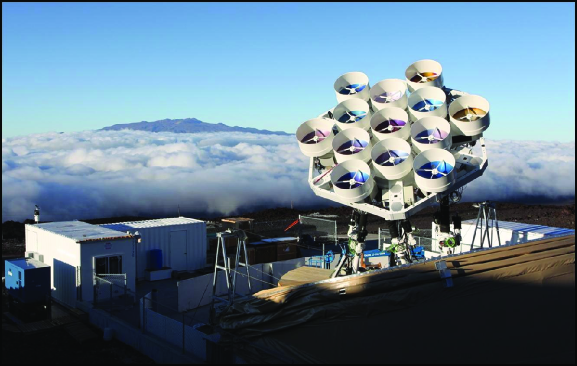
Figure 1: Front view of the AMiBA in the completed expansion phase with 13 1.2 m diameter Cassegrain antennas. All antennas are co-mounted on a fully steerable six meter carbon-fiber platform which is driven by a hexapod telescope. The antenna shielding baffles are clearly visible. Free receiver holes in the platform (covered with aluminum plates on the photo) allow for different array configurations.

After an initial phase with seven 0.6 m diameter antennas (Koch et al., 2006) in a compact configuration, the AMiBA is currently operating with 13 1.2 m diameter Cassegrain antennas (Figure 1). This new antenna and its capabilities are described here. Section 2 lists the antenna requirements. In Section 3 the mechanical and optical designs are detailed out, including simulation results of the structure and the antenna-feedhorn system. Section 4 is devoted to the antenna verification measurements. The factors composing the antenna efficiency are estimated in Section 5. Section 6 discusses the improved design features of the 1.2 m antenna and the upgraded array operation. Our conclusion is given in Section 7.

Previous AMiBA progress reports were given in Ho et al. (2004); Raffin et al. (2004); Li et al. (2006); Raffin et al. (2006). A project overview is given in Ho et al. (2009). More details about the correlator and receiver can be found in Li et al. (2010) and Chen et al. (2009). The hexapod telescope mount is introduced in Koch et al. (2009). Observing strategy, calibration scheme and data analysis with quality checks are described in Lin et al. (2009); Wu et al. (2009); Nishioka et al. (2009). First AMiBA science results from the 7-element array are presented in Huang et al. (2009); Liao et al. (2010); Koch et al. (2010); Liu et al. (2009); Umetsu et al. (2009); Wu et al. (2009). A possible science case utilizing the 1.2 m antenna array configuration is outlined in Molnar et al. (2010).

2 Antenna Requirements

Antenna size and interferometric baselines are constrained by the required window functions sampling the scales on the sky, which are relevant for our target science. After the AMiBA initial phase with seven 0.6 m diameter antennas in close-packed configuration, 13 1.2 m diameter antennas are now installed, covering a baseline range from 1.4 m to about 6 m. This gives a synthesized beam resolution of about 2 arcmin for a nominal central frequency of about 94 GHz The collecting area of the 13-element array is increased by a factor of 7.4 upon the initial phase.

The antenna pointing accuracy and its mechanical stiffness requirements against wind force, self-gravity and thermal load are driven by its field of view (FoV), which is about $11^{\prime}$ at Full Width Half Maximum (FWHM) at 94 GHz (Section 3.3 and Section 4.2). We consider deformations and mechanical alignment errors resulting in less than a $1^{\prime}$ tilt ($\sim 10$% of FWHM) as acceptable. Minimizing deformations also ensures that the asymmetrical patterns on the antenna surface and the resulting antenna cross-polarization are kept at a low level. The manufacturing accuracy of the mirror surfaces is specified to be better than $50\mu$m root-mean-square (rms) to ensure an antenna surface efficiency of more than 95% (Section 3.1 and Section 4.1).

Measuring the weak CMB fluctuations ($\sim 10\mu$K) requires a low-noise antenna with low side lobe levels and very little scattering and cross talk. High sidelobes are suppressed with a $-10.5$ dB edge taper in the feed’s Gaussian illumination pattern (Section 3.3 and Section 5). The antenna is shielded with a baffle to minimize the inter-antenna coupling and the ground pickup. Additional care is taken to send stray-light back to the sky with triangular roof-shaped quadripod legs (Section 3.4).

Due to the harsh volcanic environment together with the large high-altitude temperature variations we decided to add a TiO₂ protection layer on both the primary and secondary mirrors against abrasion. Furthermore, visual and infrared sun light is a potential hazard to burn our antennas. The 0.6 m diameter antennas were therefore additionally covered with a Gore-Tex layer on top of the shielding baffle in order to absorb the damaging radiation. At our observing microwave frequencies both the protection layer and the cover are designed to minimize the absorption loss and maximize the reflectivity and the transmission, respectively (Section 4.4). On the 1.2 m diameter antennas no Gore-Tex cover is needed because most of the visible and infrared light is not reflected by the TiO₂ coated surfaces.

Finally, minimizing any torque and possible tilting of the antennas when mounted on the receivers is crucial to reach a stable radio alignment. On top of that, in order to keep the total weight below the acceptable limits of the hexapod telescope, a lightweight structure is needed together with the desirable radio frequency properties. Choosing carbon fiber reinforced plastic (CFRP) satisfies these conditions and keeps the weight of the antenna below 25kg.

3 Mechanical and Optical Design

Section 3.1 describes the basic Cassegrain antenna design. The results from the antenna structure and antenna-feedhorn simulations are described in Sections 3.2 and 3.3. The Sections 3.4 and 3.5 discuss in more details the additional measures taken to control antenna cross-talk and to reduce ground pick-up and stray-light.

3.1 Cassegrain Antenna Geometry

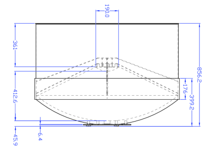
Figure 2: Drawing of the assembled antenna including the main components: primary and secondary mirror, structure and shield baffle, quadripod support legs and hexagonal bottom support plate. The units are in mm.

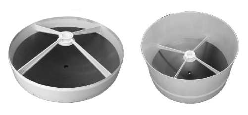
Figure 3: The AMiBA 1.2m Cassegrain antenna: on the left hand side the antenna with the structure baffle only, on the right the complete antenna with the shielding baffle. The secondary mirror quadripod leg support is attached to the structure baffle.

Based on requirements (Section 2), a shielded f/0.35 Cassegrain antenna was chosen. Tables 1 and 2 present the specifications for the primary paraboloid and the secondary hyperboloid mirrors. The Figures 2 and 3 show a drawing and a picture of the assembled antenna, respectively.

The Cassegrain geometry sets the feed phase center at the vertex of the primary. A parabolic illumination grading leads to about -20 dB for the first side lobe and a 11^′ FWHM for the primary beam at a wavelength of $\lambda\sim 3.2$ mm ($\sim$ 94 GHz). Sub-reflector and feed positioning requirements are based on the Ruze formulas (Ruze, 1966). An axial and lateral secondary defocus of 0.1 $\lambda$ and 0.45 $\lambda$, respectively, keeps the gain loss at less than 1 %. Similarly, a feed horn positioning within 1 $\lambda$ gives a 99 % gain. Random surface deviations from a primary paraboloid and a secondary hyperboloid will remove power from the main beam and distribute it in a scattered beam. A surface error of less than 50 $\mu$m rms from the ideal geometry ensures a 95% gain.

3.2 Structure Simulations

Typical load cases on the AMiBA site include wind, low temperatures and gravity load. Based on stiffness requirements and weight considerations, carbon fiber reinforced plastic (CFRP) was chosen for the dish, the feedlegs and the baffle. The primary and secondary mirrors are sandwich composites. The baffle is made of two parts (Figure 2): a structural baffle supporting the feed-legs and a non-structural (shielding) baffle fixed to the latter to prevent cross-talk between antennas and minimize ground pick-up. Mass is an issue as the AMiBA platform is designed to accommodate up to 19 identical antennas, but the hexapod drive systems sets an overall weight limit. From an original 50 kg prototype antenna, the weight was reduced to about 25 kg with the help of a Finite Element Analysis (FEA), while maintaining the overall structural behavior of the antenna. The main goal of the structural analysis is to ensure that the parabolic characteristics of the primary mirror are met for a minimized mass.

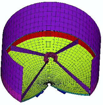
Figure 4: Grid for the FEA antenna model. 15,400 nodes and 18,300 elements are used for the structure simulation. The main components of the antenna are shown in different colors.

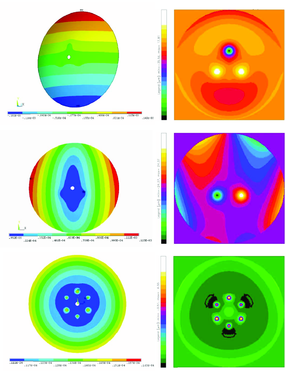
Figure 5: Selected load cases from structure simulations. The left panels display the deformation of the primary mirror. The units on the color bars are in $\mu$m. The corresponding residual maps from a best-fit paraboloid to the deformed surfaces are shown in the right panels. The units are in $\mu$m. The top panels illustrate the deformation due to gravity load along the $y$-axis at an elevation of 30 deg. The maximum peak-to-peak (PTP) deformation is 0.3 mm (right panel), which leads to a 53 $\mu$m PTP and 4 $\mu$m rms deviation from a best-fit paraboloid (left panel). A 10 m/s side wind load at $el=90$ deg is analyzed in the middle panels. The primary mirror maximum PTP normal deflection is 0.115 mm. Residual maximum PTP and rms deviations are 49 $\mu$m and 5 $\mu$m, respectively. A uniform temperature increase of 20^∘C is simulated in the bottom panels, leading to maximum normal deflections of 5 $\mu$m, and a residual maximum PTP and rms deviation of 5 $\mu$m and 1 $\mu$m, respectively.

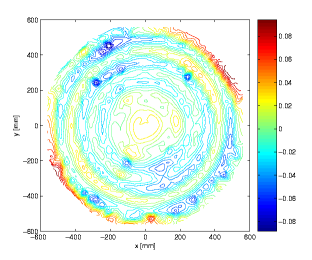
Figure 11: Contour plot of the fitting residuals from a a best-fit parabolic primary mirror. The units are in mm. The surface accuracy is about 28 $\mu$m rms, with maximum deviations of 96 $\mu$m and -98 $\mu$m, respectively, leading to a focal distance $F_{p}=413.66$ mm. The systematic ring-like pattern in the residuals reveal an imperfect manufacturing process (likely resulting from an uneven support during the machining) at a level which is irrelevant for our frequency range around 94 GHz.

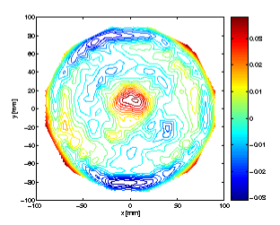
Figure 12: Contour plot of the fitting residuals from a a best-fit hyperbolic secondary mirror. The units are in mm. The surface accuracy is about 13 $\mu$m rms, with maximum deviations of 42 $\mu$m and -34 $\mu$m, respectively, leading to a focal distance $F_{p}=413.59$ mm.

The simulation results presented in this section refer to the production antenna. Figure 4 shows the grid of the FEA model. The finite element model was analyzed with ANSYS version 11 with 15,400 nodes and 18,300 elements. In particular, 3D-Shell elements were used to model the CFRP primary mirror skins, the baffle and feed-legs, and the sub-reflector coupling. 3D-Solid elements were adopted to model the core of the primary mirror, the structural baffle and the hexagonal support plate sandwich composites. Finally, 3D-Beam uniaxial elements served to model the sub-reflector and the inserts. Boundary conditions apply on the hexagonal support plate and are not symmetrical with respect to the antenna geometry. Therefore, structural behavior varies with the antenna orientation in its aperture plane. For each individual load case (gravity, wind load and thermal load) the deformation (Figure 5, left panels) is calculated from a displacement vector which is the sum of the nodal components. The residual map from a best fit paraboloid to the deformed primary mirror is shown in the right panels in Figure 5. Table 3 summarizes the results. For combined load cases the added surface deformations are within about 5 $\mu$m over the entire elevation range. This only adds insignificantly to the manufacturing random errors ($\epsilon_{\|}<30\mu$m, Section 5 and Figures 11 and 12) and, therefore, does not further reduce the efficiency. Combined resulting tilts of the optical axis are within 1 arcmin, which is at the acceptable 10% level of the FWHM ($\sim 11$ arcmin) around the operating frequency of 94 GHz. This is comparable to the achievable mechanical alignment between individual antennas on the platform which then keeps the loss in amplitude for each antenna pair at the percent level.

3.3 Feedhorn - Antenna Simulations

We designed a corrugated feedhorn with a variable-depth mode converter to cover a full 20 GHz band from 85 to 105 GHz (Zhang, 1993; Granet & James, 2005). The center frequency is around 95 GHz. The geometry of the horn is shown in Figure 6. The feedhorn has a semi-flare illumination angle of 14^∘ with a parabolic illumination grading with a -10.5 dB edge taper. Free-space tapering for f/0.35 is about 3.6 dB, which leads to about -20 dB for the first side lobe and a 11^′ FWHM for the primary beam at a wavelength of $\lambda=3.2$ mm. The analysis of the horn is done using the well-proven mode-matching technique (James, 1981). The resulting theoretical radiation pattern is shown in Figure 7. An aperture flange with an external radius of $11.86$ mm is used in the calculations. The phase-center of the horn is located 19 mm inside the horn, when measured from the aperture. The aperture of the horn is therefore located 19 mm above the vertex of the primary mirror.

The radiation pattern of the antenna has been simulated (James et al., 2000), using the following two assumptions: No feed-leg blockage and no baffle is taken into account. The radiation pattern of the horn, calculated using the mode-matching method, is then used to excite currents on the secondary mirror and the Physical Optics (PO) method is used to calculate the currents generated by the secondary onto the primary mirror. The radiation pattern of the antenna is then calculated using the combination of the contributions of the radiated power by the primary, secondary mirror and the feed (James et al., 2000).

The gain of the antenna is normalized by the input power of the horn, i.e., the return loss of the horn is included in the gain calculation. The efficiency calculation is based on a comparison between the gain of the antenna and the gain of an unblocked 1.2m-diameter with a constant amplitude and phase distribution. The radiation pattern at $95$ GHz is shown in Figure 8 while the gain of the antenna over the $85-105$ GHz band and the associated antenna efficiency are given in Table 4.

3.4 Shielding Baffle

Having several antennas in a close-packed configuration on the platform can cause cross-talk problems which might affect CMB measurements (Padin et al., 2000). The total cross-talk signal $C_{tot}$ for a single antenna is expected to be proportional to the number of neighboring antennas. This leads to a maximum cross-talk signal $C_{tot}\sim 6C$ for the central antenna in a hexagonal compact configuration (Figure 1), where $C$ is the coupling strength on the shortest baseline. The cluster SZE signal is typically about 1 mK. The CMB temperature fluctuations are $\sim 0.1$ mK on cluster scales and they decrease to $\sim 10~{}\mu$K or less on smaller scales. In comparison, the maximum false signal due to cross-talk is $T_{r}\sqrt{pC}$, where $T_{r}$ is the receiver noise and $p$ is the correlation coefficient between the outgoing and receiver noises (Thompson & D’Addario, 1982; Padin et al., 2000). Assuming $p=0.01$ and $T_{r}=65$ K for AMiBA (Chen et al., 2009), a maximum wrong signal of $\sim 40\sqrt{C}$ K might be present at the central antenna. Adopting a 10% tolerance of the weak CMB signal, 1 $\mu$K, $C$ should be reduced to about -127 dB.

Therefore, in order to assure a low inter-antenna cross-talk, it was decided to add a shielding baffle similar to the case of the Cosmic Background Imager (CBI). Baffle height and baffle rim curvature are the important parameters to determine. Our design is closely following the antennas built for the CBI (Padin et al., 2000). Generally, the approach is to eliminate sharp discontinuities which would diffract energy from the main lobe. Therefore, scattering from the baffle shield rim is minimized by rolling the rim with a radius $\sim 5\lambda\approx 15$ mm (Mather, 1981).

Finally, when using a shielding baffle, its effect on the forward gain of the antenna needs to be considered. As an approximation in the antenna near-field, the Fresnel diffraction integral for a circular aperture is adopted to calculate the propagating electric field, $E(x,y,z)$, above the aperture plane. The aperture field distribution, $E(x,y,0)$, is a Gaussian with a -10.5 dB edge taper as a result of our feedhorn illumination. Evaluating $E$ in the center and at the radius of the baffle location as a function of distance from the aperture plane shows a close to constant ratio between them. This finding is consistent with the expected beam broadening, $w(z)=w_{0}\sqrt{1+(\frac{\lambda z}{\pi w_{0}^{2}})^{2}}$, along the optical axis, which is less than 0.1% up to a height $z=1$ m for an initial beam waist $w_{0}\approx 0.545$ m (for a Gaussian with a -10.5 dB edge taper). Consequently, the power $P\sim E^{2}$ remains well confined with a plane integrated loss of less than 1% (at a height of 1 m) compared to a broadened beam without baffle. The loss in forward gain does therefore not set any stringent constraint in this case due to the well collimated beam. Eventually, it was decided to limit the baffle height to where the tangential plane at the edge of the secondary intercepts with the baffle. In the optical geometrical limit, rays scattered from the secondary are confined to this plane. This results in a total baffle height of about $630$ mm above the aperture plane, which leaves the secondary and feedlegs about $360$ mm inside the baffle (Figure 2).

3.5 Secondary Mirror Feed Legs

Besides minimizing the antenna cross-talk, in order to further control the antenna sidelobe levels and scatter stray-light back towards the sky, the geometrical shape of the secondary mirror feed legs has been optimized. Mainly two concerns are related to the feed leg shape: the antenna sidelobe level can increase due to diffraction from the legs and the system temperature can increase due to reflected ground pickup. Satoh (1984); Moreira et al. (1996) and Lawrence et al. (1994) have extensively studied the issue of ground spillover pickup and feed leg shaping or baffling. One shaping technique is to attach a triangular roof on the lower side of the feed leg (Lamb, 1998). An optimized angle has been worked out for our Cassegrain geometry in order to keep scattered rays close to the pointing axis towards the cold sky and away from the secondary and primary mirrors. Using geometrical optics, the scattered rays are found to be within a cone with opening angle $\theta$ (Cheng & Mangum, 1998):

$$\theta=\pi/2-2\arcsin(\sin(\beta)\sin(\alpha)),$$ (1)

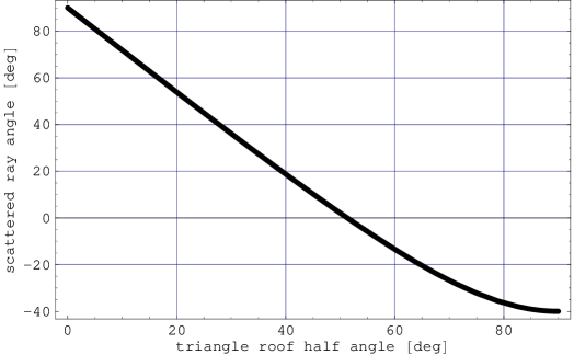
Figure 10: Scattered ray angle ($\theta$) as a function of the triangular roof half angle ($\alpha$). The scattering angle is measured with respect to the aperture plane. A positive angle means scattering towards the sky, negative angle means scattering down towards the primary mirror. A triangular roof half angle of about $15^{\circ}$ was chosen.

where $\alpha$ is the half angle of the triangular roof and $\beta$ is the angle between the lower side of the feedleg and the optical axis of the antenna. For our design, $\beta=65^{\circ}$, which is close to half of the primary mirror illumination angle because the feedlegs are attached close to the rim of the primary mirror (Figure 2). With this resulting scattering angle ($\theta$), stray-light is terminated to the cold sky. The angle $\theta$ is also well matched with the baffle height in order to avoid multiple scatterings from the baffle, which might occur if $\theta$ is too small and therefore intercepting with the upper parts of the shielding baffle. Since the height of the triangular roof increases with smaller $\alpha$, $\alpha\rightarrow 0^{\circ}$ - which would ideally send scattered rays straight to the sky ($\theta\rightarrow 90^{\circ}$) - is practically not feasible. Therefore, as a compromise $\alpha\approx 15^{\circ}$ was chosen, which confines scattered rays to within $\theta\approx 65^{\circ}$ (Figure 10) and keeps the height of the equilateral roof shape within about 20 mm. The 2-dimensional antenna beam pattern measurement in section 4.2 possibly demonstrates an improvement due to this triangular roof shape. Whereas for larger antennas an optimized leg design was able to reduce the system temperature of up to 10 K, in the case of our small antennas this might eventually be more a measure of precaution.

4 Antenna Verification

4.1 Surface and Alignment Measurements

The mirror surfaces are measured at the Center for Measurement Standards (CMS), founded by the Industrial Technology Research Institute (ITRI) in Taichung, Taiwan, using a ZEISS PRISMO 10 measuring machine with a 4.4 $\mu m$ measurement accuracy. The surfaces are checked from a sample of data points: 885 and 276 uniformly distributed points are measured across the primary and secondary mirrors, respectively. This yields sets of $(x,y,z)$-coordinates for a two-dimensional fit for the primary paraboloid and the secondary hyperboloid, respectively, using the following formula:

$$primary: z =\frac{x^{2}+y^{2}}{4F_{p}}+C_{p}$$ (2)

$$secondary: z =\sqrt{a^{2}+\frac{a^{2}}{b^{2}}(x^{2}+y^{2})}+C_{s},$$ (3)

where $F_{p}$ is the focal distance, and $C_{p}$ and $C_{s}$ are off-sets in the $z$-direction due to the measurement set-up. $a$ and $b$ determine the curvature of the hyperboloid with a resulting focal distance $F_{p}=2\sqrt{a^{2}+b^{2}}$ (Table 1 and 2). The primary and secondary mirrors typically have surface rms errors of about 30 $\mu m$ and 15 $\mu m$, respectively, as illustrated for one antenna in the Figures 11 and 12. The resulting focal length $F_{p}$ is found to be within $0.1$ mm of the specifications. This reduces the dish surface efficiency by less than 2%. After verification of the surface, the antenna is assembled and the secondary mirror is mechanically shimmed to meet the alignment criteria. The alignment is typically between $50\,\mu m$ and $100\,\mu m$ in the $x$, $y$ and $z$ translation directions. The aperture efficiency (Section 5) is therefore reduced by only less than 1%.

4.2 Antenna Beam Pattern

For precision cosmology an accurately measured antenna beam pattern is essential. The beam convolution effect reduces the information of the observed signal on small angular scales which is of particular importance for the CMB power in the multipole space. Furthermore, defects in the beam pattern, such as an increase in the side lobes or a circular asymmetry, can affect the sensitivity limits (Wu et al., 2001). Besides confirming the theoretical expectations, the detailed measurement and characterization of the antenna beam pattern makes it possible to use the exact beam response in the later science data analysis if this should be needed.

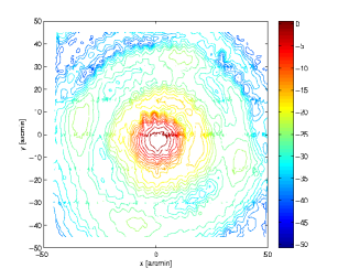
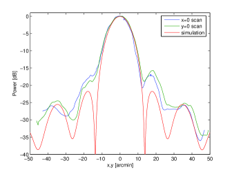
Figure 13: Left Panel: Contour plot of the antenna beam pattern measured in the far. The units are in dB. The cross-structure around the secondary sidelobes is likely to result from scattering of the secondary mirror support structure. Right Panel: One-dimensional scans, extracted from the Left Panel, parallel to the $x$- and $y$-axis after location of the main beam maximum. Overlaid is the simulation result (section 3.3) for the E-plane at 95 GHz.

We measured the beam pattern with a computer-controlled equatorial mount, scanning a fixed 90 GHz thermally stabilized CW source at a distance of about $250-300$ m. This is marginally in the far field ($\sim D_{p}^{2}/\lambda\sim 480$ m). An example of a measured beam pattern from a 2-dimensional scan is shown in the Left Panel in Figure 13. A cross-like feature likely resulting from the four legs of the secondary mirror support structure becomes apparent, with an increase in power of $\sim 1$ dB at the location of the second sidelobe. Comparing to the initial 0.6 m diameter antennas (Koch et al., 2006) - where a cross-like structure of a few dB was measured - the feature has been reduced, possibly with the help of the additional triangular roof at the secondary support structure (section 3.4). The Right Panel in Figure 13 compares two orthogonal scans across the main beam center with the expected simulation result from section 3.3 for the E-plane at 95 GHz. Whereas the measured mainlobe nicely confirms the simulation result, the first sidelobe is about $2-4$ dB higher than expected. The detailed cause of this is unclear. One might speculate that this is due to a weaker feed illumination edge taper than predicted and remaining stray light from the secondary mirror support. The location and the level of the second sidelobe agree again well with the simulation. From the measurement, a FWHM of about 11 arcmin is found with a first sidelobe peaking at about $-16$ to $-18$ dB.

The results are further analyzed following Wu et al. (2001), investigating azimuthally averaged beam profiles and $\omega_{l}$, the indices of asymmetry: $\omega_{l}=(<|B_{lm}|^{2}>-<B_{lm}>^{2})/<|B_{lm}|^{2}>$ . $B_{lm}$ is the beam multipole expansion, $l$ being related to the corresponding angular scale. $<|B_{lm}|^{2}>$ and $<B_{lm}>^{2}$ are the mean of squares over $m$ and the square of the mean over $m$, respectively. The above defined numerator is thus the variance of $B_{lm}$ about its mean over $m$, a perfectly symmetric beam giving $\omega_{l}=0$. Calculating the indices of asymmetry further requires the beam data to be pixelized. As a result, the index of asymmetry is always below 0.2 within the FWHM, indicating a good symmetry of the antennas.

4.3 Antenna Cross-Talk

Low cross-talk signals were verified on the operating 13-element array on the AMiBA site. As a measurement set-up, one antenna served as an emitter and was outfitted with a $\sim$ 10 dBm narrow-band polarized source (Gunn oscillator with a bandwidth of $\sim$ 2-3 MHz at the measured intermediate frequency (IF) of $\sim$ 5.56 GHz ). In different adjacent antennas (dual linear polarization receivers) the weak cross-talk signal was then detected with a spectrum analyzer connected to the output at the end of the first section in the IF chain. Various amplifiers along the IF chain (from the receiving feedhorn to the end of the first section) give rise to a gain of about 70 dB (Chen et al., 2009; Li et al., 2010). Subtracting that and taking into account the source power, the original cross-talk signal scattered into the feedhorn is derived.

The coupling between two 1.2 m antennas was measured for a 1.4 m and a 2.8 m baseline. In order to quantify the influence of the shielding baffle (Figure 3), the measurement was done with and without baffle. Figure 9 summarizes the results. For comparison, the smaller 60 cm antennas were also checked on a few baselines. By varying the source orientation, cross-talk signals for maximally and minimally aligned polarizations were detected. For the 1.2 m antennas without baffle, there is about a 20 dB difference on the shortest baseline depending on polarization. Generally, this difference is reduced for longer baselines, and it becomes indistinguishable on a 1.4 m baseline for the 60 cm antennas. When adding the shielding baffle, only a minor difference in polarization of $\sim$ 5 dB is found on the shortest baseline for the 1.2 m antennas. The shielding baffle reduces significantly the maximum cross-talk signal from about -115 dB to $\sim$ -135 dB or less on the 1.4 m baseline, and from $\sim$ -130 dB to $\sim$ -145 dB or less on the 2.8 m baseline. As expected, for both the 60 cm and 1.2 m antennas, the cross-talk signal rapidly decreases with distance. Thus, primarily the shortest baseline is of a concern. Here, the shielding baffle successfully reduces the cross-talk below the targeted -127 dB level. For baselines beyond 2.8 m any remaining coupling is beyond our detection limit of about -145 dB.

4.4 Material Properties

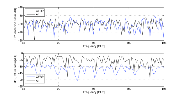
Figure 14: VNA measurement: Upper Panel: Insertion loss (S21) for both CFRP and aluminum over the frequency range $85-105$ GHz. Lower Panel: Return loss (S11).

Both the antenna structure and shielding baffle are made of carbon fiber reinforced plastic (CFRP). The material has been measured with a vector network analyzer (VNA). For a $0.72$ mm thick CFRP test sample an insertion (through put) loss (S21 parameter) of about $-62$ dB or less is measured in the frequency range of $85-105$ GHz, which is comparable to the $0.88$ mm aluminum sample which shows an insertion loss around $-60$ dB (Figure 14, Upper Panel). The values are upper limits because they are at the noise level of the VNA. The return loss (S11 parameter) averages around $-11$ dB in the observed frequency range compared to about $-5$ dB for the aluminum sample (Figure 14, Lower Panel). From this we conclude that very little radiation goes through the baffle and the deficiency in return loss (reflection) is absorbed in the material, which makes CFRP and ideal and lightweight shielding material. Similar VNA tests have also shown that a possible Gore-Tex cover to protect the antenna additionally against visible and UV-light has a transmission loss of less than $0.1$ dB.

The surface top layers of the primary and secondary mirrors are aluminum coated in the vacuum. The reflectivity of aluminum is close to 100% as soon as there are only a few layers of atoms. Further aiming at minimizing a possible emission from the underlying material, an aluminum layer attenuation to at least 1% is targeted. A 5 times skin depth leads to a reduction in amplitude by a factor of $(1/e)^{5}=0.67$%. This sets the coating layer to $\delta=5\times\sqrt{2/(2\pi\nu\mu_{0}\sigma)}\approx$ 1.4 $\mu m$ at a frequency of $\nu=$ 94 GHz. $\sigma$ and $\mu_{0}$ are the electrical conductivity for aluminum and the free space magnetic permeability, respectively. ($\sigma\approx 3.6\times 10^{7}\Omega^{-1}$m^-1 and $\mu_{0}=1.2566\times 10^{-6}$Vs/Am.) The typical aluminum layer - measured at various positions across the primary mirror - is about 2 $\mu$m .

Additionally, a thin top layer of TiO₂ is applied for protection from oxidation, abrasion, peeling off and for thermal stability. Aiming for a thin layer of thickness $l$ ($l\ll\lambda/\sqrt{\epsilon}$) which is only very slightly lossy ($\sigma/(\omega\epsilon)\leq 0.01$), we set $l\sim 0.3\mu m$ ($0.001\times\lambda/\sqrt{\epsilon}$). In here, we have adopted $\epsilon\approx 80-170$ As/Vm and $\sigma\approx 10^{6}\,\Omega^{-1}$m^-1 for the TiO₂ dielectric constant and electrical conductivity, respectively, at our operating wavelength $\lambda=3.2$ mm. The criteria for a slightly lossy layer is easily met with $\sigma/(\omega\epsilon)\sim 10^{-8}$. This criteria also ensures that no microwave depolarization arises from the thin top layer (Chu & Semplak, 1976). The TiO₂ vacuum sputtering is done immediately after the Al sputtering. One sputtering run typically gives a layer of about $0.15\mu$m.

We remark that this additional thin TiO₂ layer would even allow direct sun observations. In tests where the antenna was directly pointed at the sun, a maximum temperature of 46^∘C was measured after 20 minutes at the surface of the secondary mirror. The reflection of visible and infrared light is likely to be significantly reduced due to multi-reflections in the TiO₂ layer. Consequently, only a small portion of heat is reflected to the secondary mirror and further to the feedhorn. This small heat flux has also proven to be of no damage for the secondary mirror support structure made from CFRP. For comparison, the initially used smaller 0.6 m diameter antennas (without TiO₂ coating) showed a temperature increase to 70^∘C within only two minutes.

5 Antenna Efficiency

In order to derive an overall system efficiency for AMiBA (Lin et al., 2009), we analyze here the antenna aperture efficiency $\eta_{a}$. Generally, $\eta_{a}$ can be written as the product of a number of independent efficiency components, e.g. Kraus (1982):

$$\eta_{a}=\eta_{i}\times\eta_{b}\times\eta_{e}\times\eta_{s}\times\eta_{f}\times\eta_{p}\times\eta_{c}\times\eta_{misc},$$ (4)

where:
$\eta_{i}$= illumination efficiency of the aperture by the feedhorn taper function
$\eta_{b}$= blocking efficiency due to the secondary mirror and its quadripod leg support
$\eta_{e}$= surface error efficiency due to small manufacturing random errors
$\eta_{s}$= spillover efficiency of the feed and the secondary mirror
$\eta_{f}$= focus error efficiency
$\eta_{p}$= cross-polarization efficiency of the feed-antenna combination
$\eta_{c}$= incoming radiation loss due to absorption from the Gore-Tex cover
$\eta_{misc}$= diffraction loss and reflector surface ohmic loss

Part of the following analysis is based on the guidelines in Baars (2003). The illumination efficiency $\eta_{i}$ of the antenna is the ratio of the gain of the antenna to that of a uniformly illuminated aperture. An edge taper is applied to reduce the sidelobe levels. Our 1.2m antenna has a Gaussian illumination pattern with a $-10.5$ dB edge taper. For a Gaussian distribution, $F(r)=\exp(-\alpha(\frac{r}{r_{0}}))$, where $r_{0}$ is the aperture radius and $\alpha=\frac{T_{e}}{20}\ln 10$ with $T_{e}$ the edge taper in dB, the illumination efficiency $\eta_{i}=\frac{(\int F(r)\,dA)^{2}}{\int F^{2}(r)\,dA}$ becomes:

$$\eta_{i}=\frac{2(1-\exp(-\alpha))^{2}}{\alpha(1-\exp(-2\alpha))}.$$ (5)

For our antenna we derive $\eta_{i}\approx 90$%.

The loss of gain due to the blockage, $\eta_{b}$, is given by:

$$\eta_{b}=\left(1-\frac{A_{b}}{A_{r}}\right)^{2},$$ (6)

where $A_{b}$ and $A_{r}$ are the total blocked area and the aperture area, respectively. The double loss results from a decrease in the reflector area for the incoming plane wave front, and a reduction of the incoming energy (spherical wave) to the focus. $A_{b}$ is composed by the central obstruction due to the sub-reflector ($A_{bc}$), the plane wave shadow ($A_{bp}$) and the spherical wave shadow area. The spherical wave shadow (from the quadripod legs) is zero, since the legs are attached to the baffle and not the primary reflector (Figure 3). Following Baars (2003) for the case of a tapered illumination with a $-10.5$ dB edge taper, we have:

$$A_{b}=A_{bc}+A_{bp}=\pi R_{s}^{2}+\frac{4W_{l}*0.7}{3R_{p}^{2}}(R_{p}^{3}-R_{s}^{3}),$$ (7)

where $R_{p}$, $R_{s}$ and $W_{l}$ are the radius of the primary and secondary mirror, and the width of the leg, respectively. The aperture surface $A_{r}$ is reduced by the apex hole. For our antenna geometry (Tables 1 and 2) we derive $\eta_{b}\approx 92.3$%.

The surface error efficiency $\eta_{e}$ caused by small manufacturing random errors is calculated following Ruze (1966):

$$\eta_{e}=\exp\left(-\left(\frac{4\pi\epsilon_{\|}}{\lambda}\right)^{2}\right),$$ (8)

where $\lambda$ and $\epsilon_{\|}$ are the observing wavelength and the rms surface deviation parallel to the antenna axis, respectively. The manufacturing errors in $z$-direction with respect to the ideal geometrical surfaces are illustrated in the Figures 11 and 12. They typically lead to $\eta_{e}\approx 97.5$%, ($\eta_{e}\approx 98.5$% and $\eta_{e}>99$% for the primary and secondary mirrors, respectively), which is significantly better than the commonly accepted error $\epsilon_{\|}\approx\lambda/40$ which limits the gain loss to 10%.

The feed spillover efficiency $\eta_{s}$ measures the power radiated by the feed which is intercepted by the sub-reflector with the subtended angle $\Theta_{s}$ (Table 2):

$$\eta_{s}=\frac{\int_{0}^{2\pi}\int_{0}^{\Theta_{s}}P_{f}(\theta,\phi)\sin\Theta\,d\Theta\,d\phi}{\int_{0}^{2\pi}\int_{0}^{\pi}P_{f}(\theta,\phi)\sin\Theta\,d\Theta\,d\phi},$$ (9)

where $P_{f}(\theta,\phi)$ is the power pattern of the feed. From the secondary mirror illumination angle, $\Theta_{s}=28$ deg, and the feed illumination pattern, Figure 7 at $93$ GHz, we derive $\eta_{s}\approx 0.78$.

The focus error efficiency $\eta_{f}$ is conveniently analyzed separately for secondary mirror and feed, and for axial and lateral defocusing. Following Baars (2003), the gain loss for the sub-reflector axial defocusing $\delta_{z,s}$ can be expressed in units of wavelength $\lambda$ for different feed illumination patterns. For $\delta_{z,s}/\lambda<0.1$ (in our case $\delta_{z,s}/\lambda\approx 0.03$ for $\delta_{z,s}\sim 0.1$ mm) the aperture efficiency is better than $99$% independent of the illumination pattern. The axial defocus does not cause any change in the beam direction, and therefore there is no associated antenna pointing error. The placement of the feed in the secondary focus is less critical (Butler, 2003) with $\delta_{z,f}\sim\lambda$ still giving a $99$% efficiency. We do not expect any efficiency loss here. Similarly, the lateral defocus tolerances were analyzed in Butler (2003): a positioning error of less than $0.45\lambda$ assures a loss less than $1$%. The measured alignment (Section 4.1) is well within this limit. The resulting pointing error is less than $1^{\prime\prime}$. The sidelobe levels are unchanged with no Coma-lobes.

The instrumental polarization or polarization cross-talk is the ratio of the undesired orthogonal component to the desired one. The effect can be minimized with precision parts: no asymmetries in mirrors and feedhorn, no squint feed and no antenna distortion. Since the antenna reverses the polarization and since the primary and secondary surfaces have a parabolic and a hyperbolic curvature with a finite size, a parasitic cross-polarization component with the opposite polarization is introduced. The effect is curvature dependent and grows for a deeper dish. We define the cross-polarization efficiency $\eta_{p}$ as:

$$\eta_{p}=\frac{\int_{0}^{2\pi}\int_{0}^{\pi}(P_{C}(\theta,\phi)+P_{X}(\theta,\phi))\sin\Theta\,d\Theta\,d\phi}{\int_{0}^{2\pi}\int_{0}^{\pi}P_{C}(\theta,\phi)\sin\Theta\,d\Theta\,d\phi},$$ (10)

where $P_{C}$ and $P_{X}$ are the co- and cross-polar patterns, calculated in Figure 8. Assuming a negligible contribution from asymmetries in the surfaces and the feed, the level of cross-polarization $P_{X}$ is more than $40$ dBi lower than the co-polarization within the main beam. The resulting efficiency loss ($<0.01$%) can therefore be neglected.

The finite sub-reflector size (based on a geometric optics design) produces diffraction causing further phase errors, amplitude taper losses and cross-polarization changes. All these losses are summarized in a diffraction loss term. They have been analyzed numerically and the loss terms are given in a tabulated form in Lee et al. (1979); Milligan (2005). For our antenna parameters the diffraction loss is about $0.22$ dB. The efficiency term due to ohmic losses is usually negligible. Thus, $\eta_{misc}\approx 0.95$.

Finally, the absorption from a possible antenna Gore-Tex cover is about 0.1 dB (Section 4.4), and hence, the antenna cover efficiency $\eta_{c}\approx 0.98$. All the efficiency components with the resulting aperture efficiency $\eta_{a}$ are summarized in Table 5.

6 Advancements and Comparison with Previous Array Operation

6.1 Antenna Design Novelty and Improvements

From the initial 7-element array operation with 0.6 m antennas to the currently operating 13-element array with 1.2 m antennas several improvements were made. Table 6 summarizes them with their resulting benefits. Structure-wise, a major reduction in weight per unit surface – 10 kg for the 0.6 m antenna, $\leq$25 kg for the 4 times larger collecting area of the 1.2 m antenna – without compromising on the antenna stiffness was achieved with detailed FEA modeling. This has been an important design requirement in order to keep the resulting torques on receiver and bracket within acceptable limits. In this way, a stable radio alignment of $\sim 1^{\prime}$ between antennas is achievable. Maintaining a mirror surface accuracy for the larger 1.2 m antennas to better than $\sim 30\mu$m leaves the possibility open to operate the array up to 300 or 400 GHz with possible future modifications.

A significant improvement in the 1.2 m optical design was made possible with a higher shielding baffle without reducing the forward gain of the antenna. As a consequence, the inter-antenna coupling was reduced by more than one order of magnitude as compared to the 0.6 m antennas to $\leq-135$ dB. Given sufficient integration time, this will allow for deep CMB observations below the initial target level of 10 $\mu$K. Finally, a TiO₂ top layer is added on both primary and secondary mirrors as a protective measure. This makes the costly Gore-Tex cover redundant. At the same time, sun observations for testing purposes are possible without damaging the mirrors.

As a fundamental difference compared to earlier machined cast aluminum antennas (CBI, Padin et al. (2000)) the AMiBA antennas are almost entirely made out of CFRP. The linear thermal expansion coefficient $\alpha$ is about an order of magnitude smaller than in the case of Al ($\alpha_{CFRP}\approx 1-2\times 10^{-6}$ K^-1, $\alpha_{Al}\approx 23\times 10^{-6}$ K^-1). This reduces the thermal load ($\Delta T\approx 30$ K on the AMiBA site) and further ensures a very stable pointing of the antennas. The CFRP’s superior tensile strength ($\sim 5000$ MPa compared to about 500 MPa for aluminum) combined with its lower density ($\rho_{CFRP}\approx 1.2$ g/cm³, $\rho_{Al}\approx 2.7$ g/cm³) make for a lightweight antenna ($\sim$ 25 kg). This is crucial in order to keep the overall weight on the platform within the limits of the hexapod. For comparison, an equally stiff antenna made out of aluminum is estimated to be at least 35 kg.

6.2 Upgraded Scientific Capabilities

A most immediate upgrade results from the significantly increased collecting area with the 1.2 m antennas. The original seven 0.6 m antennas were deployed in a close-packed hexagonal pattern on the AMiBA platform in order to utilize the shortest spacings (0.6 m) of the interferometer. This maximized the sensitivity for extended structures in clusters and primary CMB with a synthesized beam resolution of about 6 arcmin and a primary antenna beam of about 22 arcmin FWHM. The point source sensitivity in 1 hour on-source integration was about 63 mJy. By replacing the 0.6 m antennas with 1.2 m diameter antennas, the collecting area and the speed in pointed observations are increased by a factor of 4 and 16, respectively. The additional upgrade from 7 to 13 antennas leads to an overall speed-up factor of about 55. With the longest baselines a higher synthesized beam resolution of up to 2 arcmin can be achieved. The resulting point source sensitivity is around 8 mJy/beam in 1 hour. The primary antenna beam is reduced to about 11 arcmin FWHM.

Additionally, the larger number of antennas (78 baselines compared to 21 in the initial 7-element array) leads to a better $uv$-coverage with a higher dynamical range and, therefore, better imaging capabilities. Whereas the initial array was only able to detect the cluster large-scale structures, the current 13-element upgraded array resolves weaker cluster substructures at the arcmin scale. This will allow us to study more detailed cluster physics in combination with X-ray and optical data. In continuous observation about 50 clusters can be detected per year. In this way a substantial sample can be built up for statistical studies. The CMB power spectrum can be probed up to a scale $l\sim 8000$, compared to the initial windows around $l\sim 1000,2000$ and 2500. The current science operations are focused on cluster observations.

7 Summary and Conclusion

A 1.2 m $f/0.35$ Cassegrain antenna for a single platform close-packed interferometer for astronomical radio observations is presented. Due to weight constraints, carbon fiber reinforced plastic (CFRP) is chosen as a lightweight material for the main antenna parts. With a detailed finite element analysis (FEA) it has been possible to keep the weight within 25 kg. The primary and secondary mirror sandwich composite structures show excellent behavior under thermal, wind and gravity load, leading to FEA predicted surface rms deformation errors of less than 10 $\mu$m and maximum tilts in the optical axis of about 1 arcmin. The primary paraboloid and secondary hyperboloid mirror manufactured surface rms errors are typically around 30 $\mu$m and 10 $\mu$m, respectively. The mechanical alignment after shimming and the resulting focal length are within $\sim 0.1$ mm of the specifications. The efficiency loss due to mechanical assembly and manufacturing is then within $\sim$ 1%. For a good reflectivity the mirrors are coated with a $\sim 2\mu$m aluminum layer. Additionally, on top of that, a thin TiO₂ layer ($\sim 0.15\mu$m) protects the antenna from the harsh high altitude volcanic environment.

A corrugated feedhorn with a parabolic illumination grading with a $-10.5$ dB edge taper is used to achieve low sidelobe levels. The feedhorn antenna system is simulated and designed with the mode-matching technique. The results are verified in a far-field beam pattern measurement. For the observing frequency around 94 GHz, the first sidelobe is around -20 dB with a main lobe FWHM of about 11 arcmin. With the goal of sending more stray-light to the sky, legs with a triangular roof shape are added to the secondary mirror support structure. Despite this attempt, a weak remaining feature in the beam map at the level of $\sim 1$ dB around the secondary sidelobe is likely to be attributed to the secondary mirror support structure. Measuring the weak CMB signals ($\sim$ 10 $\mu$K) poses a challenge for a close-packed array due to inter-antenna coupling. A CFRP shielding baffle is therefore added, which extends to a height of $\sim 360$ mm above the secondary mirror. Insertion and return loss measurements show that CFRP is indeed an ideal lightweight shielding material. Without loss in the antenna forward gain, the antenna cross-talk on the shortest separation of 1.4 m is measured to be $\sim-135$ dB or less.

An overall antenna efficiency of about 60% is estimated from a series of efficiency factors. The dominating loss results from the feed spill-over (efficiency $\approx 0.78$), followed by the illumination efficiency ($\sim 0.90$) and the secondary mirror blockage efficiency ($\sim 0.92$).

In summary, based on the calculated and measured properties, the presented CFRP antenna is a lightweight, low side-lobe level and low noise antenna. Thus, it is appropriate for the targeted astronomical observations (Cosmic Microwave Background and galaxy cluster observations) in close-packed antenna array configurations. Currently, a 13-element compact array is used in daily routine observations.

Figure 6: Geometry of the AMiBA 85-105 GHz feedhorn.

Figure 7: Simulated radiation patterns of the AMiBA feedhorn over the 85-105 GHz frequency band.

Figure 8: Simulated radiation pattern at 95 GHz of the AMiBA 1.2m antenna.

Figure 9: Measured antenna cross-talk as a function of inter-antenna distance. Results for the 1.2 m antennas are shown in red (with baffle) and in green (without baffle) for a 1.4 m and a 2.8 m baseline. For comparison also shown are the measured coupling strengths for the 60 cm antennas for 0.6 m, 0.69 m and 1.38 m baselines (blue). (No removable baffles were constructed for those antennas.) Solid and dotted lines are for maximally and minimally aligned polarizations, respectively. The down-arrow for the longest baseline with shielding baffle indicates an upper limit. Error bars include instrument noise and variations in the sky conditions. For better display, measurements for the 1.4 m baseline are slightly shifted horizontally.

Equation of Primary Mirror	$z=(x^{2}+y^{2})/(4F_{p})$
Equation of Primary Illumination angle	$\cot(\Theta_{p}/4)=4F_{p}/D_{p}$
Primary Illumination Angle	$\Theta_{p}=142.151^{\circ}$
Diameter of Primary Mirror	$D_{p}=1182.000$ mm
Primary Focal Length	$F_{p}=413.700$ mm
Depth of Primary Mirror	$H=211.071$ mm
Primary f/ ratio	$f/=F_{p}/D_{p}=0.35$
Apex hole diameter	$W=50$ mm

Table 1: Primary mirror specifications.

Equation of Secondary Mirror	$z=\sqrt{a^{2}+(a^{2}/b^{2})(x^{2}+y^{2})}$
	$a=L(M-1)/2$
	$b^{2}=L^{2}M$
	$c^{2}=a^{2}+b^{2}$
	$L=2c/(M+1)=c-a$
	$M=(c+a)/(c-a)$
Final Focal Position	at Vertex of Primary
Distance between Prime and Secondary Foci	$2c=F_{p}=413.700$ mm
Final effective f/ ratio	$f/=2.0361$
Final Illumination angle	$\theta_{s}=28.000^{\circ}$
Magnification Factor	$M=5.81739$
Secondary Vertex to Prime Focus	$L=60.683$ mm
Equation Parameters	$a=146.167$ mm
	$b=146.363$ mm
Secondary Mirror Diameter	$D_{s}=2F_{p}/(\cot(\Theta_{s}/2)+\cot(\Theta_{p}/2))$
	$D_{s}=190.048$ mm

Table 2: Secondary mirror specifications.

load	el	rms	tilt	$\Delta_{x}$	$\Delta_{y}$	$\Delta_{z}$
	(deg)	($\mu$m)	(arcsec)	($\mu$m)	($\mu$m)	($\mu$m)
gravity	90	1	0	0	0	-9
	60	3	40	-59	0	-7
	30	5	70	-102	0	-4
wind	90	5	63	-93	0	0
	30	2	-27	39	0	-2
thermal, 20∘C uniform	-	1	0	0	0	11
thermal, $\Delta\theta_{x}=2^{\circ}$C	-	$<$1	$<$1	0	0	0
thermal, $\Delta\theta_{y}=2^{\circ}$C	-	$<$1	$<$1	0	0	0
thermal, $\Delta\theta_{z}=2^{\circ}$C	-	$<$1	0	0	0	0

Table 3: Summary of deformation from various load cases. el refers to the antenna elevation position where $el=90$ deg means pointing at zenith. The wind load is for a 10 m/s side wind. The thermal load is independent of elevation. $\Delta\theta_{i}$ denotes a total temperature gradient in direction $i$, linearly distributed over the entire length. The rms values refer to the residual maps after a best fit paraboloid is subtracted from the deformed primary mirror surface. Tilt values are different for $x$ and $y$-direction due to the non-symmetrical hexagonal mounting plate of the antenna and, therefore, depend on the orientation of the antenna. Only the larger of the two cases is listed here. $\Delta_{i}$ describes the shift in the primary apex in direction $i$. The antenna focal axis is in $z$-direction. For combined load cases the added surface deformations are within about 5 $\mu$m rss (root of sum squares) over the entire elevation range. Combined resulting tilts are within 1 arcmin.

Frequency [GHz]	85	90	95	100	105
Gain [dBi]	58.55	58.98	59.45	59.70	60.13
Efficiency [%]	64.6	63.6	63.6	60.8	60.9

Table 4: Antenna gain and efficiency over the $85-105$ GHz band.

$\eta_{i}$	$\eta_{b}$	$\eta_{e}$	$\eta_{s}$	$\eta_{f}$	$\eta_{p}$	$\eta_{c}$	$\eta_{misc}$	$\eta_{a}$
0.90	0.923	$0.975^{\ast}$	$<0.78$	$0.99^{\ast}$	$\approx 1$	0.98	$<0.95$	$<0.58$

Table 5: The individual estimated efficiency components and the resulting antenna aperture efficiency $\eta_{a}$. $\eta_{s}<0.78$ is an upper limit because the feed power pattern is limited to the range $\pm\pi/2$. $\eta_{misc}<0.95$ is a conservative limit accounting for possible miscellaneous components. Values with an asterisk ($\ast$) are derived from measurements, others are calculated using a model.

	1.2 m dish	0.6 m dish	benefit / comment
antenna
primary beam FWHM	11 arcmin	22 arcmin	–
weight	$\leq 25$ kg	$\sim 10$ kg	reduced mass per unit surface
surface accuracy	$\sim 30\mu$m	$\sim 30\mu$m	observations possible up to 300 - 400 GHz
surface treatment	TiO2 coating	none (Gore-Tex cover)	better protection, sun observation
cross-talk	$\leq-135$ dB	$\leq-120$ dB	improved sensitivity, reduced ground pick-up
secondary feed leg shape	triangular roof	flat	second sidelobe reduced by a few dB
array			$13\times 1.2$ m versus $7\times 0.6$ m, compact hexagonal
synthesized beam FWHM	2 arcmin	6 arcmin	natural weighting
array sensitivity	8 mJy/beam/hour	63 mJy/beam/hour	point source sensitivity
number of baselines	78	21	-
individual baselines	1.4; 2.42; 2.8; 3.7; 4.2; 4.84	0.6; 1.04; 1.2	-
detection rate	$\sim$50 clusters per year	6 (total)	pointed observations

Table 6: Improved 1.2 m antenna design, as compared to the initial 0.6 m antenna, and the resulting array characteristics. With the initial $7\times 0.6$ m array a total of 6 clusters was observed.

References

- Aghanim et al. (2008) Aghanim, N., Majumdar, S., & Silk. J., 2008, Rep. Prog. Phys. 71, 066902
- Baars (2003) Baars, J.W.M., 2003, Characteristics of a Reflector Antenna, ALMA memo 456
- Birkinshaw (1999) Birkinshaw, M., 1999, Phys. Rep. 310, 97
- Butler (2003) Butler, B.J., 2003, Requirements for Subreflector and Feed Positioning for ALMA Antennas, ALMA memo 479
- Carlstrom et al. (2002) Carlstrom, J.E., Holder, G.P., Reese, E.D., 2002, ARA&A, 40, 643
- Chen et al. (2009) Chen, M.-T. et al., 2009, ApJ, 694, 1664
- Cheng & Mangum (1998) Cheng, J. & Mangum, J.G., 1998, Feed Leg Blockage and Ground Radiation Pickup for Cassegrain Antennas, ALMA memo 197
- Chu & Semplak (1976) Chu, T.S. & Semplak, R.A., 1976, A Note on Painted Reflecting Surfaces, IEEE Trans. Antennas Propag., 99 (January 1976)
- Granet & James (2005) Granet, C. & James G.L., 2005, Design of corrugated horns: A primer IEEE Antennas & Propagation Magazine, Vol. 47, No. 2, 76-84 (April 2005) (Correction in IEEE Antennas & Propagation Magazine, Vol. 47, No. 4, p 98 (August 2005)).
- Haney (2006) Haney, R.L., 2006, ”Microwave Characterization of Thin Film Titanium Dioxide,” in College of Engineering Research Symposium, CERS 2006, http://www.engr.psu.edu/Symposium2006/sessions.htm
- Ho et al. (2004) Ho, P.T.P., Chen, M.-T., Chiueh, T.-D., Chiueh, T.-H., Chu, T.-H., Jiang, H.-M., Koch, P., Kubo, D., Li, C.-T., Kesteven, M., Lo, K.-Y., Ma, C.-J., Martin, R.N., Ng, K.-W., Nishioka, H., Patt, F., Peterson, J.B., Raffin, P., Wang, H., Hwang, Y.-J., Umetsu, K. & Wu, J.-H.P., 2004, Modern Physics Letters A, 19, 993
- Ho et al. (2009) Ho, P.T.P. et al., 2009, ApJ, 694, 1610
- Huang et al. (2009) Huang, C.-W. et al., 2009, ApJ, 716, 758
- James et al. (2000) James, G.C., Bird, T.S., Hay, S.G., Cooray, F.R. & Granet, C., 2000, A hybrid method of analysing reflector and feed antennas for satellite applications, Proceedings of ISAP2000, Fukuoka, Japan, August 21-25, 49-52
- James (1981) James, G.L., 1981, Analysis and design of TE11-to-HE11 corrugated cylindrical waveguide mode converters, IEEE Transactions on Microwave Theory and Techniques, MTT-29, 1059-1066
- Koch et al. (2006) Koch, P.M., Raffin, P., Wu, J.-H.P., Chen, M.-T., Chiueh, T.-H., Ho, P.T.P., Huang, C.-W., Huang, Y.-D., Liao, Y.W., Lin, K.-Y., Liu, G.-C., Nishioka, H., Ong, C.-L., Umetsu, K., Wang, F.-C., Wong, S.-K. & Granet, C., 2006, Proceedings of The European Conference on Antennas and Propagation: EuCAP 2006 (ESA SP-626), Editors: H. Lacoste & L. Ouwehand. Published on CDROM., p 668.1 (2006)
- Koch et al. (2009) Koch, P.M. et al., 2009, ApJ, 694, 1670
- Koch et al. (2010) Koch, P.M. et al., 2010, ApJ, submitted
- Kraus (1982) Kraus, J.D., 1982, Radio Astronomy, Chapter 6.25b, 2nd Edition, Cygnus-Quasar Books
- Lamb (1998) Lamb, J.W., 1998, Spillover Control on Secondary Mirror Support Struts, ALMA memo 195
- Larson et al. (2010) Larson, D., et al., 2010, arXiv:1001.4635
- Lawrence et al. (1994) Lawrence, C. R., Herbig, T., & Readhead, A. C. S., 1994, Reduction of Ground Spillover in the Owens Valley 5.5m Telescope, IEEE Proc. 82, 763-767.
- Lee et al. (1979) Lee, S.W., Cramer, P., Woo, K., & Rahmat-Samii, Y., 1979, Diffraction by an arbitrary subreflector: GTD solution, IEEE Trans. Antennas Propag., Vol AP-27, No.3, 305-316
- Li et al. (2006) Li., C.-T., Han, C.-C., Chen, M.-T., Huang, Y.-D., Hiang, H., Hwang, Y.-J., Chang, S.-W., Chang, C.-H., Chang, J., Martin-Cocher, P., Chen, C.-C., Wilson, W., Umetsu, K., Lin, K.-Y., Koch, P., Liu, G.-C., Nishioka, H. & Ho, P.T.P., 2006, Millimeter and Submillimeter Detectors and Instrumentation for Astronomy III, Proc. SPIE 6275, 487-498
- Li et al. (2010) Li, C.-T. et al., 2010, ApJ, 716, 746
- Liao et al. (2010) Liao, Y.-W. et al., 2010, ApJ, 713, 584
- Lin et al. (2009) Lin, K.-Y. et al., 2009, ApJ, 694, 1629
- Liu et al. (2009) Liu G.-C. et al., 2010, ApJ, 720, 608
- Mather (1981) Mather, J.C., 1981, Broad-Band Flared Horn with Low Sidelobes , IEEE Trans. Antennas Propag., Vol.AP 29, No.6, 967-969
- Milligan (2005) Milligan, T.A., 2005, Modern Antenna Design, p 413, 2nd edition, Wiley-Interscience
- Molnar et al. (2010) Molnar, S.M. et al., 2010, ApJ, 723, 1272
- Moreira et al. (1996) Moreira, F.J.S., Prata, A. & Thorburn, M.A., 1996, Minimization of the Plane-Wave Scattering Contribution of Inverted-Y Strut Tripods to the Noise Temperature of Reflector Antennas, IEEE Trans. Antennas Propag., Vol.44, No.4, 492-499
- Nishioka et al. (2009) Nishioka, H. et al., 2009, ApJ, 694, 1637
- Padin et al. (2000) Padin, S., Cartwright, K.K., Joy, M., & Meitzler, J.C., 2000, A Measurement of the Coupling between Close-Packed Shielded Cassegrain Antennas,’ IEEE Trans. Antennas Propag., Vol.48, No.5, 836-838
- Raffin et al. (2004) Raffin, P., Martin, R.N., Huang, Y.-D., Patt, F., Romeo, R.C., Chen, M.-T. & Kingsley, J.S., 2004, CFRP Platform and Hexapod Mount for the Array of MIcrowave Background Anisotropy (AMiBA), in Astronomical Structures and Mechanisms Technology, Proc. SPIE 5495, 159-167
- Raffin et al. (2006) Raffin, P., Koch, P., Huang, Y.-D., Chang, C.-H, Chang, J., Chen, M.-T., Chen, K.-Y., Ho, P.T.P., Huang, C.-W., Ibanez-Roman, F., Jiang, H., Kesteven, M., Lin, K.-Y., Liu, G.-C., Nishioka, H. & Umetsu, K., 2006, Progress of the Array of Microwave Background Anisotropy (AMiBA), in Optomechanical Technologies for Astronomy, Proc. SPIE 6273, 468-481
- Ruze (1966) Ruze, J., 1966, Antenna Tolerance Theory - A Review, Proc IEEE 54, 633
- Satoh (1984) Satoh, T., Endo, S., Matsunaka, N., Betsudan, S., Katagi, T. & Ebisui, T., 1984, Sidelobe Level Reduction by Improvement of Strut Shape, IEEE Trans. Antennas Propag., Vol.AP-32, No.7, 698-705
- Spergel et al. (2007) Spergel, D.N. et al., 2007, ApJS, 170, 377
- Sunyaev & Zel’dovich (1972) Sunyaev, R.A., & Zel’dovich, Ya.B., 1972, The Observations of Relic Radiation as a Test of the Nature of X-Ray Radiation from the Clusters of Galaxies, Comm. Astrophys. Space Phys. 4, 173-178
- Thompson & D’Addario (1982) Thompson, A.R. & D’Addario, L.R., 1982, Frequency response of a synthesis array: Performance limitations and design tolerances, Radio Sci., Vol.17, No.2, 357-369
- Umetsu et al. (2009) Umetsu, K. et al., 2009, ApJ, 694, 1643
- Wu et al. (2001) Wu, J.-H.P., Balbi,A., Borrill, J., Ferreira, P., Hanany, S., Jaffe, A.H., Lee, A.T., Oh, S., Rabii, B., Richards, P.L., Smoot, G.F., Stompor, R. & Winant, C.D., 2001, Astrophys.J.Supp., 132, 1
- Wu et al. (2009) Wu, J.-H.P. et al., 2009, ApJ, 694, 1619
- Zhang (1993) Zhang X., 1993, Design of conical corrugated feed horns for wide-band high frequency applications, IEEE Transactions on Microwave Theory and Techniques, Vol MTT-41, No. 8, 1263-1274