Scaling Mobility Patterns and Collective Movements: Deterministic Walks in Lattices

Abstract

Scaling mobility patterns have been widely observed for animals. In this paper, we propose a deterministic walk model to understand the scaling mobility patterns, where walkers take the least-action walks on a lattice landscape and prey. Scaling laws in the displacement distribution emerge when the amount of prey resource approaches the critical point. Around the critical point, our model generates ordered collective movements of walkers with a quasi-periodic synchronization of walkers’ directions. These results indicate that the co-evolution of walkers’ least-action behavior and the landscape could be a potential origin of not only the individual scaling mobility patterns, but also the flocks of animals. Our findings provide a bridge to connect the individual scaling mobility patterns and the ordered collective movements.

I Introduction

Recently, the scaling properties in mobility patterns of animals have attracted increasing attention RevV . The traditional scenario about the “nearly random walks” of animals is now challenged by the cumulated empirical observations, which indicate heavy-tailed displacement distributions approximated to a power-law form $P(l)\sim l^{-\alpha}$. Examples include the foraging process and daily movements of wandering albatrosses visw1 , honeybees reyn1 ; reyn2 , spider monkeys ramo , microzooplanktons bart1 , marine predators sims , and so on. These widespread observations imply a possible universal mechanism underlying animals’ mobility patterns.

Interpretations of the animals’ mobility patterns can be divided into two classes. One is the optimal search strategies visw2 ; bart2 ; reyn3 ; lom , which indicate that animals can maximize the searching efficiency by using power-law movements. Another is the deterministic walks (DW) boyer2 ; santo ; reyn5 ; boyer3 where a number of preys are randomly distributed on a field, and a walker will continuously catch the nearest prey from the current position. Recent studies introduced many real-life factors into the standard framework of DW, such as olfactory-driven foraging reyn4 and complex environment effects boyer1 .

To uncover the origin of scaling properties in animal mobility, we propose a variant DW model that takes into account the regeneration of resources in landscape and the least-action movements. Our model can reproduce the power-law distribution of displacements, and the scaling behavior in probability density of having moved a certain distance at a certain time, agreeing well with the empirical observations. In addition, our model generates ordered collective movements of walkers with a quasi-periodic synchronization of walkers’ directions, indicating that the co-evolution of walkers’ least-action behavior and the landscape could be a potential origin of not only the individual mobility patterns, but also the population flocks.

II Model

The food resources in the real environment can regenerate by themselves as the growth and propagation of plants and preys, until reaching a natural limitation of abundance. The maximization of foraging benefits and minimization of costs (e.g., the least-action movements) usually underlie the animals’ behavior. Our model takes into account these two fundamental ingredients. The environment is represented by a two-dimensional $N\times N$ lattices with non-periodical boundary condition (i.e., walkers can not go across the boundary), and each lattice has prey resource $V(i,j)$ (for the lattice at coordinate $(i,j)$). The maximum prey resource in each lattice is set as a fixed value $V_{m}$. Different from the standard DW, a more realistic case with multi-walkers (the number of walkers is denoted by $M$) as well as their interactions are considered in our model. The updating rules about the landscape and walkers’ positions are as follows:

(i) At each time step, each walker chooses the nearest lattice with the maximum prey resource to occupy at the next time step, and if there are more than one possible choices, the walker will randomly select one (see Fig. 1). The movement is treated as instantaneous, namely the diversity of velocity is ignored. The displacement (i.e., moving length) $l$ is defined as the geometric distance from the current occupied lattice to the next occupied lattice, namely, $l=\sqrt{(x_{1}-x_{0})^{2}+(y_{1}-y_{0})^{2}}$, where the coordinates $(x_{0},y_{0})$ and $(x_{1},y_{1})$ respectively denote the current position and the next position of the walker.

(ii) The resource $V$ in the current occupied lattice of the walker is exhausted by the walker, namely $V\leftarrow 0$.

(iii) For each lattice with $V<V_{m}$ (currently not occupied by a walker), the resource increases an unit at each time step until $V=V_{m}$, representing the regeneration of prey resources.

(iv) When the number of walkers $M>1$, walkers update their positions with random order asynchronously according to the above algorithms at each time step.

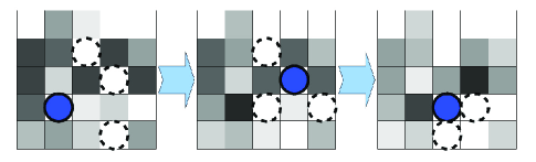
Figure 1: (Color online) Illustration of the movement of a walker in three successive time steps, where the blue fulled circle denotes the current position of the walker, and white dashed circles denote all the possible positions in the next time step. The values of $V$ in lattices are denoted by different gray scales, with pure-white for $V=V_{m}$ and dark black for $V=0$.

Because the resource in each lattice regenerates with a fixed speed, and each walker consumes at most $V_{m}$ resource at each time step, we define $r=MV_{m}/S$ to express the ratio between the total consumption of walkers and the total regeneration speed of prey resource in the landscape, where $S=N\times N$ is the area of the landscape. When $r=1$, the consumption of prey resource is equal to the regeneration speed, and the resource is in a critical status. While if $r<1$, the system has redundant resources. In our simulations, $M$ and $r$ are tunable parameters, and the value of $V_{m}$ is determined by $V_{m}=rS/M$.

Noticed that the movements in our model are not purely “deterministic” when $r<1$ or $M>1$. This probabilistic property comes from two sources: One is the random order in the updating of walkers’ positions when $M>1$, another is that a walker may have more than one choices for the next position. Purely deterministic case appears only when $r=1$ and $M=1$, in which the landscape has only one lattice with $V_{m}$ resource and the walker has to periodically repeat its early trajectories. In the cases that $r=1$ and $M>1$, although it is possible that walkers exchange their trajectories under the treating with random order, the visited time on each lattice is still strict periodic if $V_{m}$ is an integer.

III Move length Distribution

Figure 2: The trajectories of a walker in 5000 consecutive steps for different $r$. Other parameters are $M=100$ and $N=500$.

In our simulations, the size of landscape is fixed as $N=500$. We assume the prey resource is full before a group of animals come into their habitat, thus we set the initial prey resource of each lattice to be $V_{m}$, and the initial positions of walkers are randomly distributed in the landscape. Except for the case of $r=1$, our simulations show that the move length distribution gets stable after the evolution of $\frac{S}{(1.0-r)M}$ time steps, so our statistics take into account the walkers’ movement after $\frac{S}{(1.0-r)M}$ time steps. When $r=1$, the number of lattices having maximum resource is equal to the number of walkers $M$ in the steady state. In this case, each walker has to repeat its early trajectory or other walkers’ after the first $S/M$ time steps (after that time, the consumption equals regeneration), so our statistics take into account the walkers’ movement after $S/M$ time steps.

Figure 2 shows the trajectories of a walker for different $r$, where abundant long-range movements can be observed when $r$ approaches to $1$. The move length distributions $P(l)$ for different $r$ and $M$ are respectively shown in Fig. 3(a) and 3(b). When $r$ approaches 1, a scaling property of the move length distribution, say $P(l)\sim l^{-\alpha}$, can be observed. The analytical result for the move length distribution is given in the Appendix, which agrees with the simulations. As mentioned above, when $r=1$, the trajectory is periodic and thus at the last time step of a period, the walker returns to its origin, corresponding to a generally long displacement with the same order of the system size. Therefore, as shown in Fig. 3(a), when $r=1$, a peak appears at $l\approx N=500$. The dependence between the power-law exponent $\alpha$ and the parameters $r$ and $M$ are shown respectively in the two inserts of Fig. 3(a) and 3(b). Except $r=1$, $\alpha$ decreases monotonously with the increasing of $r$. For example, when $M=100$, $\alpha$ decreases from $3.3$ to $2.2$ when $r$ changes from $0.80$ to $0.99$. This range of $\alpha$ covers almost all the known real-world observations of move length distributions of animals. This result indicates that the walker is more likely to take long-range movement when the prey resource is not rich enough, which is in accordance with the experiment on the prey behavior of bumble-bees visw2 and also is supported by the resent observation on the movements patterns of marine predators Hum . Our result suggests that the animals living in a habitat with abundant prey resource will not display scaling property in their mobility.

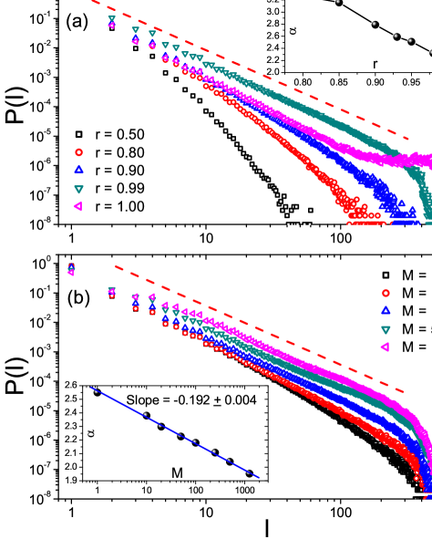
Figure 3: (Color online) (a) Move length distribution $P(l)$ for different $r$, where the inset shows the dependence between the power-law exponent $\alpha$ and $r$. Other parameters are $M=100$ and $N=500$. (b) $P(l)$ for different $M$, where the inset shows the dependence between $\alpha$ and $M$, and the blue line denotes the fitting line with slope $-0.192\pm 0.004$. Other parameters are $r=0.99$, and $N=500$. The red dashed lines in the two plots represent a power law with exponent $-2$. All the data points are averaged by 100 independent runs, each of which includes $10^{6}$ movements. The size of error bars in the two insets are smaller than the data points.

As shown in the inset of Fig. 3(b), the relation between $\alpha$ and $M$ can be well captured by logarithmic form $\alpha\sim-\ln M$. The case of $M=1$ corresponds to a solitary animal living in a fixed territory, while $M>1$ represents the case where several animals share prey resource in the same field. This result indicates that the individuals in large group are more likely to take long-range movements when the resource is not sufficiently rich.

IV Collective Movements

Figure 4: (Color online) A typical ordered marching band of walkers generated by our model when $t=50425$ ($\psi=0.57$). The red circles and black arrows denote the current positions and directions of each walkers respectively. The parameters are $r=0.99$, $M=500$ and $N=500$.

Figure 5: The periodic varying of order parameter $\psi(t)$ in three time periods with parameters $r=0.99$, $M=500$, and $N=500$.

To our surprise, collective movements are observed when $M$ is large and $r$ is close to 1, where walkers may line up one or several marching bands, and the walkers in the same marching band have similar moving directions (approximately perpendicular to the band). A typical example is shown in Fig. 4. Sometimes over half walkers are in these marching bands. Marching bands are not stable. They may suddenly emerge or disappear, may grow larger or fall into pieces.

We define an order parameter $\psi(t)$ to measure the degree of synchronization of walkers’ directions at time step $t$ as the following form Vics :

$$\psi(t)=\frac{|\sum{\vec{v}_{i}(t)}|}{\sum{|\vec{v}_{i}(t)|}},$$ (1)

where the velocity vector $\vec{v}_{i}(t)=(x_{t+1}-x_{t})\hat{x}+(y_{t+1}-y_{t})\hat{y}$, and coordinate $(x,y)$ denotes the position of the $i$-th walker, $\hat{x}$ and $\hat{y}$ respectively denote the unit of velocity on the direction $x$-axis and $y$-axis. Obviously, $\psi=1$ if all walkers have the same direction.

Figure 5 reports three typical examples of the $\psi(t)$ curves, respectively for early, middle and relatively later stages, where the quasi-periodic behavior with period length about $S/M$ can be observed. As shown in Fig. 6, when $r=0.99$, the order parameter will exceed $0.6$, indicating a strong synchronization of individual’s directions. Collective movements can be only observed when $r$ is close to $1$, which is also the condition for the emergence of scaling mobility patterns as mentioned in Section III. This property is demonstrated by the simulations shown in Fig. 6, where one can see that the steady value of order parameter is very sensitive to the parameter $r$, and when $r$ goes down from $1$, the collective movements sharply disappear.

Notice that our model does not imply any direct interaction between walkers. They are driven by the co-evolution of resource landscape and the least-action movements. This feature is far different from most known interpretations on the dynamical mechanisms of animal collective movements Vics ; Couz1 ; Couz2 ; Nagy ; Ball , yet similar to the so-called active walk process Lam1 ; Lam2 , where the macroscopic-level structure emerges from the interplay between walkers and landscape. The existence of synchronized motions is very sensitive to the value of $r$, suggesting that the food shortage may be responsible to the emergence of animal collective behaviors, which has also been observed for locusts Buhl . The existence of the scaling law in displacement distribution and the collective movements are, to our surprise, under the same condition $r\rightarrow 1$. However, these two phenomena are not the two sides of a coin, actually, they do not straightforwardly depend on each other. Whether there exists a certain mechanism underlying the co-existence is still an open question to us.

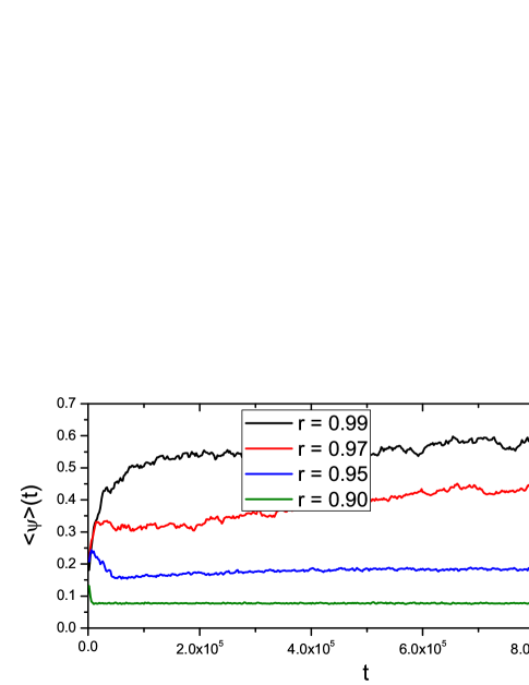
Figure 6: (Color online) The average value in each period of order parameter $\left\langle\psi\right\rangle(t)$ for different $r$, namely $\left\langle\psi\right\rangle(t)$ is the average value of $\psi$ in the range $[t-\frac{S}{2M},t+\frac{S}{2M}]$. Simulations run with parameter setting $M=500$ and $N=500$. All the data points are averaged by 10 independent runs.

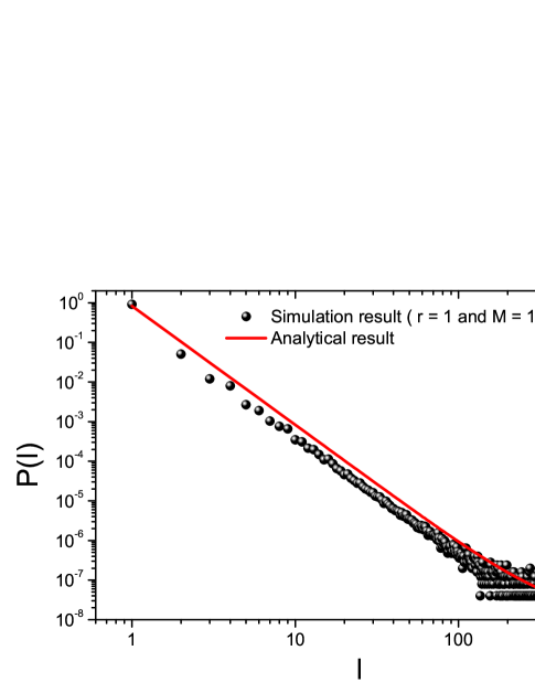
Figure 7: (Color online) Comparison of the analytical result (Eq. (A5), red line) and the simulation result (black circles) when $r=1$, $M=1$, and $N=500$. The term $l^{-1}$ plays a role only for large $l$.

V conclusions and discussions

Our model mimics the mobility patterns of many least-action walkers which prey in an landscape with regenerating ability. Scaling laws of move length distribution emerges when the regeneration speed of prey resource approaches to the critical point that the amount of resource is just enough. This result indicates that the mobility patterns of animals are sensitive to the environmental context (e.g. food resource), which is qualitatively supported by real observations visw2 ; Hum . Our model indicates that population also highly affects on the mobility patterns (see the inset of Fig. 3(b)), which is rarely discussed in early DW models. In addition, our model generates quasi-periodic collective movements with marching bands when $r\rightarrow 1$ indicating that the aggregations of animals are more likely to appear with food shortage Buhl ; Hend , which is far different from many known dynamical interpretations based on the interaction between individuals Vics ; Couz1 ; Couz2 ; Nagy ; Ball . One of the noticeable features in our results is the coexistence of both scaling mobility patterns in individual level and collective movement in population level. Both phenomena are under almost the same condition: the amount of prey resource approaches to the critical point, implying that the environment-driven mechanism may bridge the scaling individual activity patterns and global ordered behaviors.

Under different parameter settings, our results exhibit a wide and gradual spectrum of different mobility features: from the scaling movements to the random-walk-like mobility pattern, from ordered collective movements to the uncorrelated motions. These results are respectively well in agreement with different types of real-world mobility patterns of animals. However, not all the results in our model are fully addressed. Some phenomena, such as the logarithmic relation between $\alpha$ and $M$, and the microscopic mechanism in the emergence of such collective movements, are still open questions to us.

In a word, although our model is a minimum model that many real factors such as the diversity of velocity rates and the heterogeneity of environment are not considered, the results of our model are generally in agreement with many wild observations. Our model could be helpful in the understanding of the origin of both scaling mobility patterns and the ordered collective movements of animals.

Appendix A Mean-field Analysis

When $r\rightarrow 1$, the analysis can be simplified by the periodic movements. At the critical point, the period length is equal to $S/M$ and during a period, each lattice will be visited exactly once. We introduce a mean-field approximation that at any time, the unvisited lattices are evenly distributed in the space. After $\tau$ time steps, the number of unvisited lattices is $m(\tau)=S-M\tau$. Defining the normalized move length $l_{*}=l/N=lS^{-1/2}$ where $l$ is the real geometric length, the normalized probability density of the distance (move length) from an unvisited lattice to its nearest unvisited lattice after $\tau$ steps is:

$$p(l_{*},\tau)\approx[m(\tau)-1]\times 2\pi l_{*}(1-\pi l_{*}^{2})^{m(\tau)-2}.$$ (2)

The move length distribution $P(l_{*})$ during a period is the cumulation of these $p(d,\tau)$:

$$P(l_{*})\approx\frac{M}{S}\int_{0}^{S/M}p(l_{*},\tau)d\tau.$$ (3)

Substitute $m(\tau)=S-M\tau$ into Eq. (A1) and Eq. (A2), $P(l_{*})$ can be obtained as:

$$P(l_{*})\approx\frac{2\pi l_{*}}{S}[{(\ln a)}^{-2}+{(\ln a)}^{-1}]a^{-2},$$ (4)

where $a=1-\pi l_{*}^{2}$. Mostly $l_{*}\ll 1$ and thus $\ln(1-\pi l_{*}^{2})\approx\pi l_{*}^{2}$ and $a^{-2}\approx 1$. Therefore $P(l_{*})$ can be written as

$$P(l_{*})\approx\frac{2}{S}(\frac{1}{\pi}l_{*}^{-3}+l_{*}^{-1}),$$ (5)

corresponding to the distribution

$$P(l)\sim(\frac{S}{\pi}l^{-3}+l^{-1}).$$ (6)

The range of $l$ is limited from $1$ to $\sqrt{2S}$, therefore if $S$ is very large, the distribution $P(l)$ is mainly determined by the first term $\frac{S}{\pi}l^{-3}$. Figure 7 reports the analytical result Eq. (A5), which agrees with the simulation well. Notice that, the term $l^{-1}$ only show its effect for very large $l$.

References

- (1) G. M. Viswanathan, E. P. Raposo, and M. G. E. da Luz, Phys. Life Rev. 5, 133 (2008).
- (2) G. M. Viswanathan, V. Afanasyev, S. V. Buldyrev, E. J. Murphy, P. A. Prince, and H. E. Stanley, Nature 381, 413 (1996).
- (3) A.M. Reynolds, Phys. Lett. A 354, 384 (2006).
- (4) A. M. Reynolds, A. D. Smith, R. Menzel, U. Greggers, D. R. Reynolds, and D. R. Riley, Ecology 88, 1955 (2007).
- (5) G. Ramos-Fernández, J. L. Mateos, O. Miramontes, G. Cocho, H. Larralde, and B. Ayala-Orozco, Behav. Ecol. Sociobiol. 55, 223 (2004).
- (6) F. Bartumeus, F. Peters, S. Pueyo, C. Marrasé, and J. Catalan, Proc. Natl. Acad. Sci. U.S.A. 100, 12771 (2003).
- (7) D. W. Sims, E. J. Southall, N. E. Humphries, G. C. Hays, C. J. A. Bradshaw, J. W. Pitchford, A. James, M. Z. Ahmed, A. S. Brierley, M. A. Hindell, D. Morritt., M. K. Musyl, D. Righton, E. L. C. Shepard, V. J. Wearmouth, R. P. Wilson, M. J. Witt, and J. D. Metcalfe, Nature 451, 1098 (2008).
- (8) G. M. Viswanathan, S. V. Buldyrev, S. Havlin, M. G. E. da Luzk, E. P. Raposok, and H. E. Stanley, Nature 401, 911 (1999).
- (9) F. Bartumeus, J. Catalan, U. L. Fulco, M. L. Lyra, and G. M. Viswanathan, Phys. Rev. Lett. 88, 097901 (2002).
- (10) A. M. Reynolds, Phys. Lett. A 360, 224 (2006).
- (11) M. A. Lomholt, T. Koren, R. Metzler, and J. Klafter, Proc. Natl. Acad. Sci. U.S.A. 105, 11055 (2008).
- (12) D. Boyer, O. Miramontes, G. Ramos-Fernández, J. L. Mateos, and G. Cocho, Physica A 342, 329 (2004).
- (13) M. C. Santos, D. Boyer, O. Miramontes, G. M. Viswanathan, E. P. Raposo, J. L. Mateos, and M. G. E. da Luz, Phys. Rev. E 75, 061114 (2007).
- (14) A. M. Reynolds, Phys. Rev. E 78, 011906 (2008).
- (15) D. Boyer, O. Miramontes, and H. Larralde, J. Phys. A 42, 434015 (2009).
- (16) A. M. Reynolds, Phys. Rev. E 72, 041928 (2005).
- (17) D. Boyer, G. Ramos-Fernández, O. Miramontes, J. L. Mateos, G. Cocho, H. Larralde, H. Ramos, and F. Rojas, Proc. R. Soc. B 273, 1743 (2006).
- (18) N. E. Humphries, N. Queiroz, J. R. M. Dyer, N. G. Pade, M. K. Musyl, K. M. Schaefer, D. W. Fuller, J. M. Brunnschweiler, T. K. Doyle, J. D. R. Houghton, G. C. Hays, C. S. Jones, L. R. Noble, V. J. Wearmouth, E. J. Southall, and D. W. Sims, Nature 465, 1066 (2010).
- (19) T. Vicsek, A. Czirók, E. Ben-Jacob, I. Cohen, and O. Shochet, Phys. Rev. Lett. 75, 1226 (1995).
- (20) Iain D. Couzin, J. Krause, R. James, G. D. Ruxton, and N. R. Franks, J. theor. Biol. 218, 1 (2002).
- (21) Iain D. Couzin, J. Krause, N. R. Franks, and S. A. Levin, Nature 433, 513 (2005).
- (22) M. Ballerini, N. Cabibbo, R. Candelier, A. Cavagna, E. Cisbani, I. Giardina, V. Lecomte, A. Orlandi, G. Parisi, A. Procaccini, M. Viale, and V. Zdravkovic, Proc. Natl. Acad. Sci. U.S.A. 105, 1232 (2008).
- (23) M. Nagy, Z. Ákos, D. Biro, and T. Vicsek, Nature 464, 890 (2010).
- (24) L. Lam, Int. J. Bifurcat. Chaos 15, 2317 (2005) .
- (25) L. Lam, Int. J. Bifurcat. Chaos 16, 239 (2006) .
- (26) J. Buhl, D. J. T. Sumpter, I. D. Couzin, J. J. Hale, E. Despland, E. R. Miller, and S. J. Simpson, Science 312, 1402 (2006).
- (27) M. Hendrata and B. Birnir, Phys. Rev. E 81, 061902 (2010).