Chaos and universality in two-dimensional Ising spin glasses

Abstract

Recently extended precise numerical methods and droplet scaling arguments allow for a coherent picture of the glassy states of two-dimensional Ising spin glasses to be assembled. The length scale at which entropy becomes important and produces “chaos”, the extreme sensitivity of the state to temperature, is found to depend on the type of randomness. For the $\pm J$ model this length scale dominates the low-temperature specific heat. Although there is a type of universality, some critical exponents do depend on the distribution of disorder.

Glassy systems, characterized by extremely slow relaxation and resultant complex hysteresis and memory effects, are difficult to study because their dynamics encompass a great range of time scales REVIEW . Glassy materials include those without intrinsic disorder, such as silica glass, and those where quenched disorder influences the active degrees of freedom. An example of a model of the latter is the Edwards-Anderson spin glass model EA , which includes the disorder and frustration necessary to capture many of the complex behaviors seen in disordered magnetic materials. Though this prototypical model of glassy behavior was originally proposed well over 30 years ago, many aspects of it remain poorly understood. The droplet and replica-symmetry-breaking pictures of spin glasses provide distinct views of spin glass behavior YoungBook . Analytical results are rare, so numerical approaches are invaluable for both testing and motivating new ideas. But the numerics are also exceedingly difficult: computing spin glass ground states is in general a NP-hard problem Barahona . It is believed that these classes of problems require exponential computational time to solve exactly computerScience .

A fortunate special case which is not prone to this computational intractability is the two-dimensional Ising spin glass (2DISG). The Hamiltonian is $\mathcal{H}=\sum_{\langle ij\rangle}J_{ij}s_{i}s_{j}$, where the couplings ${\mathcal{J}}=\{J_{ij}\}$ are independent random variables coupling classical spins $s=\pm 1$ at sites $i$,$j$ on a square toroidal grid with $L^{2}$ sites. The randomness of the sign of $J_{ij}$ leads to competing interactions, not all of which can be satisfied. In general, such models have complex (free) energy landscapes and very slow dynamics. The most commonly-used distributions for the $J_{ij}$ are the $\pm J$ distribution where each bond value is $\pm 1$ with equal probability, or the Gaussian distribution where the $J_{ij}$ are chosen from a univariate Gaussian distribution with zero mean. One apparent difficulty in using the 2DISG as a model system is that truly long-range spin-glass order only occurs at zero temperature. However, at low enough temperature such that the correlation length $\xi$ exceeds $L$ one can study a regime of glassy behavior. In this glassy regime, the dominant spin configurations are very sensitive at large length scales to small changes in temperature or other global perturbations: this sensitivity is referred to as “chaos”.

Highly developed numerical algorithms Barahona ; GSKastCities ; SaulKardar ; GLV ; ThomasMiddletonSampling can efficiently circumvent the complexity due to disorder and frustration: ground states and finite-temperature partition functions of the 2DISG may be computed in time polynomial in $L$. Still, this model is difficult to study numerically due to strong finite-size effects. Prior to the present work, the combination of scaling ideas and exact and Monte Carlo numerical evidence had been unable to develop a full understanding of the low-temperature glassy regimes KatzgraberLeeCampbell .

In this Letter, we deduce results for the thermodynamics and droplet scaling in the glassy regime and the accompanying chaos by carrying out precise calculations at low temperatures and analyzing a variety of quantities, including the sensitivity of the entropy and energy to boundary conditions. These results give a much more consistent and detailed picture of this important model system and also have applications to other models for disorder in all dimensions. We extend fast algorithms SaulKardar ; GLV to study general disorder distributions. By employing arbitrary precision arithmetic, we have derived reliable numerical results to very low temperatures and large $L$ (beyond those attained with Monte Carlo simulations). The ground states for $\pm J$ vs. Gaussian couplings are known to have very different properties AMMP ; CHK , but it has been shown Jorg-etal that there is in a certain sense universal behavior, independent of disorder distribution, at finite temperatures. The critical behavior is universal at large length scales where the effective couplings are continuously distributed Jorg-etal , but we argue that this scaling and universal chaos applies only above a temperature-dependent crossover length scale $\ell_{x}(T)$ that itself scales differently for $\pm J$ vs. continuously-distributed bare couplings. We thereby deduce related but different critical exponents for Gaussian and $\pm J$ disorder; Ref. Jorg-etal, had instead suggested the exponents are the same. We use numerical results to support these conclusions for the 2DISG. These insights into chaos and thermodynamics will help the exploration of glassy dynamics Patch and extend the utility of this model as a standard for studying spin glasses in general.

Ordering in the glassy regime is subtle, as spin correlations have sample- and location-dependent signs. However, the magnitude of $\langle s_{i}s_{j}\rangle^{2}$ decays slowly for $|i-j|<\xi$. This ordering is evident in the effect of boundary conditions on thermodynamic quantities. We start by computing the partition function $Z_{\mathrm{P}}({\mathcal{J}})$ in a sample with periodic boundary conditions. Without additional computational effort, we then also have $Z_{\mathrm{AP}}$ for antiperiodic boundary conditions, where the horizontal bonds along a vertical column have $J_{ij}$ negated, as both are signed sums of four Pfaffians ThomasMiddletonSampling . The sample-dependent difference in free energy $F$ is $\delta F({\mathcal{J}})=-kT\ln[Z_{\mathrm{P}}({\mathcal{J}})/Z_{\mathrm{A}P}({\mathcal{J}})]$. We use finite differences over $T$ to compute the heat capacity $C$, the average energy $E$, and the entropy $S$. The sample variances $\mathrm{Var}(\delta X)$ of $\delta X\equiv X_{\mathrm{P}}-X_{\mathrm{AP}}$ for $X=F$, $E$, $S$, or $C$ help characterize the $\delta X$ distributions. In the glassy regime $L<\xi$, these differences arise from scale-$L$ relative domain walls that cross the sample: the magnitudes of $\delta X$ for these walls are taken to scale as would general droplet excitations at scale $L$ in an infinite-size system FisherHuse . We study from about $500$ to $10^{4}$ samples at each temperature. The computation of $Z$ for a $512^{2}$ sample at $T=0.1$ requires $1.6$ GB of memory and $4.4\,\mathrm{h}$ on a 2.6 GHz Opteron core. Error bars in all plots in this paper represent $\pm 1\sigma$ statistical errors.

Temperature chaos One of the most notable features of such a disordered magnet is “chaos”: a great sensitivity of the dominant spin configurations to small perturbations of the temperature BrayMoore ; FisherHuse . This sensitivity results from the delicate balance between entropy and energy in the glassy state: small temperature shifts can flip the sign of the free energy of large-scale droplets. We define a crossover length $\ell_{x}(T)$ to be the scale where the entropy of a droplet or domain wall becomes important: For scales $\ell$ with $\xi(T)>\ell>\ell_{x}(T)$, the entropy change $|\delta S|$ is typically larger than $|\delta F|/T$. A temperature change of size $\delta T<T$ can then reverse the sign of the free energy $\delta F=\delta E-T\delta S$ of the droplet or domain wall, so this is the chaotic glassy regime. Here $\delta S$ is continuously distributed, so even if the distribution of $\delta E$ is discrete, as in the $\pm J$ model, the effective couplings $\delta F(\ell)$ are continuously distributed for scales $\ell>\ell_{x}$. The natural assumption we make and verify is that when $\ell>\ell_{x}$ the exponents for the scaling with $\ell$ are independent of the bare disorder distribution. In a region of size $\ell$, for $\xi(T)>\ell>\ell_{x}(T)$ the lowest free energy droplet of size of order $\ell$ has a typical free energy $\delta F(\ell)\sim(\ell/\ell_{x})^{\theta}\delta F(\ell_{x})$, where $\theta<0$ is the usual stiffness exponent. The boundary of this droplet is a fractal domain wall with dimension $d_{f}$, and the typical $\delta S$ scales as $\delta S(\ell)\sim(\ell/\ell_{x})^{d_{f}/2}\delta S(\ell_{x})$. In verifying this picture, we will use accepted values $\theta\cong-0.28$ and $d_{f}\cong 1.274$ AMMP ; CHK ; MelchertHartmann computed in ground state simulations with Gaussian couplings, rather than fitting our data to redetermine these values.

Chaos can be seen in zero crossings of $\delta F(T)$, which imply a reordering of the values of $F$ for P and AP boundaries at scale $L$. A subset of the data for $\delta F(T)$ is displayed in Fig. 1: each curve indicates $\delta F(T)$ for a single sample (also see Sasaki-etal ). Note that in the region of appreciable $\delta F$, the number of crossings increases as $L$ increases. This helps justify the study of the 2DISG as a chaotic glassy model since a large sample will go through a large number of very different states as the temperature is lowered.

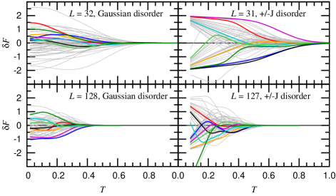
Figure 1: [color online] Chaos is evident in plots of $\delta F\equiv F_{\mathrm{P}}-F_{\mathrm{AP}}$, the change in free energy with boundary conditions, vs. temperature $T$ for both Gaussian and $\pm J$ disorder. Each panel shows curves for 50 samples of size $L^{2}$. Randomly chosen curves are highlighted to improve visibility. The number of zero crossings of $\delta F$ increases with $L$, even over the diminishing temperature range where $\delta F$ is appreciable.

Non-universal scaling and the crossover length We argue that the dependence of the crossover length $\ell_{x}$ on temperature $T$ is non-universal, so that some of the critical exponents for different disorders are distinct, though related. At short length scales, $\ell<\ell_{x}(T)$, $T\delta S<\delta F$, so that the thermodynamics at these scales is determined primarily by energetics and the $T=0$ fixed point sets the scaling behavior. In a system of size $L$ where $\ell_{x}(T)>L$, chaos is frozen out (there are typically no zero crossings in $\delta F$). This small-$\ell$ or low-$T$ nonchaotic regime is what is seen in $T=0$ simulations. It is characterized by marked differences in behavior between the $\pm J$ and Gaussian disorder distributions AMMP ; CHK .

For Gaussian disorder, the entropy of a droplet at scale $\ell<\xi$ is concentrated on the fractal domain wall with a typical total length $\ell^{d_{f}}$. The entropy difference is due to the difference in the local excitations that are affected by the introduction of this domain wall. Presuming that the local excitations at length scale $\sim 1$ have a gapless spectrum with a constant width, the fraction of the domain wall that is thermally active and contributes to the entropy difference is proportional to $T$. The entropy of the droplet, $\delta S$ is then a sum of $\sim T\ell^{d_{f}}$ terms of random sign so that $\mathrm{Var}(\delta S)\approx T\ell^{d_{f}}\sigma(T\ell^{-\theta})$ with the scaling function $\sigma(x)\rightarrow\mathrm{const.}$ as $x\rightarrow 0$. The non-chaotic regime breaks down when $T\delta S\sim T^{3/2}\ell_{x}^{d_{f}/2}\sim\ell_{x}^{\theta}\sim\delta F$, giving $\ell_{x}\sim T^{-3/(d_{f}-2\theta)}$ for Gaussian disorder.

For $\pm J$ disorder and low $T$, the entropy of a scale-$\ell$ droplet with $\ell<\ell_{x}(T)$ is found to scale as $\delta S\sim\ell^{\theta_{S}}$. The value of $\theta_{S}$ is fixed by the $T=0$ domain wall entropy due to zero-energy spin rearrangements, and estimated numerically to be $\theta_{S}\cong 0.5$ LukicEtAlJStat . Additionally, the typical (free) energy of excitations at zero temperature has been found to be $\mathcal{O}(1)$, independent of $L$ AMMP ; CHK , which we have verified: fitting $\delta F(T=0)$ to a simple power law over $L=32\rightarrow 256$ gives an exponent with magnitude less than $0.015$. The crossover scale $\ell_{x}$ therefore occurs when $\delta E\sim\delta F\sim T\delta S\sim\mathcal{O}(1)$, giving $\ell_{x}\sim T^{-1/\theta_{S}}$, so that Gaussian and $\pm J$ distributions have distinct scaling. Crucially, this also means $\delta F(\ell_{x})\sim\mathcal{O}(1)$, in contrast with $\delta F(\ell_{x})\sim\ell_{x}^{\theta}$ for the Gaussian case; this introduces an additional source of nonuniversality.

For Gaussian disorder, the free energy magnitude scales as $\mathrm{Var}(\delta F)\approx\ell^{2\theta}\phi(T\ell^{-\theta})$ with scaling function $\phi(x)\rightarrow\mathrm{const.}$ as $x\rightarrow 0$ BrayMoore ; FisherHuse . The correlation length $\xi(T)$ is set by the scaling argument $x=\mathcal{O}(1)$, which gives $\xi\sim T^{-\nu_{G}}$ with $\nu_{G}=-1/\theta\cong 3.5$. For $\pm J$ disorder, low $T$ and $\ell>\ell_{x}(T)$ in the universal, chaotic regime, $\mathrm{Var}(\delta F)\approx(\ell/\ell_{x})^{2\theta}\phi[T(\ell/\ell_{x})^{-\theta}]$ with the same universal scaling function $\phi(x)$. But here the argument of the scaling function has different $T$-dependence from what it has with continuously-distributed disorder. As a result the correlation length scales with a different exponent, $\xi\sim T^{-\nu_{\pm}}$, with $\nu_{\pm}=1/\theta_{S}-1/\theta\cong 5.5$.

We computed $\mathrm{Var}(\delta F)$ for samples chosen independently at each temperature. We directly test the scaling forms expected for $\delta F$ by a finite-size scaling collapse of this data with no free parameters. For the Gaussian data, shown in Fig. 2(a), we find agreement with the expected exponents and thus a good estimate of the scaling function $\phi(x)$. We plot the data for the $\pm J$ model using its expected scaling in Fig. 2(b), where the same scaling function $\phi(x)$ with only constant rescaling should appear. Although the expected deviations are apparent at low temperature and small $L$ where $L<\ell_{x}(T)$ and at $T=\mathcal{O}(1)$, we see a trend towards good collapse of the data for larger $L$, consistent with the proposed new scaling, and similar curves for the $\phi(x)$. It appears that for $\pm J$ disorder the universal regime of $L>\ell_{x}(T)$ and $T<\mathcal{O}(1)$ does not emerge until $L\apprge 100$.

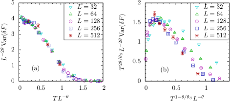
Figure 2: [color online] (a) Scaling collapse for the variance of the twist free energy, $\mathrm{Var}(\delta F)$, for Gaussian disorder, with $\mathrm{Var}(\delta F)L^{-2\theta}$ plotted vs. $TL^{-\theta}$. (b) Scaling collapse for $\pm J$ disorder that accounts for the crossover-length $\ell_{x}(T)$ so that convergence to the same universal scaling function is expected (up to overall scales for $T$ and $L$). There are no fitted exponents in these plots: accepted values $\theta=-0.28$ and $\theta_{S}=0.50$ are used.

The chaos exponent The rate of change of $\delta F$ with $T$ in an individual sample is given by the entropy difference, $\delta S=-\frac{\partial\,\delta F}{\partial T}$. Thus, in the chaotic regime, the temperature change needed to change the sign of $\delta F$ is typically $\Delta T\sim\delta F/\delta S$. Using the above expressions for $\delta F$ and $\delta S$, the rate of sign changes in $\delta F$ as $T$ is varied for Gaussian disorder is given by $|\delta S|/|\delta F|\sim L^{\zeta^{\prime}_{G}}\kappa_{G}(TL^{1/\nu_{G}})$ with chaos exponent $\zeta^{\prime}_{G}=(d_{f}+1/\nu_{G})/2$ and scaling function $\kappa(x)\propto x^{1/2}$ at small argument. For $\pm J$ disorder, $T\delta S(\ell_{x})\sim\mathcal{O}(1)$, so that in the chaotic regime $\delta S\sim(\ell/\ell_{x})^{d_{f}/2}/T$ and the rate of sign changes is $|\delta S|/|\delta F|\sim(L/\ell_{x})^{d_{f}/2-\theta}T^{-1}\kappa_{\pm}(TL^{1/\nu_{\pm}})$, with $\kappa_{\pm}$ constant for small arguments. This gives $\zeta^{\prime}_{\pm}=(d_{f}/2-2\theta)[\theta_{S}/(\theta_{S}-\theta)]$. Though these two expressions for $\zeta^{\prime}$ are quite different, they are predicted to have similar values: $\zeta^{\prime}_{G}=0.78(1)$ and $\zeta^{\prime}_{\pm}=0.77(2)$ (Fig. 3).

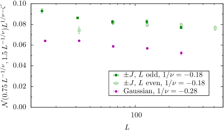
Figure 3: [color online] A plot of the scaled crossing rate $L^{-\zeta^{\prime}}\mathcal{N}(T_{1},T_{2})/(T_{2}-T_{1})$, where the average number of zero crossings for $\delta F$ in the interval $T_{1}<T<T_{2}$ is $\mathcal{N}(T_{1},T_{2})$ HuseKo , using $(T_{1},T_{2})=(0.75\,L^{-1/\nu},1.5\,L^{-1/\nu})$. The rate is expected to scale with $L$ as $\propto L^{\zeta^{\prime}}$, with $\zeta^{\prime}_{G}=0.78(1)$ and $\zeta^{\prime}_{\pm}=0.77(2)$. The expected nearly constant scaled rate is seen for both Gaussian and bimodal disorder.

Specific heat The behavior of the specific heat $C$ for $T\rightarrow 0$ in a 2DISG is dominated by the smallest thermally active droplets that have nonzero energy FisherHuse . If the disorder distribution is continuous, these are the smallest droplets of size $\mathcal{O}(1)$ and energy of order $T$. They have a density proportional to $T$ and contribute a linear term in the low $T$ specific heat: $C\sim T$.

For $\pm J$ disorder, on the other hand, the droplets with the lowest nonzero energy have $\delta E=\mathcal{O}(1)$. Such droplets with size $\ell<\ell_{x}(T)$ have $\delta F>T$ at low $T$ and are not thermally active. Thus at low temperature $T$ the smallest active droplets with nonzero energy are of size $\ell_{x}(T)$. These active droplets each contribute $\sim 1/T^{2}$ to the specific heat and have density $T/\ell_{x}^{2}(T)$ so the specific heat scales as $C\sim T^{2/\theta_{S}-1}$. In an a average over finite-sized samples this power-law specific heat is cut off at the lowest temperatures when the size $\ell_{x}(T)$ of these active droplets exceeds $L$. This produces the low-$T$ finite-size scaling form $C\approx T^{2/\theta_{S}-1}c(TL^{\theta_{S}})$, where $c(x)$ is a scaling function that goes to a constant for large argument (for temperatures where $\ell_{x}(T)\ll L\ll\xi(T)$). Our $\pm J$ specific heat data are shown in this scaling form in Fig. 4. The intermediate temperature regime that corresponds to the power-law specific heat only appears for $L>100$. In fact, our data for intermediate temperatures, $T\approx 0.35$, are entirely consistent with previously published work KatzgraberLeeCampbell , which saw an effective exponent $\alpha\approx-4.2$, with $C\sim T^{-\alpha}$, but the effective exponent crosses over to lower values as $T$ decreases.

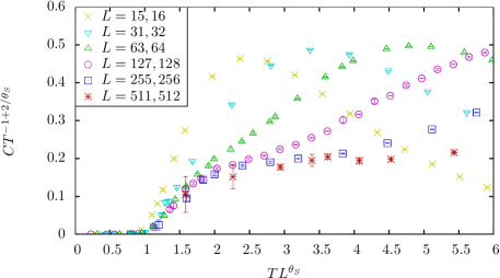
Figure 4: [color online] A scaling plot for the heat capacity $C$ for the $\pm J$ spin glass. The scaled heat capacity per spin, $CT^{1-2/\theta_{S}}$ is plotted as a function of the scaled temperature $TL^{\theta_{S}}$ for samples of size $L$ with the value of $\theta_{S}=0.50$ consistent with the zero temperature scaling of the entropy of domain walls, $\delta S\sim L^{\theta_{S}}$ LukicEtAlJStat . This collapse is consistent with the “bulk” heat capacity being due to excitations of minimal size $\ell_{x}\sim T^{-1/\theta_{S}}$.

In addition to the leading terms that we discuss above and detect in our numerical results, there are weaker singular contributions to $C$ that result from the diverging $\xi(T)$ as $T\rightarrow 0$ that are also there in principle, although they will be extremely difficult to detect. Standard hyperscaling at $T=0$ predicts a contribution that scales as $C\sim T^{-\alpha}\sim T^{2\nu}$ Jorg-etal , but the chaos changes this, making this contribution larger at low $T$. The contribution to the specific heat from droplets of scale $\ell\leq\xi(T)$ is the product of their density $\sim 1/\ell^{2}$, the fraction that are thermally active $\sim T/\delta F(\ell)$ and the average contribution of such an active droplet to the heat capacity $\sim(\delta E_{\mathrm{act}}(\ell)/T)^{2}$. For standard hyperscaling, the last two factors are of order one for $\ell=\xi(T)$, but the chaos instead makes the last term larger. The subdominant contribution to $C$ for Gaussian disorder from scale $\xi$ is $C_{\mathrm{sing}}\sim T^{2\nu_{G}(1-\zeta^{\prime}-\theta)}$, since $\delta E_{\mathrm{a}ct}/T\sim\delta S_{\mathrm{act}}\sim\ell^{\zeta^{\prime}+\theta}$. However, the first factor always wins, keeping the smallest thermally active droplets with $\delta E>0$ dominant in the specific heat.

Discussion Precise numerical calculations have allowed us to test new scaling relations for the thermodynamics of the 2DISG in detail and to clearly demonstrate non-universality and study its origin. The large values of $\nu$ (and long crossover lengths for $\pm J$ disorder) necessitate using large systems to see the scaling behavior. Even though we assumed that scaling in the chaotic regime is weakly universal with the same values of $\theta$ and $d_{f}$ at any given $T$, our results show that the critical exponents are nevertheless different for Gaussian and $\pm J$ disorder, due to temperature- and disorder- dependent crossover length scales. We predict a violation of hyperscaling due to chaos, which is a general phenomenon that is present in higher dimensions as well. These results will lead to further work on the thermodynamics and glassy dynamics of this glassy model at low temperature.

This work was supported in part by NSF grants DMR-1006731 and DMR-0819860. We are grateful for the use of otherwise idle time on the Syracuse University Gravitation and Relativity computing cluster, supported in part by NSF grant PHY-0600953, to generate almost all of the numerical results, and additional time on the Hypatia cluster (supported in part by NSF DMR-0645373) and the Brutus cluster of ETH Zurich. We thank Helmut Katzgraber for helpful comments.

References

- (1) K. Binder and A. P. Young, Rev. Mod. Phys. 38, 801 (1986).
- (2) F. Edwards and P. W. Anderson, J. Phys. F 5, 965 (1975).
- (3) “Spin Glasses and Random Fields”, A. P. Young, ed. (World Scientific, Singapore, 1998).
- (4) F. Barahona, J. Phys. A 15 3241 (1982).
- (5) C. H. Papadimitriou, Computational Complexity (Addison-Wesley, Reading, MA, 1994).
- (6) C. K. Thomas and A. A. Middleton, Phys. Rev. B 76 220406(R) (2007).
- (7) L. Saul and M. Kardar, Phys. Rev. E 48, R3221 (1993).
- (8) A. Galluccio, M. Loebl and J. Vondrak, Phys. Rev. Lett. 84, 5924 (2000).
- (9) C. K. Thomas and A. A. Middleton, Phys. Rev. E 80, 046708 (2009).
- (10) H. G. Katzgraber, L. W. Lee and I. A. Campbell, Phys. Rev. B 75, 014412 (2007).
- (11) C. Amoruso, et al., Phys. Rev. Lett. 91, 087201 (2003).
- (12) I. A. Campbell, A. K. Hartmann, and H. G. Katzgraber Phys. Rev. B 70, 054429 (2004).
- (13) T. Jörg, et al., Phys. Rev. Lett. 96, 237205 (2006).
- (14) C. K. Thomas, O. L. White and A. A. Middleton, Phys. Rev. B 77, 092415 (2008).
- (15) D. S. Fisher and D. A. Huse, Phys. Rev. B 38, 386 (1988).
- (16) A. J. Bray and M. A. Moore, Phys. Rev. Lett. 58, 57 (1987).
- (17) M. Sasaki, et al., Phys. Rev. Lett. 95, 26203 (2005).
- (18) O. Melchert and A. K. Hartmann, Phys. Rev. B 76 174411 (2007).
- (19) D. A. Huse and L.-F. Ko, Phys. Rev. B 56, 14597 (1997).
- (20) J. Lukic, et al., J. Stat. Mech. L10001 (2006).
- (21) C. K. Thomas, D. A. Huse, and A. A. Middleton (unpublished).