Aging and stationary properties of non-equilibrium symmetrical three-state models

Abstract

We consider a non-equilibrium three-state model whose dynamics is Markovian and displays the same symmetry as the three-state Potts model, i.e., the transition rates are invariant under the permutation of the states. Unlike the Potts model, detailed balance is in general not satisfied. The aging and the stationary properties of the model defined on a square lattice are obtained by means of large-scale Monte Carlo simulations. We show that the phase diagram presents a critical line, belonging to the three-state Potts universality class, that ends at a point whose universality class is that of the voter model. Aging is considered on the critical line, at the voter point and in the ferromagnetic phase.

1 Introduction

The critical behavior of equilibrium systems can be classified according to universality classes that are characterized by a small number of features such as symmetries, conservation laws and dimensionality [1]. The universality classes of non-equilibrium systems without detailed balance are also characterized by these features and possibly others [2, 3, 4, 5]. It seems that any universality class that encompasses systems in equilibrium includes also non-equilibrium systems although the reverse is not true. The universality class of directed percolation for instance does not include systems in equilibrium. In other words, some classes of universality comprehend equilibrium as well as non-equilibrium systems and in this case we may say that the lack of detailed balance is irrelevant. Other classes are constituted only by non-equilibrium systems and the lack of detailed balance is a relevant property.

Here we study a two-parameter non-equilibrium model that belongs to the universality class of the three-state Potts model. As happens to the latter, the non-equilibrium model studied here displays a continuous phase transition from an ordered to a disordered phase. As one varies the parameters along the critical line separating the ordered and disordered phases, the model leaves the Potts universality class and displays a crossover to the non-equilibrium universality class of the voter model at the terminus of the critical line. The model is studied on a regular square lattice and the transition probabilities depend only on the four neighbors of a given site. We set up the most general model obeying the same symmetry as the equilibrium Potts model. In this case the symmetry of the model is identified as the symmetry of the transition rates in contrast to equilibrium models for which the symmetry of the model is identified as the symmetry of the Hamiltonian. The most generic model has five parameters but here we focus on a certain two-dimensional section of the space of parameters.

The model is presented in section 2. The critical line and the critical exponents in the stationary state are determined by Monte Carlo simulations and the results are presented in the section 3. Finally, the aging of the model when quenched from the high-temperature phase is studied in section 4. In order to define a response function, the coupling to an external field is implemented by an appropriate modification of the transition rate as detailed in the Appendix.

2 Model

We consider a general non-equilibrium three-state model on a square lattice with full symmetry $Z_{3}$. Any permutation of the three states leaves the transition probabilities invariant. On a square lattice, in which each site has four nearest neighbor sites, the most general model has five parameters as shown in table 1. Several non-equilibrium models as well as the stochastic equilibrium Potts model [6] are particular cases of this general model.

Among them we found the non-equilibrium majority Potts model [7, 8] defined in such a way that a site takes the state of the majority of the neighboring sites with probability $p$ and any one of the other state with probability $(1-p)/2$. With our definition, it is recovered when

$$p_{1}=p_{2}=p_{3}=p_{4}=1-2p_{5}=p.$$ (1)

This model does not obey detailed balance and therefore displays irreversibility at the stationary state. It has been shown [7] that it presents a phase transition from a disordered (paramagnetic) to an ordered state (ferromagnetic), for sufficiently large values of $p$, which is similar to the phase transition in the ordinary equilibrium three-state Potts model. Both models are in the same universality class with the critical exponents $\nu=5/6$ and $\beta=2/15$.

The equilibrium Potts model [6] with a Glauber dynamics is recovered when the parameters are such that detailed balance is fulfilled. This occurs when

$$p_{1}=\frac{r^{4}}{2+r^{4}},$$ (2)

$$p_{2}=\frac{r^{3}}{1+r+r^{3}},\qquad\qquad p_{5}=\frac{r}{1+r+r^{3}},$$ (3)

$$p_{3}=\frac{2r^{2}}{1+2r^{2}},\qquad\qquad p_{4}=\frac{r}{2+r},$$ (4)

where $r=e^{\beta J}$ and $J$ is the nearest-neighbor exchange coupling of the Potts model.

Another particular case is the so called linear voter model obtained when we set

$$p_{1}=\frac{1}{3}(1+2\gamma),$$ (5)

$$p_{2}=\frac{1}{3}(1+\frac{5}{4}\gamma),\qquad\qquad p_{5}=\frac{1}{3}(1-\frac{1}{4}\gamma),$$ (6)

$$p_{3}=\frac{1}{3}(2+\gamma),\qquad\qquad p_{4}=\frac{1}{3}(1+\frac{1}{2}\gamma).$$ (7)

This model is particularly interesting because it can be solved exactly [16]. It displays a disordered phase except at $\gamma=1$ corresponding in our notations to

$$p_{1}=1,\qquad p_{2}=3/4,\qquad p_{5}=1/4,\qquad p_{3}=1,\qquad p_{4}=1/2.$$ (8)

In this particular case it is called the voter Potts model and undergoes a first-order phase transition with a magnetization jump but divergences of susceptibility and correlation length associated to critical exponents $\gamma=1$ and $\nu=1/2$.

Table 1: Transition probabilities of the general non-equilibrium three-state model on a square lattice. The first column shows the states of the four nearest neighbor sites. The first row shows the final states. The parameters $p_{1}$, $p_{2}$, $p_{3}$, $p_{4}$, and $p_{5}$ are restricted to the interval [0,1]. The other transition probabilities are obtained by permutation of the states.

	1	2	3
1 1 1 1	$p_{1}$	$(1-p_{1})/2$	$(1-p_{1})/2$
1 1 1 2	$p_{2}$	$p_{5}$	$1-p_{2}-p_{5}$
1 1 2 2	$p_{3}/2$	$p_{3}/2$	$1-p_{3}$
1 1 2 3	$p_{4}$	$(1-p_{4})/2$	$(1-p_{4})/2$

The general model includes also models with absorbing states. Due to the Potts symmetry these models display three absorbing states represented by a lattice full of each of the three states. The class of absorbing models occurs when $p_{1}=1$. A particular case of this class is the Potts voter model already mentioned and defined by Eq. (8).

Here we are interested in a subclass of models that interpolates between the majority vote model, defined by (1), and the voter model (8). This subclass of models is defined by a set of two parameters $a$ and $b$ that corresponds to a section of the full space spanned by the parameters $\{p_{i}\}$. The relation between $a$, $b$ and $\{p_{i}\}$ is given by

$$p_{1}=b,\qquad\qquad p_{3}=b,\qquad\qquad p_{4}=a,$$ (9)

$$p_{2}=b\left(1+\frac{a-b}{2}\right),\qquad\qquad p_{5}=\frac{b}{2}(1-a)+\frac{1}{2}(1-b)^{2}.$$ (10)

The phase diagram, to be presented shortly, is therefore a bidimensional section of the full five-dimensional space. The majority Potts model is recovered when $a=b$. When $b=1$, we get a model with absorbing state with the particular case of the voter Potts model occurring at $b=1$ and $a=1/2$.

The construction that is presented above is easily generalized to any number of states $q$ of the Potts model. Such a construction has already been proposed in the case $q=2$, i.e., with the symmetry of the Ising model [9, 10]. Among the models appearing as special case in the $q=2$ construction, voter and linear models were studied analytically [11] and the Glauber-Ising model was studied by Monte Carlo simulations [9, 10, 12, 13]. Aging was also considered [14].

3 Critical properties in the stationary state

In this section, we give numerical evidences that the phase diagram in the $a-b$ plane presents a critical line separating a ferromagnetic phase from a paramagnetic one and ending at the point $a=1/2$ and $b=1$. Excluding this special point, the universality class of all points along the critical line is that of the three-state Potts model. Along the line $b=1$, the system undergoes a dynamical absorbant-active phase transition. The intersection of the two lines, at $a=1/2$ and $b=1$, belongs to the voter universality class.

3.1 Numerical methodology

The phase diagram of the model was investigated by means of Monte Carlo simulations on a square lattices with $N=L^{2}$ sites and periodic boundary conditions. The system is initially prepared in the ferromagnetic state. $n_{\rm therm.}$ Monte Carlo steps (MCS) are performed to let the system reach a stationary state. Then $n_{\rm iter.}$ MCS are made to sample the stationary probability distribution. The order parameter, abusively called magnetization in the following, is measured for a given spin configuration $\sigma=\{\sigma_{i}\}$ as

$$m(\sigma)={q\rho_{\rm max}(\sigma)-1\over q-1},$$ (11)

where $q=3$ is the number of Potts states and $\rho_{\rm max}$ is the density of spin in the majority state. If we denote by $\sigma_{\rm max}$ the majority state (among the $q$ possible states) then

$$\rho_{\rm max}(\sigma)=\!{1\over N}\sum_{i}\delta_{\sigma_{i},\sigma_{\rm max}}.$$ (12)

Of particular interest for the determination of the critical line are the susceptibility

$$\chi=N(\langle m^{2}\rangle-\langle m\rangle^{2}),$$ (13)

and the Binder cumulant $U$

$$U=1-{\langle m^{4}\rangle\over 3\langle m^{2}\rangle^{2}}.$$ (14)

In addition to the susceptibility and Binder cumulant, we also evaluated the correlation length. For a finite system, the correlation length $\xi$ is finite so that the spatial correlation function decays exponentially,

$$C(\vec{r},\vec{r}^{\prime})=\langle m(\vec{r})m(\vec{r}^{\prime})\rangle\sim\langle m\rangle^{2}+Ae^{-|\vec{r}-\vec{r}^{\prime}|/\xi},$$ (15)

where $m(\vec{r}_{i})=(q\delta_{\sigma_{i},\sigma_{\rm max}}-1)/(q-1)$ is the local magnetization on site $i$. The CPU time required to compute the full spatial correlation function being prohibitive, we restricted ourselves to the first coefficient of its Fourier transform

$$C(\vec{k})={1\over\sqrt{N}}\sum_{\vec{k}}C(0,\vec{r})e^{i\vec{k}.\vec{r}}\sim{B\over 1/\xi^{2}+k^{2}+\alpha k^{4}+\ldots},$$ (16)

which is efficiently computed as

$$C(\vec{k})=\langle m(\vec{k})m(-\vec{k})\rangle=\langle|m(\vec{k})|^{2}\rangle,$$ (17)

where $m(\vec{k})$ is the Fourier transform of the magnetization

$$m(\vec{k})={1\over\sqrt{N}}\sum_{\vec{r}}m(\vec{r})e^{i\vec{k}.\vec{r}}.$$ (18)

Finally, the correlation length is estimated as

$$\xi\simeq{1\over k_{\rm min}}\sqrt{{C(0)\over C(k_{\rm min})}-1},$$ (19)

where $k_{\rm min}=(2\pi/L,0)$ is the smallest wavevector on the lattice in order to minimize the terms $\alpha k^{4}+\ldots$ and to be able to neglect them. In the paramagnetic phase, $C(0)=\langle m^{2}\rangle$ while in the ferromagnetic phase, one has to remove the unconnected term, i.e. $C(0)=\langle m^{2}\rangle-\langle m\rangle^{2}$. Practically, we will use always the second definition unless it leads to a negative value which often occurs in the paramagnetic phase because of the numerical instability of the difference $\langle m^{2}\rangle-\langle m\rangle^{2}$ between two small and noisy values.

In order to adjust the number of iterations $n_{\rm therm.}$ and $n_{\rm iter.}$ and to calculate error bars, we measured autocorrelation functions of $m^{2}$ defined as:

$$C(t,s)=m^{2}(t)m^{2}(s)-\langle m^{2}\rangle^{2}.$$ (20)

Assuming that these autocorrelation functions decay exponentially, $C(t,s)\sim e^{-|t-s|/\tau}$, the so-called integrated relaxation time is estimated as

$$\tau={1\over n_{\rm iter}}\sum_{t,s=1}^{n_{\rm iter}}C(t,s)\sim\int e^{-u/\tau}du,$$ (21)

$n_{\rm therm.}$ and $n_{\rm iter.}$ are always chosen larger than $20\tau$ and $10^{4}\tau$ respectively. Since $\tau$ gives a measure of the number of MCS required to obtain a spin configuration uncorrelated from the initial one, the number of effective uncorrelated MCS is of order $N/\tau$. As a consequence, the error bars can be computed for an observable $X$ as

$$\Delta X=\sqrt{\tau{\langle X^{2}\rangle-\langle X\rangle^{2}\over N}}.$$ (22)

The error bars only measure the statistical fluctuations of the data. To detect and potentially avoid systematic deviations due to metastable or absorbing states, the simulation is repeated $n_{\rm conf}=20$ times for all lattice sizes and the observables are averaged over these configurations. In the following, we will denote for simplicity $\langle X\rangle$ this double average.

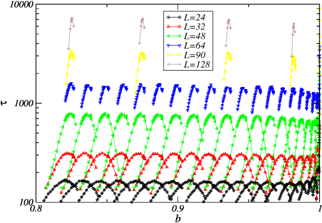
Figure 1: Auto-correlation time $\tau$ as a function of $b$. The different peaks corresponds to distinct values of $a$. The different colors correspond to lattice sizes $L=24$, 32, 48, 64 and for five values of $a$ only $L=90$ and 128.

The difficulty of these simulations is that the relaxation time $\tau$ is expected to grow very fast with the lattice size, i.e. as $\tau\sim L^{z}$ where the dynamical exponent is of order $z\simeq 2$ (the dynamical exponent will be determined by finite-size scaling at the end of the next section) since the dynamics is always local (see figure 1). At the largest lattice size $L=128$, up to $n_{\rm conf}=20$ simulations of $n_{\rm iter.}=7.3\times 10^{7}$ MCS each have been performed. Despite the computational effort devoted to these simulations, we cannot hope to reach the same accuracy as equilibrium simulations for the three-state Potts model for which a cluster algorithm is available (which is not the case for our more general model for which detailed balance does not hold). For our largest lattice size, $L=128$, the auto-correlation time reaches the maximum value of $\tau\simeq 7231$ on the critical line belonging to the $q=3$-Potts universality class while it is only $\tau\simeq 25$ for the Potts model with the Swendsen-Wang algorithm [15].

3.2 Determination of the critical line

The critical line is determined from the maximum of the susceptibility. We have considered twenty values of the parameter $a$ between $a=1/2$ and $a=1$ and lattice sizes $L=16$, 20, 24, 32, 48 and 64. For five specific values of $a$, we made additional simulations for lattice sizes $L=90$ and $128$. For each value of $a$ and $L$, we have performed Monte Carlo simulations for several values of $b$ as shown in figure 2. Additional simulations were performed around the maxima of $\chi$. In the neighborhood of these maxima, we interpolated $\chi(b)$ with a polynomial of degree two to improve the accuracy on the location of the maximum. For each lattice size $L$ and each value $a$, we thus defined a pseudo-critical parameter $b_{c}(a,L)$ as shown in figure 3. These values are finally extrapolated in the thermodynamic limit $L\rightarrow+\infty$ with a polynomial of degree two in $1/L$. The final critical line $b_{c}(a)$ is presented in figure 3.

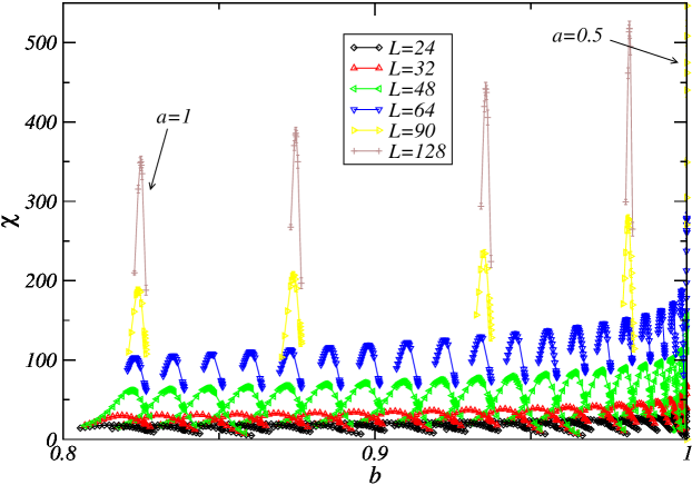
Figure 2: Susceptibility $\chi$ as a function of $b$. The different peaks corresponds to distinct values of $a$. The different colors correspond to lattice sizes $L=24$, 32, 48, 64 and for five values of $a$ only $L=90$ and 128.

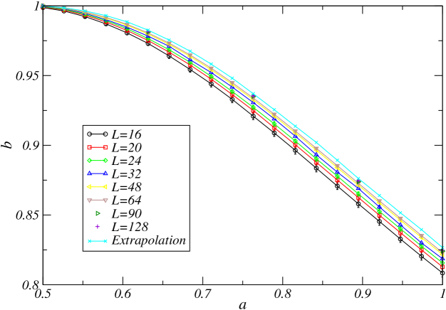
Figure 3: Critical line determined from the maximum of the susceptibility $\chi$. Different lines correspond to distinct lattice sizes and to the thermodynamic limit extrapolation.

The same analysis has been applied to the correlation length $\xi$ and to the correlation time $\tau$. However, since the analysis based on the susceptibility $\chi$ turned out to be the most precise, we did not perform further simulations to refine the location of the maxima of $\xi$ and $\tau$.

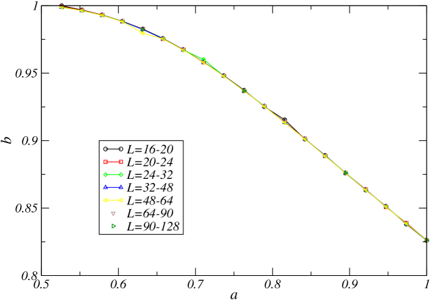
Figure 4: Critical line determined from the crossing of the Binder cumulant $U$ for distinct values of the lattice size.

We have also determine the critical line from the crossing of the Binder cumulant $U$ at two different lattice sizes (figure 4). For each value of $a$ and for each pair of successive lattice sizes, we used a linear interpolation to get a trial estimation of the crossing position. Next, we used five points around the preliminary estimation to interpolate a polynomial of degree two from which we get a more precise estimation. Note that for $a=1/2$, the curves do not cross because $b_{c}=1$. Despite the fact that the crossing point does not depend significantly on the lattice size, a more precise determination of $b_{c}$ is forbidden by statistical fluctuations, which are greater than those of the susceptibility and thus give a less accurate extrapolation. In the following, we will use the determination of the critical line given by the susceptibility.

3.3 Critical behavior along the transition line

We have used finite-size scaling analysis to determine the critical exponents. Figure 5 shows the maximum of the susceptibility $\chi$ as a function of the lattice size $L$ for several values of the parameter $a$. According to finite size scaling, the maximum of $\chi$ behaves as

$$\chi\sim L^{\gamma/\nu}.$$ (23)

We see from figure 5 that the case $a=1/2$ differs significantly from the other cases. The ratio $\gamma/\nu$ is estimated from the slope of the log-log plot of $\chi$ versus $L$. The values obtained by this procedure are plotted as a function of $a$ as shown in figure 6. For $a=1/2$ we get an exponent compatible with the value $\gamma/\nu=2$ of the voter model [16]. For $a>1/2$, the effective critical exponent displays a plateau around $1.78(3)$ along the critical line, i.e., still slightly above the value $\gamma/\nu\simeq 1.733$ expected for the three-state Potts model. The effective exponent decreases when removing the smallest lattices but with the lattice sizes that we have been able to considered, the exact value $\gamma/\nu=1.733$ is not reached yet.

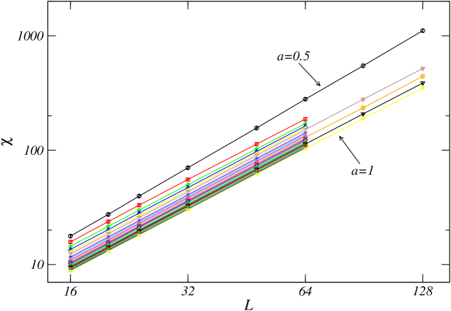
Figure 5: Maximum of the susceptibility $\chi$ as a function of the lattice size $L$. Different curves correspond to distinct values of the parameter $a$.

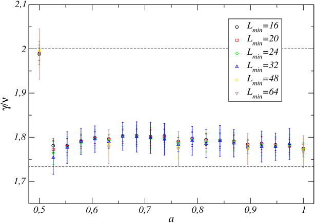
Figure 6: Effective exponent $\gamma/\nu$ obtained by interpolation of the susceptibility as a function of $a$. The dotted lines correspond to $\gamma/\nu=2$ (voter model) and to $\gamma/\nu\simeq 1.733$ (three-state Potts model). The different symbols correspond to exponents obtained by power-law interpolation when taking into account lattice sizes $L\geq L_{\rm min}$ only.

At the point $a=1/2$, corresponding to the voter model, the susceptibility presents a logarithm correction to the dominant behavior [16],

$$\chi\sim\big{[}(1-b)\ln(1-b)\big{]}^{-1}.$$ (24)

In figure 7 we have plotted $\chi$ versus $[(1-b)\ln(1-b)]^{-1}$ for several values of the lattice size $L$. The deviation from a linear behavior is due to finite size effects. Indeed, the curves become linear over a wider range of values of $[(1-b)\ln(1-b)]^{-1}$ as one increases $L$.

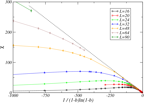
Figure 7: Susceptibility $\chi$ as a function of $[(1-b)\ln(1-b)]^{-1}$ at $a=1/2$ (voter model).

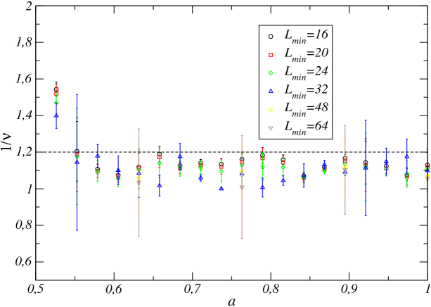
Figure 8: Exponent $\nu$ obtained by interpolation as a function of $a$. The dotted line correspond to $\nu=5/6$ (three-state Potts model). The different symbols correspond to exponents obtained by power-law interpolation when taking into account only the lattice sizes $L\geq L_{\rm min}$.

To determine the exponent $\nu$, we have used the position $b_{c}(a,L)$ of the maximum of the susceptibility and the value $b_{c}(a,\infty)$ obtained by extrapolation. The finite-size deviation is expected to behave as

$$b_{c}(a,L)-b_{c}(a,\infty)\sim L^{-1/\nu}.$$ (25)

The exponent $\nu$ can then be obtained from the log-log plot of the deviation versus $L$. Our numerical estimates are shown in figure 8. The average value $1/\nu=1.10(13)$ leads to $\nu=0.91(10)$ slightly larger, but not incompatible with the value $\nu=5/6$ of the three-state Potts model.

The scaling of the Binder cumulant is presented on figure 9. For parameters $a$ smaller than $a\sim 0.7$, a strong cross-over is observed: the data do not fall on a single curve for different values of $a$. For $a>0.7$, the cross-over effects become smaller than the error bars and all data fall on a unique curve, providing further evidence that the universality class is the same along the critical line, at least for $a>0.7$. From the curve, we can see that the universal value of the Binder cumulant is $U=0.615(5)$ in agreement with [8].

On figure 10, the scaling function ${\cal F}_{\xi}$ of the correlation length $\xi$ such that

$$\xi\sim L{\cal F}_{\xi}\big{(}(b-b_{c}(a))L^{\nu}\big{)},$$ (26)

is plotted for values of $a$ larger than $0.7$. Again a strong cross-over is observed below $a\sim 0.7$. In the finite-size regime $(b-b_{c}(a))L^{\nu}<0.1$, the scaling function displays a plateau at a value $\xi/L$ that is expected to be universal. The values of $a$ considered in the plot leads to a compatible value of $\xi/L$. Note that our value of $\xi/L$ differs from that given in ref. [15] for the 3-state Potts model because of a different correlation function used for the definition of the correlation length $\xi$.

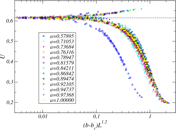
Figure 9: Scaling of the Binder cumulant $U$ in the critical line. All data points for lattices sizes $L=24,32,48,64,90$ and $128$ and for values of $a$ above $0.7$ were used. The data for $a\simeq 0.57$ is also plotted (blue triangles) to show the cross-over with the voter point. The two branches, above and below the dashed horizontal line, correspond to high and low-temperature phases.

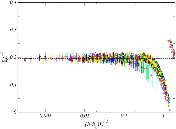
Figure 10: Scaling of the correlation length $\xi$ on the critical line. All data points for lattices sizes $L=24,32,48,64,90$ and $128$ and for twelve values of $a$ above $0.7$ were used. The points on the second branch at the right of the figure correspond to data in the paramagnetic phase for which for numerical reasons (see previous section), the definition of $\xi$ has to be chosen differently.

To determine the dynamical exponent $z$ we consider the maximum of the auto-correlation time $\tau$. According to finite size scaling this quantity behaves as

$$\tau\sim L^{z}.$$ (27)

Figure 11 shows the log-log plot of this quantity versus $L$ for several values of $a$. The dynamical exponent $z$, estimated from the slope of these curves, is shown in figure 12. We obtain an exponent $z\simeq 2.25(6)$ compatible with the recent values, around $z\simeq 2.197$, obtained for the three-state Potts model [17, 18]. The value $z=2$ of the voter model is reproduced by the data at $a=1/2$ for large lattice sizes only. A strong cross-over is observed for values of $a$ close to $1/2$. The effective exponents $z$ smaller than $2$ close to $a=1/2$ are artificial: these too small values are due to the fact that the auto-correlation times display first a regime in the voter universality class and then a second one in the Potts universality class. But for the same value of $L$ the auto-correlation time is larger at the voter point than in the critical line so that in the cross-over region, $\tau$ has to first reduce its growth to join the second regime (see figure 11).

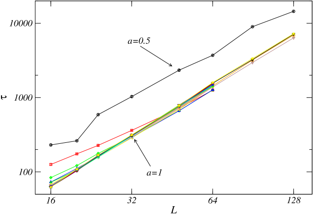
Figure 11: Auto-correlation time $\tau$ on the critical line as a function of the lattice size $L$. The different curves correspond to different values of the parameter $a$.

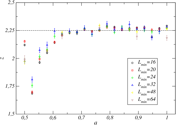
Figure 12: Dynamical exponent $z$ obtained by interpolation of the auto-correlation time $\tau$. The different symbols correspond to exponents obtained by power-law interpolation with taking into account lattice size $L\geq L_{\rm min}$ only.

4 Aging

4.1 Numerical methodology

The system is now considered out of the stationary regime, that is, in the transient regime occurring before it reaches the stationary state. It is initially prepared in a random state, i.e., in the paramagnetic phase. At time $t=0$, it is ”quenched” to some values of $a$ and $b$. A number $t_{f}$ of Monte Carlo steps are then performed. The numerical experiment is repeated $n_{\rm conf}$ times. In this section, $\overline{X(t)}$ means an average of the observable $X$ at time $t$ over all these $n_{\rm conf}$ histories.

Motivated by the fact that it is possible to couple a magnetic field to any of the $q$ spin states and thus to define $q$ possible response functions, we will now define $q$ spin-spin autocorrelation functions as

$$C_{\sigma}(i;t,s)=\overline{m_{\sigma}(i;t)m_{\sigma}(i;s)},$$ (28)

where $m_{\sigma}(i;t)=(q\delta_{\sigma_{i}(t),\sigma}-1)/(q-1)$ is the local magnetization at time $t$ on site $i$. Since translation invariance is expected, we can average over the lattice to get a more stable estimate:

$$C_{\sigma}(t,s)={1\over N}\sum_{i}C_{\sigma}(i;t,s).$$ (29)

Finally, all Potts states being equivalent, one can define a spin-spin autocorrelation function as

$$C(t,s)=\sum_{\sigma=1}^{q}C_{\sigma}(t,s).$$ (30)

One can easily check that these definitions lead simply to

$$C(t,s)=\frac{1}{(q-1)^{2}}\left(\frac{q^{2}}{N}\sum_{i}\overline{\delta_{\sigma_{i}(t),\sigma_{i}(s)}}-q\right).$$ (31)

For uncorrelated spins at times $t$ and $s$, this autocorrelation function vanishes.

A magnetic field $h$ is coupled to a particular value $\sigma_{h}$ among the $q$ Potts states by modifying the transition rates by a multiplicative factor [16, 19, 20]:

$$w(\sigma_{i}\rightarrow\sigma_{i}^{\prime})=w_{0}(\sigma_{i}\rightarrow\sigma_{i}^{\prime})e^{-h\delta_{\sigma_{i},\sigma_{h}}}.$$ (32)

The magnetic field is branched only during one MCS, at time $s$. The linear response of magnetization to this field is defined as

$$R_{\sigma}(i;t,s)={\delta\overline{m_{\sigma_{h}}(i;t)}\over\delta h(s)},$$ (33)

where again $m_{\sigma}(i;t)=(q\delta_{\sigma_{i}(t),\sigma}-1)/(q-1)$ is the local magnetization. The numerical method used to calculate this response is presented in the Appendix. As for the correlation function, the response can be averaged over the lattice and then the different responses can be added since all states are equivalent:

$$R(t,s)={1\over N}\sum_{\sigma_{h}=1}^{q}\sum_{i=1}^{N}R_{\sigma_{h}}(i;t,s).$$ (34)

Finally, the Fluctuation-Dissipation Ratio (FDR) is defined as

$$X(t,s)={R(t,s)\over\partial_{s}C(t,s)}\simeq{R(t,s)\over C(t,s+1)-C(t,s)}.$$ (35)

We have also considered global quantities: the magnetization-magnetization correlation function

$$C_{M}(t,s)=\overline{M(t)M(s)}={1\over N^{2}}\sum_{i,j}\overline{m_{\sigma}(i;t)m_{\sigma}(j;s)},$$ (36)

and the response to global magnetic field

$$R_{M}(t,s)={\delta\overline{M(t)}\over\delta H(s)}={1\over N^{2}}\sum_{i,j}R_{i,j}(t,s),$$ (37)

as well as the associated Fluctuation-Dissipation Ratio.

4.2 Aging at the voter point

We consider first a quench at the point $a=1/2$ and $b=1$ belonging to the voter universality class. As will be shown in the following, the theoretical predictions given in Ref. [16] are well reproduced by the numerical data. The spin-spin two-time auto-correlation function $C(t,s)$ is expected to behave as

$$C(t,s)\sim{s\over(t-s)\ln s}.$$ (38)

We used a lattice size $L=192$, a final time $t_{f}=1000$ and observables have been averaged over $n_{\rm conf}=10^{6}$ histories of the system. As shown on figure 13, the data indeed tend toward the theoretical prediction when $t$ and $s$ are sufficiently large. The exponent $\lambda/z$ is thus 1. The Fluctuation-Dissipation Ratio $X(t,s)$ is presented on figure 14. Its asymptotic limit is compatible with the theoretical prediction $X_{\infty}=1/2$. Interestingly, the FDR associated to the global magnetization reaches a plateau at the value $X_{\infty}$ almost immediately. Even though, this quantity is noisier, it can be used to estimate $X_{\infty}$ at very short times at the price of a higher statistics.

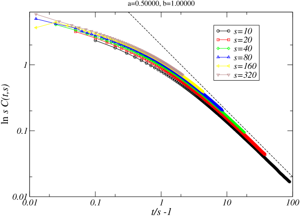
Figure 13: Scaling function $\ln s\ \!C(t,s)$ versus $t/s-1$ at the point $a=1/2$ and $b=1$ belonging to the voter universality class. The dashed line is $2/(t/s-1)$.

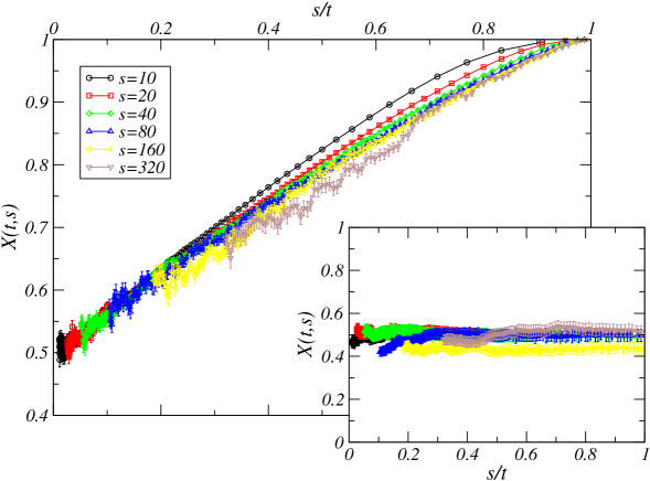
Figure 14: Fluctuation-Dissipation Ratio $X(t,s)$ versus $s/t$ at the point $a=1/2$ and $b=1$ belonging to the voter universality class. In the inset, the FDR associated to the global magnetization is plotted.

4.3 Aging on the critical line

We studied the aging at several points on the critical line. Because of the cross-over with the voter fixed point, several lattices sizes, $L=64$, $L=128$ and $L=256$, were considered.

The spin-spin correlation function is expected to behave asymptotically as [21, 22]

$$C(t,s)\sim s^{-a_{c}}\left(\frac{t}{s}\right)^{-\lambda/z},$$ (39)

where $a_{c}=2\beta/\nu z$. The scaling form is tested by plotting the scaling function $s^{a_{c}}C(t,s)$ with respect to $t/s$. The collapse of the curves for different waiting times is obtained (see figure 15) but the exponent $a_{c}$ leading to this collapse tends to grow along the critical line: from the expected value ${2\beta/\nu z}\simeq 0.11$ close to the voter point to $0.2$ at $a=1$. This indicates that for the largest values of $s$, the asymptotic regime $C(s,s)\sim s^{-a_{c}}$ is not reached yet and corrections to this dominant behavior cannot be neglected. Nevertheless, the resulting scaling function $s^{a_{c}}C(t,s)$ appears very similar along the critical line and an algebraic decay with $t$ is observed for all waiting times. This provides further evidence of a unique universality class along the critical line. The exponent $\lambda/z$ is obtained by power-law interpolation of $C(t,s)$ with the time $t$. For each value of the waiting time $s$, the data are interpolated within a sliding window $[t/s,t_{f}/s]$. The effective exponents are represented as a function of $s/t$ in figure 16. The asymptotic value is read at the intercept with the $y$-axis while the small slope that can be observed comes from the corrections to the behavior $(t/s)^{-\lambda/z}$. We finally extrapolated the effective exponents and obtained $\lambda/z\simeq 0.806(5)$, $0.817(4)$, $0.820(4)$ and $0.818(3)$ for $a=0.63158$, $0.76316$, $0.89474$, and $1$, respectively. These values should be compared with the values $0.828(2)$ [17] and $0.844(19)$ [23] obtained in the case of the pure three-state Potts model.

 

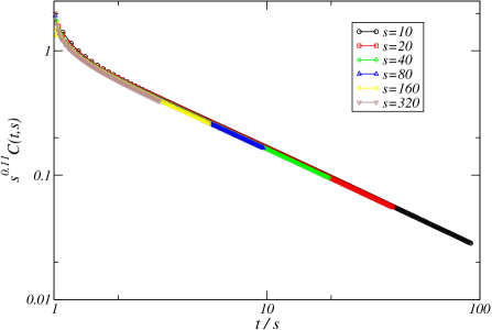
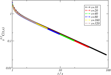
Figure 15: Scaling function $s^{a_{c}}C(t,s)$ with respect to $t/s$ for two points on the critical line ($a=0.63158$ on the left and $a=1$ on the right). The different curves correspond to different waiting times $s$. The lattice size is $L=256$.

  

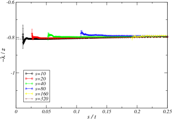
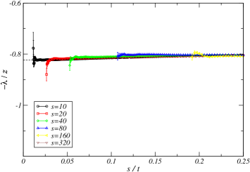
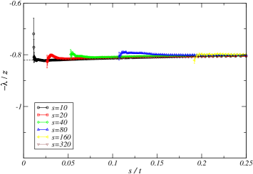
Figure 16: Effective exponent $-\lambda/z$ as a function of the smallest bound $t/s$ of the interpolation window of $C(t,s)$. From left to right, $a=0.63158$, $0.89474$ and $a=1$. The different curves correspond to different waiting times $s$. The dashed line is the power-law regression of the data.

 

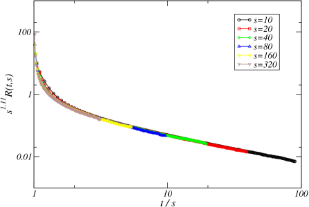
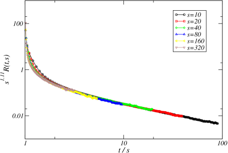
Figure 17: Scaling function $s^{1+a_{c}}R(t,s)$ with respect to $t/s$ for two points on the critical line ($a=0.63158$ on the left and $a=1$ on the right). The different curves correspond to different waiting times $s$. The lattice size is $L=256$.

The same exponents can be obtained from the scaling of the response function $R(t,s)$. In contradistinction to the correlation function, the collapse of the scaling function $s^{1+a_{c}}R(t,s)$ is obtained with the expected value $a_{c}=2\beta/\nu z$ all along the critical line (see figure 17). The response function seems to be affected by weaker corrections than the correlation function. However, the response is noisier than $C(t,s)$ and the effective exponents $\lambda/z$ obtained from a power-law interpolation of the decay of $R(t,s)$ with $t$ are compatible but much less accurate than the exponents computed from $C(t,s)$.

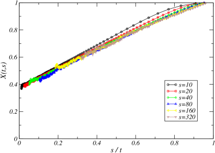
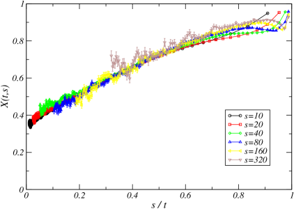
Figure 18: Fluctuation-Dissipation Ratio $X(t,s)$ versus $s/t$ for $a=0.63158$ (left) and $a=1$ (right). The different curves correspond to different waiting times $s$.

From the response function and the derivative of the correlation function, the Fluctuation-Dissipation Ratio $X(t,s)$ was computed. The asymptotic value $X_{\infty}$ is expected to be universal. As the parameter $a$ is increased, larger and larger fluctuations are observed (figure 18). The asymptotic value seems to be a bit lower, at least for the small waiting times, than the value $X_{\infty}\simeq 0.406$ for the three-state Potts model [23]. It remains nevertheless always compatible within statistical fluctuations.

4.4 Aging in the ferromagnetic phase

The system is now prepared in a random state and quenched in the ferromagnetic phase at the point of parameters $a=0.9$ and $b=0.95$. The auto-correlation exponent $\lambda/z$ is extracted from the decay of the autocorrelation function $C(t,s)\sim M^{2}(s)t^{-\lambda/z}$. The corrections to the dominant behavior appear to be very strong. Like on the critical line, we have computed an effective exponent $\lambda/z$ by power-law interpolation of $C(t,s)$ within a sliding window $[t/s,t_{f}/s]$. The asymptotic value is expected to be recovered when $t$ goes to $t_{f}$. It turns out that the effective exponent behaves linearly with $(s/t)^{1/4}$ for sufficiently small values of $s/t$ (figure 19). This simply means that the autocorrelation function behaves as $C(t,s)\sim t^{-\lambda/z}[1+at^{-1/4}+\ldots]$. The exponent $\lambda/z$ is extrapolated by a simple linear fit of the data in the linear regime. The value $0.595(15)$ obtained for the three-state Potts model [24] is nicely reproduced for the largest waiting times: we get $0.605(3)$ for $s=80$, $0.599(3)$ for $s=160$ and $0.601(3)$ for $s=320$. These exponents are remarkably stable when the interpolation window is changed (at least when remaining in the linear regime). In the ferromagnetic phase, the Fluctuation-Dissipation Ratio $X(t,s)$ is expected to decay as $s^{-a}$ to zero. The numerical data confirms this prediction (figure 20) with the predicted value $a=1/2$.

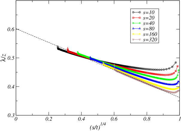
Figure 19: Effective exponent $\lambda/z$ obtained by a power-law interpolation of the autocorrelation function in a shrinking window $[t;t_{f}]$ and plotted with respect to $(s/t)^{1/4}$. The dashed line is the linear interpolation of the $s=320$ curve.

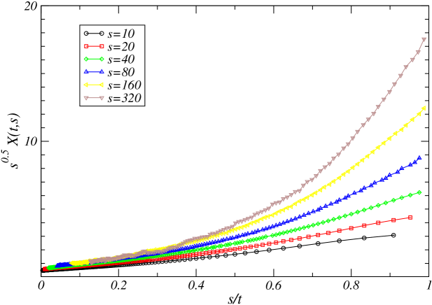
Figure 20: Fluctuation-Dissipation Ratio $X(t,s)$ with respect to $s/t$ when the system is quenched in the ferromagnetic phase.

5 Conclusions

We have shown that the class of non-equilibrium three-state lattice models with $Z_{3}$ symmetry that we introduced in this paper displays a phase diagram consisting of a critical line belonging in the three-state Potts model universality class and of an ending point in the voter class. The simulations for this model are difficult because of the absence of cluster algorithm that would reduce the critical slowing down and because the critical line cannot be determined by self-duality arguments. We thus obtain less accurate estimates of the critical exponents than for the usual equilibrium three-state Potts model. Therefore, we essentially limited ourselves to check the compatibility with the theoretical predictions, namely, that non-equilibrium models with the symmetry of the Potts model belongs to the universality class of the equilibrium Potts model along the critical line. The cross-over with the point in the voter universality class remains weak in the Finite-Size Scaling of the averages in the stationary state but turns out to be very strong in the dependence of the scaling function with $b$. In a second step, the model was studied in the aging regime after a sudden quench either on the critical line or in the ferromagnetic phase. The results are again compatible with either the theoretical predictions for the voter model or the numerical estimates for the Potts model. Surprisingly, the corrections are stronger in the ferromagnetic phase than on the critical line.

Appendix: Numerical estimation of the response

Several different methods for the calculation of the response function without applying any magnetic field have been proposed. Our method is based on [25] and was adapted to our more general transition rates. For completeness, it is presented in the following.

Preliminaries on master equations

The dynamics is a Markovian process governed by the master equation

$$\partial_{t}{\cal P}(\sigma,t)=\sum_{\sigma^{\prime}}\big{[}{\cal P}(\sigma^{\prime},t)W(\sigma^{\prime}\rightarrow\sigma)-{\cal P}(\sigma,t)W(\sigma\rightarrow\sigma^{\prime})\big{]},$$ (40)

where $\sigma$ denotes the vector whose components are the spin variables $\{\sigma_{i}\}$ attached to the sites of the lattice. The transition rates $W(\sigma\rightarrow\sigma^{\prime})$ do not appear in the equation when $\sigma=\sigma^{\prime}$ so they are free to take any value. In discrete time (Monte Carlo simulation), this master equation is replaced by

$${\cal P}(\sigma,t+1)={\cal P}(\sigma,t)+\sum_{\sigma^{\prime}}\big{[}{\cal P}(\sigma^{\prime},t)W(\sigma^{\prime}\rightarrow\sigma)-{\cal P}(\sigma,t)W(\sigma\rightarrow\sigma^{\prime})\big{]},$$ (41)

which can be written as

$${\cal P}(\sigma,t+1)=\sum_{\sigma^{\prime}}{\cal P}(\sigma^{\prime},t)\omega(\sigma^{\prime}\rightarrow\sigma),$$ (42)

where we have introduced the quantity

$$\omega(\sigma^{\prime}\rightarrow\sigma)=\big{[}1-\sum_{\sigma^{\prime\prime}}W(\sigma\rightarrow\sigma^{\prime\prime})\big{]}\delta_{\sigma,\sigma^{\prime}}+W(\sigma^{\prime}\rightarrow\sigma),$$ (43)

that can be interpreted as the conditional probability for the system to undergo a transition from $\sigma^{\prime}$ to $\sigma$ if $\sigma\neq\sigma^{\prime}$ or the probability to stay in the same state if $\sigma=\sigma^{\prime}$. It is easily shown that

$$\sum_{\sigma}\omega(\sigma^{\prime}\rightarrow\sigma)=1,$$ (44)

as required for the probability ${\cal P}(\sigma,t)$ to be normalized at any time $t$.

Response function in the general case

We are interested in the response to a magnetic field

$$R_{ij}(t,s)=\left({\partial\overline{m_{i}(t)}\over\partial h_{j}(s)}\right)_{h_{j}\rightarrow 0},$$ (45)

where $\overline{m_{i}(t)}$ is the average magnetization on site $i$ at time $t$. The response to a global magnetic field $H=\sum_{i}h_{i}$ acting on all sites is measured as

$$R(t,s)={\partial\overline{M(t)}\over\partial H(s)}=\sum_{i}{\partial\overline{m_{i}(t)}\over\partial H(s)}=\sum_{i,j}{\partial\overline{m_{i}(t)}\over\partial h_{j}(s)}=\sum_{i,j}R_{ij}(t,s).$$ (46)

To measure the linear response to a magnetic field $h_{j}$ at time $s$, the transition rates are modified between the interval of time $[s;s+1[$. This is obviously done with Glauber transition rates by introducing a Zeeman interaction in the Hamiltonian. In the present case of non-equilibrium models, that are not defined by a Hamiltonian, the perturbation should be introduced into the transition rate. We use here a prescription similar to that used for the non-equilibrium models with two states [19, 20] and which has been used in Ref. [16], namely,

$$W_{h}(\sigma\rightarrow\sigma^{\prime})=W(\sigma\rightarrow\sigma^{\prime})\,e^{-\sum_{j}h_{j}m_{j}(\sigma^{\prime})}.$$ (47)

Notice that this choice does not break the detailed balance if it was satisfied by $W(\sigma\rightarrow\sigma^{\prime})$. Other choices of perturbation include the one introduced in Ref. [26].

The average magnetization on site $i$ and time $t$ is given by

$$\overline{m_{i}(t)} = \sum_{\sigma}m_{i}(\sigma){\cal P}(\sigma,t)$$ (48)

$$= \sum_{\sigma,\sigma^{\prime}}m_{i}(\sigma){\cal P}(\sigma,t|\sigma^{\prime},s+1){\cal P}(\sigma^{\prime},s+1)$$

$$= \sum_{\sigma,\sigma^{\prime},\sigma^{\prime\prime}}m_{i}(\sigma){\cal P}(\sigma,t|\sigma^{\prime},s+1)\omega(\sigma^{\prime\prime}\rightarrow\sigma^{\prime}){\cal P}(\sigma^{\prime\prime},s).$$

When branching the magnetic field, the transition rate $\omega_{h}(\sigma^{\prime}\rightarrow\sigma)$ has to be replaced by

$$\omega_{h}(\sigma^{\prime}\rightarrow\sigma)=\Big{[}1-\sum_{\sigma^{\prime\prime}}W(\sigma\rightarrow\sigma^{\prime\prime})e^{-\sum_{j}h_{j}m_{j}(\sigma^{\prime\prime})}\Big{]}\delta_{\sigma,\sigma^{\prime}}+W(\sigma^{\prime}\rightarrow\sigma)e^{-\sum_{j}h_{j}m_{j}(\sigma)},$$ (49)

so that the average magnetization at time $t$ is perturbed by the magnetic field

$$\overline{m_{i}(t)}=\sum_{\sigma,\sigma^{\prime},\sigma^{\prime\prime}}m_{i}(\sigma){\cal P}(\sigma,t|\sigma^{\prime},s+1)\omega_{h}(\sigma^{\prime\prime}\rightarrow\sigma^{\prime}){\cal P}(\sigma^{\prime\prime},s).$$ (50)

The linear response follows:

$$R_{ij}(t,s) = \sum_{\sigma,\sigma^{\prime},\sigma^{\prime\prime}}m_{i}(\sigma){\cal P}(\sigma,t|\sigma^{\prime},s+1){\partial\omega_{h}\over\partial h_{j}}(\sigma^{\prime\prime}\rightarrow\sigma^{\prime}){\cal P}(\sigma^{\prime\prime},s)$$

$$= \sum_{\sigma,\sigma^{\prime},\sigma^{\prime\prime}}m_{i}(\sigma){\cal P}(\sigma,t|\sigma^{\prime},s+1)\Big{[}\sum_{\sigma_{3}}m_{j}(\sigma_{3})W(\sigma^{\prime}\rightarrow\sigma_{3})\Big{]}\delta_{\sigma^{\prime},\sigma^{\prime\prime}}{\cal P}(\sigma^{\prime\prime},s)$$

$$\quad-\sum_{\sigma,\sigma^{\prime},\sigma^{\prime\prime}}m_{i}(\sigma){\cal P}(\sigma,t|\sigma^{\prime},s+1)m_{j}(\sigma^{\prime})W(\sigma^{\prime\prime}\rightarrow\sigma^{\prime}){\cal P}(\sigma^{\prime\prime},s).$$

From the definition of $\omega(\sigma^{\prime\prime}\rightarrow\sigma^{\prime})$, the transition rate can be written as

$$W(\sigma^{\prime\prime}\rightarrow\sigma^{\prime})=\omega(\sigma^{\prime\prime}\rightarrow\sigma^{\prime})-\big{[}1-\sum_{\sigma_{3}}W(\sigma^{\prime}\rightarrow\sigma_{3})\big{]}\delta_{\sigma^{\prime},\sigma^{\prime\prime}}.$$ (52)

Introducing this equality into the second line of the expression of the response, one gets

$$R_{ij}(t,s) = \sum_{\sigma,\sigma^{\prime},\sigma^{\prime\prime}}m_{i}(\sigma){\cal P}(\sigma,t|\sigma^{\prime},s+1)\Big{[}m_{j}(\sigma^{\prime})$$

$$\quad+\sum_{\sigma_{3}}\big{(}m_{j}(\sigma_{3})-m_{j}(\sigma^{\prime})\big{)}W(\sigma^{\prime}\rightarrow\sigma_{3})\Big{]}\delta_{\sigma^{\prime},\sigma^{\prime\prime}}{\cal P}(\sigma^{\prime\prime},s)$$

$$\quad-\sum_{\sigma,\sigma^{\prime},\sigma^{\prime\prime}}m_{i}(\sigma){\cal P}(\sigma,t|\sigma^{\prime},s+1)m_{j}(\sigma^{\prime})\omega(\sigma^{\prime\prime}\rightarrow\sigma^{\prime}){\cal P}(\sigma^{\prime\prime},s).$$

In the second line, the sum over $\sigma^{\prime\prime}$ can be performed. It leaves a correlation function of observables measured at time $t$ and $s+1$. However, in the first line, a transition rate $\omega$ between the spin configurations at time $s$ and $s+1$ is missing to do the same thing. We thus write

$$R_{ij}(t,s) = \sum_{\sigma,\sigma^{\prime},\sigma^{\prime\prime}}m_{i}(\sigma){\cal P}(\sigma,t|\sigma^{\prime},s+1)\Big{[}m_{j}(\sigma^{\prime})+\sum_{\sigma}\big{(}m_{j}(\sigma)-m_{j}(\sigma^{\prime})\big{)}W(\sigma^{\prime}\rightarrow\sigma)\Big{]}$$

$$\hskip 113.81102pt\times{\delta_{\sigma^{\prime},\sigma^{\prime\prime}}\over\omega(\sigma^{\prime}\rightarrow\sigma^{\prime\prime})}\omega(\sigma^{\prime}\rightarrow\sigma^{\prime}){\cal P}(\sigma^{\prime\prime},s)$$

$$\quad-\sum_{\sigma,\sigma^{\prime},\sigma^{\prime\prime}}m_{i}(\sigma){\cal P}(\sigma,t|\sigma^{\prime},s+1)m_{j}(\sigma^{\prime})\omega(\sigma^{\prime\prime}\rightarrow\sigma^{\prime}){\cal P}(\sigma^{\prime\prime},s).$$

Since

$$\omega(\sigma^{\prime}\rightarrow\sigma^{\prime})=1-\sum_{\sigma}W(\sigma^{\prime}\rightarrow\sigma)+W(\sigma^{\prime}\rightarrow\sigma^{\prime}),$$ (53)

the response is finally given by the general expression

$$R_{ij}(t,s)=\overline{m_{i}(t)\Big{[}\Delta m_{j}^{\rm MF}(s)\delta_{\sigma(s),\sigma(s+1)}-m_{j}(s+1)\Big{]}},$$ (54)

where

$$\Delta m_{j}^{\rm MF}(s)={m_{j}(s)+\sum_{\sigma^{\prime}}\big{(}m_{j}(\sigma^{\prime})-m_{j}(s)\big{)}W(\sigma(s)\rightarrow\sigma^{\prime})\over W(\sigma(s)\rightarrow\sigma(s))+1-\sum_{\sigma^{\prime}}W(\sigma(s)\rightarrow\sigma^{\prime})}.$$ (55)

In the particular case where the transition rates are chosen such that

$$\sum_{\sigma^{\prime}}W(\sigma\rightarrow\sigma^{\prime})=1,$$ (56)

which is the case in this work, the response reduces to

$$R_{ij}(t,s)=\overline{m_{i}(t)\Big{[}m_{j}^{\rm MF}(s)\delta_{\sigma(s),\sigma(s+1)}-m_{j}(s+1)\Big{]}},$$ (57)

where

$$m_{j}^{\rm MF}(s)=m_{j}(s)+{\sum_{\sigma^{\prime}\neq\sigma(s)}m_{j}(\sigma^{\prime})W(\sigma(s)\rightarrow\sigma^{\prime})\over W(\sigma(s)\rightarrow\sigma(s))}.$$ (58)

In the case of the Ising model with Glauber transition rates, one recovers the result of [25] up to a factor $-\beta$ due to a difference in the definition of the magnetic field. Note that is not possible to calculate the response in this way if there exists a spin configuration $\sigma$ for which $W(\sigma\rightarrow\sigma)=0$. The trick to circumvent this difficulty, is to modify the model as

$$W^{\prime}(\sigma\rightarrow\sigma^{\prime})=p\delta_{\sigma,\sigma^{\prime}}+(1-p)W(\sigma\rightarrow\sigma^{\prime}),$$ (59)

The dynamics is then simply slown down by a factor $p$.

References

References

- [1] J. L. Cardy, Scaling and Renormalization in Statistical Physics (Cambridge University Press, Cambridge, 1996).
- [2] J. Marro and R. Dickman, Nonequilibrium Phase Transitions (Cambridge University Press, Cambridge, 1999).
- [3] H. Hinrichsen, Adv. Phys. 49, 815 (2000), arXiv:cond-mat/0001070
- [4] M. Henkel, H. Hinrichsen, and S. Lübeck, Non-Equilibrium Phase Transitions, vol. 1, Absorbing Phase Transitions (Springer, 2009).
- [5] M. Henkel and M. Pleimling, Non-Equilibrium Phase Transitions, vol. 2, Ageing and Dynamical Scaling Far from Equilibrium (Springer, 2010).
- [6] F. Y. Wu, Rev. Mod. Phys. 54, 535 (1982).
- [7] A. Brunstein and T. Tomé Physica A 257, 334 (1998) ; A. Brunstein and T. Tomé, Phys. Rev. E 60, 3666 (1999) ; T. Tomé, A. Brunstein and M. J. de Oliveira, Physica A 283 107 (2000)
- [8] T. Tomé and A. Petri J. Phys. A 35, 5379 (2002), arXiv:cond-mat/0205592
- [9] M.J. de Oliveira, J.F.F. Mendes et M.A. Santos J. Phys. A 26 2317 (1993)
- [10] J-M. Drouffe et C. Godrèche J. Phys. A 32 249 (1999), arXiv:cond-mat/9807356
- [11] M.J. de Oliveira Phys. Rev. E 67 066101 (2003)
- [12] J.F.F. Mendes et M.A. Santos Phys. Rev. E 57 108 (1998) arXiv:cond-mat/9707244
- [13] T. Tomé et M.J. de Oliveira Phys. Rev. E 58 4242 (1998)
- [14] F. Sastre, I. Dornic et H. Chaté Phys. Rev. Lett. 91 267205 (2003), arXiv:cond-mat/0308178
- [15] J. Salas and A. D. Sokal, J. Stat. Phys. 87, 1 (1997), arXiv: hep-lat/9605018
- [16] M. O. Hase, T. Tomé, and M. J. de Oliveira Phys. Rev. E 82, 011133 (2010), arXiv:1002.1842
- [17] L. Schuelke and B. Zheng, Phys. Lett. A 204, 295 (1995), arXiv:cond-mat/9510109
- [18] R. da Silva, N. A. Alves, and J. R. Drugowich de Felício Phys. Lett. A 298, 325 (2002), arXiv:cond-mat/0111288
- [19] M. Hase, S. R. Salinas, T. Tomé and M. J. de Oliveira, Phys. Rev. E 73, 056117 (2006), arXiv:cond-mat/0602318
- [20] M. J. de Oliveira, Phys. Rev. E 76, 011114 (2007).
- [21] H.K. Janssen, B. Schaub and B. Schmittmann, Z. Phys. B 73 539 (1989)
- [22] Godrèche C and Luck J M, J. Phys. Cond. Matter 14 1589 (2002) arXiv:cond-mat/0109212
- [23] C. Chatelain, J. Stat. Mech.: Theor. Exp. P06006 (2004) arXiv:cond-mat/0404017
- [24] E. Lorenz and W. Janke, Eur. Phys. Lett. 77 10003 (2007).
- [25] C. Chatelain, J. Phys. A 36, 10739 (2003), arXiv:cond-mat/0303545
- [26] N. Andrenacci, F. Corberi, and E. Lippiello, Phys. Rev. E 73, 046124 (2006). arXiv:cond-mat/0603137