Curve Reconstruction in Riemannian Manifolds:
Ordering Motion Frames

Abstract

In this article we extend the computational geometric curve reconstruction approach to curves in Riemannian manifolds. We prove that the minimal spanning tree, given a sufficiently dense sample set of a curve, correctly reconstructs the smooth arcs and further closed and simple curves in Riemannian manifolds. The proof is based on the behaviour of the curve segment inside the tubular neighbourhood of the curve. To take care of the local topological changes of the manifold, the tubular neighbourhood is constructed in consideration with the injectivity radius of the underlying Riemannian manifold. We also present examples of successfully reconstructed curves and show applications of curve reconstruction to ordering motion frames.

1 Introduction

The curve reconstruction problem can be thought of as connect the dots. The idea is quite similar to Nyquist’s sampling theorem for band limited signals in signal processing. The only difference is in terms of ordering the sample. Unlike in the latter case, the ordering is lost when we have a sample of data points on a curve. The problem of reconstruction thus demands first to establish a proper sampling criterion for the curve, next a provable ordering algorithm based on the sampling criterion to give a polygonal approximation of the original curve, and finaly an interpolating scheme to smooth out the corners. The nature of problem to be dealt with in this article corresponds to the first. Suppose an object in $\mathbb{R}^{3}$ is in motion and we have captured some frames of this motion. But these frames are jumbled up, i.e. the ordering is lost. Reconstruct the original motion given that the frames captured form a dense sample set.

We extend the ideas of curve reconstruction in Euclidean space - $\mathbb{R}^{n}$ to Riemannian manifolds. In this article we make an attempt to extend the computational geometric curve reconstruction approach to curved spaces.

It turns out that the riemannian manifold we are interested in, $SE(3)$, is endowed with an additional structure of the group, which makes Riemannian manifold into a Lie Group. It is a well studied object in physics and mathematics. Although no bi-invariant metric exist on $SE(3)$, together with the Riemannian metric defined on it the exponential map and further a left invariant distance metric on $SE(3)$ is expressed in a closed form. We give examples of successfully reconstructed curves in $SE(2)$ and $SE(3)$. We also show an application of curve reconstruction in $SE(2)$ for video frame ordering. We show that for a densely sampled curves, minimal spanning tree(MST) gives a correct polygonal reconstruction of curves in Riemannian manifolds. We also interpolate the ordered point set by a partial geodesic interpolation. Further we propose to interpolate the ordered point set with de Casteljau algorithm assuming the boundary conditions are known.

2 Background

We begin with a quick review of curve reconstruction in the plane, keeping the notations and definitions as general as possible. A curve, for our purpose, is the set of image points of a function $\gamma:[0,1]\to\mathcal{M}$. More specifically looking at the application at hand, we restrict $\mathcal{M}$ to be a differentiable manifold. We denote a curve by a symbol $\mathcal{C}$. Since it is an image of a compact interval, $\mathcal{C}$ is a one dimensional compact manifold. It is also differentiable if $\gamma$ is differentiable. $\mathcal{C}$ is smooth if $\gamma$ is smooth. A subclass of curves those are smooth and simple is of vital importance in pattern recognition, graphics, image processing and computer vision.

If $\mathcal{M}$ is $\mathbb{R}^{2}$ then the problem is of reconstructing curves in a plane and $\mathcal{C}$ is planar. $\mathbb{R}^{2}$ along with the standard Euclidean distance metric becomes a metric space. Naturally the question arise, is it always possible to have a finite sample set $\mathcal{S}\subset\mathcal{C}$ which captures everything about $\mathcal{C}$? The answer lies in the fact that $\mathcal{C}$ is compact and $\gamma$ is smooth. To appreciate it more clearly let us look at a definition of an $\varepsilon$-net. If $\varepsilon>0$ is given, a subset $\mathcal{S}$ of $\mathcal{C}$ is called an $\varepsilon$-net if $\mathcal{S}$ is finite and its $\mathcal{C}\subset\cup_{s\in\mathcal{S}}B_{\varepsilon}(s)$, where $B_{\varepsilon}(s)$ is an open ball in $\mathcal{M}$ with radius $\varepsilon$. In other words if $\mathcal{S}$ is finite and its points are scattered through $\mathcal{C}$ in such a way that each point of $\mathcal{C}$ is distant by less than $\varepsilon$ from at least one point of $\mathcal{S}$. Since $\mathcal{C}$ is compact every cover will have a finite sub-cover, which shows a possibility of a finite representative sample set of $\mathcal{C}$. The concept of $\varepsilon$-net captures the idea of sampling criterion very well.

In [1], based on the uniform sampling criterion an Euclidean MST is suggested for the reconstruction. In the initial phase of the development, uniform sampling criterion was the bottleneck. The first breakthrough came with the non-uniform sampling criterion suggested based on the local feature size by [2]. Unlike the uniform sampling it samples the curve more where the details are more. Non-uniform sampling is based on the medial axis of the curve. The medial axis of a curve $\mathcal{C}$ is closure of the set of points in $\mathcal{M}$ which have two or more closest points in $\mathcal{C}$. A simple closed curve in a plane divides the plane into two disjoint regions. Medial axis can be thought of as the union of disjoint skeletons of the regions divided by the curve. The Local feature size, $f(p)$, of a point $p\in\mathcal{C}$ is defined as the Euclidean distance from $p$ to the closest point $m$ on the medial axis.

$\mathcal{C}$ is $\varepsilon$-sampled by a set of sample points $\mathcal{S}$ if every $p\in\mathcal{C}$ is within distance $\varepsilon\cdot f(p)$ of a sample $s\in\mathcal{S}$. The algorithm suggested in [2] works based on voronoi and its dual delaunay triangulation. All delaunay based approaches can be put under a single formalism, the restricted delaunay complex, as shown in [3]. Every approach is similar in construction and differs only at how it restricts the delaunay complex. The crust [2] and further improvements NN-crust [4] can handle smooth curves. In some cases [4] it is possible to tackle the curves with boundaries and also curves in $\mathbb{R}^{d}$, $d$-dimensional euclidean space. The CRUST and NN-CRUST assume that the sample $\mathcal{S}$ is derived from a smooth curve $\mathcal{C}$. The question of reconstructing non smooth cuves have also been studied. An extensive experimentation with various curve reconstruction algorithms is carried out in [5]. In [6] an extension of NN-CRUST to $\mathbb{R}^{d}$ is presented. Which opens up possibilities of extending the existing delaunay based reconstruction algorithms to higher dimensional euclidean spaces. We show an example of a curve in $SE(2)$ reconstructed by NN-CRUST.

2.1 Organization of the article

In this paper, we pose the problem of curve reconstruction in higher dimensional curved spaces. To author’s knowledge there are no reports of efforts made in this direction. We pose the problem as follows. Let $\mathcal{M}$ be a riemannian manifold. $\mathcal{C}:[0,1]\to\mathcal{M}$ is a smooth, closed and simple curve. Given a finite sample $\mathcal{S}\subset\mathcal{C}$ reconstruct the $\mathcal{C}$. Problem involves defining the appropriate $\mathcal{S}$, suggesting a provable algorithm for geodesic polygonal approximation and an interpolation scheme.

To deal with such objects, we first examine the notion of distance on surfaces and then move on to more general manifolds in section 3. We make the Riemannian manifold into a metric space with the help of the Riemennian inner product. Next we examine the metric structure of $SE(2)$ and $SE(3)$. With an example in section 4 we show that the medial axis based sampling criterion becomes meaningless in curved spaces. We define the dense sample set of a curve on Riemannian manifolds and show that in section 5 that it is possible to reorder the dense sample set. We present successfully reconstructed curves in $SE(2)$ and $SE(3)$ in section 6. And finally we conclude giving due acknowledgements.

3 Metric Structure on Riemannian Manifolds

3.1 $\mathbb{R}^{n}$ and a surface in $\mathbb{R}^{3}$

A curve in space and a curve on the surface are two different entities. $\mathbb{R}^{n}$ can be thought of as a Riemannian manifold with the usual vector inner product as the Riemannian metric. The tangent space at a point of $\mathbb{R}^{n}$ is also an $n$-dimensional vector space. With the help of the vector inner product the length of the curve $x:[0,1]\to\mathbb{R}^{n}$ is defined as: $L(x)=\int_{0}^{1}\sqrt{\langle x^{\prime}(t),x^{\prime}(t)\rangle}dt$. It turns out that the minimum length curve between two points in the Euclidean space is a straight line segment connecting them. So the distance between two points in $\mathbb{R}^{n}$ is given by $d(x,y)=\sqrt{\sum_{i=1}^{n}(x_{i}-y_{i})^{2}}$. With this as a metric $(\mathbb{R}^{n},d)$ is a metric space.

Now let us look at a two dimensional surface $\mathcal{M}$ embedded in $\mathbb{R}^{3}$. Two dimensions here indicate that each point $p\in\mathcal{M}$ has a neighbourhood homeomorphic to a subset of $\mathbb{R}^{2}$. In other words, if we associate with each point $p\in\mathcal{M}$ a tangent space $T_{p}\mathcal{M}$ then the dimension of $T_{p}\mathcal{M}$ is two , i.e. two linearly independent vectors are required to span $T_{p}\mathcal{M}$. It is now this tangent space and the basis vectors of this space which decide the Riemannian metric for a given surface. Let us consider a surface patch $x(u,v)\subset\mathbb{R}^{3}$ parametrized by $(u,v)\in\mathcal{U}\subset\mathbb{R}^{2}$. In this case $x$ is our manifold $\mathcal{M}$. Riemannian metric is defined as:

$$g_{ij}=\left[\begin{array}[]{cc}E=\langle x_{u},x_{u}\rangle&F=\langle x_{u},x_{v}\rangle\\ F=\langle x_{v},x_{u}\rangle&G=\langle x_{v},x_{v}\rangle\end{array}\right]$$ (1)

where $x_{u}$ and $x_{v}$ are partial derivatives of $x(u,v)$ w.r.t. $u$ and $v$ respectively. Any vector in $T_{p}\mathcal{M}$ can be expressed in terms of these basis vectors $x_{u}$ and $x_{v}$. The inner product for vectors $x_{1},x_{2}\in T_{p}\mathcal{M}$ is given by $\langle x_{1},x_{2}\rangle_{g}=x_{1}^{T}g_{ij}x_{2}$, where $x_{1}$ and $x_{2}$ are column vectors. Given a curve $\gamma(t)\in\mathcal{M}$, the length of the curve is defined as :

$$L(\gamma)=\int_{0}^{1}\sqrt{\langle\gamma^{\prime}(t),\gamma^{\prime}(t)\rangle_{g}}dt$$ (2)

Given $p,q\in\mathcal{M}$, let $\gamma$ be a curve lying in $\mathcal{M}$ with $p,q$ as end points. Then

$$d(p,q)=\inf L(\gamma)$$ (3)

is a valid metric on $\mathcal{M}$. A $\gamma^{*}$ for which the distance between two points is minimized is called a geodesic curve on the manifold $\mathcal{M}$. As we will see in the following example, even for a simple looking parametrized surface finding a closed form expression for the geodesic curve is difficult. In practice, $\gamma^{*}$ is obtained by numerical approximations[8].

Example 1.

Let $x(u,v)=(u,v,u\cdot v)$ which leads to $x_{u}=(1,0,v)$, $x_{v}=(0,1,u)$ and $E=1+v^{2}$, $F=u\cdot v$ and $G=1+u^{2}$. A curve in $x(u,v)$ is, $\gamma(t)=x(u(t),v(t))=(u(t),v(t),u(t)\cdot v(t))$. The length of the curve $\gamma(t)$, $t\in[t_{0},t_{1}]$ is $\int_{t_{0}}^{t_{1}}\sqrt{Eu^{\prime 2}+2\cdot F\cdot u^{\prime}\cdot v^{\prime}+Gv^{\prime 2}}dt$, where $u^{\prime}$ and $v^{\prime}$ are $du/dt$ and $dv/dt$ respectively.

If we try to minimize the length function by Euler-Lagrange minimization we get for each of the co-ordinates a second order ordinary non-linear differential equation to solve. In this example these equations are:

$$\frac{d^{2}u}{dt^{2}}+2\frac{v}{1+u^{2}+v^{2}}\frac{du}{dt}\frac{dv}{dt}=0$$ (4)

$$\frac{d^{2}v}{dt^{2}}+2\frac{u}{1+u^{2}+v^{2}}\frac{du}{dt}\frac{dv}{dt}=0$$ (5)

Let the boundary points, the points between which we are trying to find the geodesic distance, be $(1,1,1)$ and $(-1,-1,1)$. We solve the BVP for the above system of equations with matlab boundary value solver. The resultant geodesic and the initial guess are shown in the Figure.1.

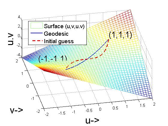
Figure 1: A bilinear surface and a geodesic

3.2 Euclidean Motion Groups

Consider an object in plane undergoing a rigid body euclidean motion. This motion can be decomposed into a rotation with respect to the center of mass of the object and a translation of the center of mass of the object. All possible configurations of an object in plane can be represented by $(\theta,u,v)$(i.e. orientation of the principle axis and the co-ordinates of the center of mass of the object), where $0\leq\theta\leq 2\pi$ and $(u,v)\in\mathbb{R}^{2}$. Let all such configurations form a set $\mathbb{S}$. It is rather intuitive to define a metric on $\mathbb{S}$ so as to compare two configurations of an object. If $A_{1}=(\theta_{1},u_{1},v_{1})$ and $A_{2}=(\theta_{2},u_{2},v_{2})$ be two configurations in $\mathbb{S}$ then it is easy to verify that

$$d(A_{1},A_{2}):=\sqrt{a(\theta_{1}-\theta_{2})^{2}+b(u_{1}-u_{2})^{2}+b(v_{1}-v_{2})^{2}}$$ (6)

is a valid metric on $\mathbb{S}$ corresponding to the riemannian inner product $\langle A_{1},A_{1}\rangle_{R}=A_{1}^{T}RA_{1}$, and $R=\left[\begin{array}[]{cc}a&0\\ 0&bI_{2}\end{array}\right]$ a positive definite matrix. Moreover for given $A_{1},A_{2}$, left composition with $A\in\mathbb{S}$, i.e $A(A_{1})=(\theta+\theta_{1},u+u_{1},v+v_{1})$, the above defined metric leads to $d(A_{1},A_{2})=d(A(A_{1}),A(A_{2}))$. Hence we have a left invariant metric defined on $\mathbb{S}$. Physical interpretation of the left invariance is the freedom in choice of the inertial reference frame. The matrix representation of $\mathbb{S}$, the euclidean motion group, is denoted by $SE(2)$. And a typical element of $SE(2)$ is made up of a rotation matrix and a translational vector. Correspondence between $\mathbb{S}$ and $SE(2)$ is given by

$$(\theta,u,v)\Leftrightarrow\left[\begin{array}[]{ccc}\cos{\theta}&\sin{\theta}&u\\ -\sin{\theta}&\cos{\theta}&v\\ 0&0&1\end{array}\right]$$

A typical curve between two configurations in $SE(2)$ and the geodesic segment from $A_{1}$ to $A_{2}$ are show in Fig.2.

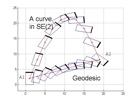
Figure 2: Comparision of a curve and a geodesic in $SE(2)$ between two configurations $A_{1}$ and $A_{2}$.

$SE(2)$ is explored in the domain of image processing for segmentation in object tracking where one is interested in constrained evolution of the curve under the action of $SE(2)$, a lie group.

In general the group of rigid body motions in $\mathbb{R}^{n}$ is the semi-direct product [9] of the special orthogonal group with $\mathbb{R}^{n}$ itself.

$$SE(n)=SO(n)\ltimes\mathbb{R}^{n}$$

Unlike $\mathbb{R}^{2}$ the rotations in $\mathbb{R}^{3}$ are not commutative. And that reflects in the group composition of $SO(3)$, $R_{1}R_{2}\neq R_{2}R_{1}$, $R_{1},R_{2}\in SO(3)$. The product of two rigid body motions $(R_{1},d_{1}),(R_{2},d_{2})\in SE(3)$ is given by $(R_{2},d_{2})(R_{1},d_{1})=(R_{2}R_{1},R_{2}d_{1}+d_{2})$. The matrix representation of elements of $SE(3)$

$$SE(3)=\{A|A=\left[\begin{array}[]{cc}R&d\\ 0&1\end{array}\right],R\in SO(3),d\in\mathbb{R}^{3}\}$$ (7)

The tangent space at the group identity in $SO(3)$ and $SE(3)$ are the lie algebras $so(3)$ and $se(3)$ respectively.

$$so(3)=\{[\omega]|[\omega]\in\mathbb{R}^{3\times 3},[\omega]^{T}=-[\omega]\},$$ (8)

$$se(3)=\{S=\left[\begin{array}[]{cc}[\omega]&v\\ 0&0\end{array}\right],[\omega]\in so(3),v\in\mathbb{R}^{3}\}$$ (11)

Where $[\omega]$ is a skew symmetric matrix [7] corresponding to the vector $\omega=[\omega_{x},\omega_{y},\omega_{z}]\in\mathbb{R}^{3}$. The $||\omega||$ gives the amount of rotation with respect to the unit vector along $\omega$. The exponential map is a diffeomorphism [10] connecting the lie algebra to the lie group. The $\exp:se(3)\to SE(3)$ is given by the usual matrix exponential as $\exp(S)=\sum_{n=0}^{\infty}\frac{S^{n}}{n!}$.

Consider a rigid body moving in free space. We fix any inertial reference frame $\{B\}$ at $o$ and a frame $\{E\}$ to the body at some point $o^{\prime}$ of the body as shown in Fig.3. At each instance the configuration of the rigid body is described via a transformation matrix, $A\in SE(3)$, corresponding to the displacement from frame $\{B\}$ to frame $\{E\}$.

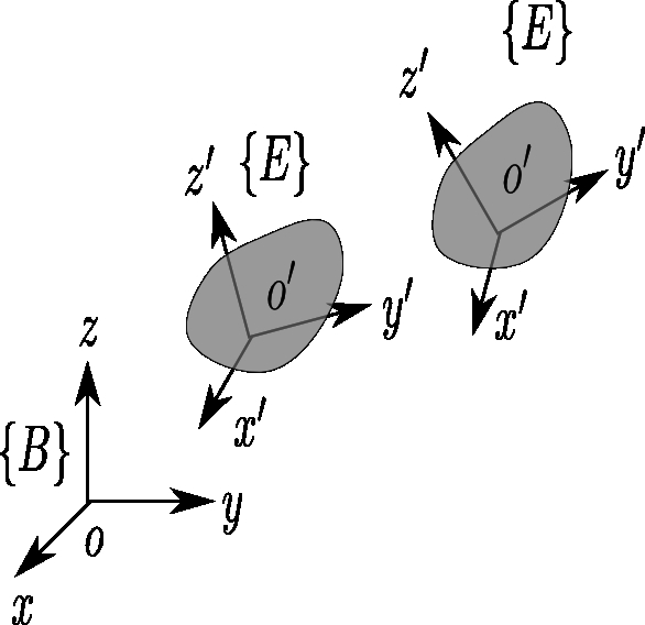
Figure 3: Inertial frame $\{B\}$ and body fixed frames $\{E\}$

So a rigid body motion becomes a curve in $SE(3)$, let $A(t)$ be such a curve given by $A(t):[-c,c]\to SE(3),A(t)=\left[\begin{array}[]{cc}R(t)&d(t)\\ 0&1\end{array}\right]$. The lie algebra element $S(t)\in se(3)$ can be identified with the tangent vector $A^{\prime}(t)$ at an arbitrary t by:

$$S(t)=A^{-1}(t)A^{\prime}(t)=\left[\begin{array}[]{cc}[\omega](t)&v(t)\\ 0&0\end{array}\right]$$ (12)

The $\omega$ physically corresponds to the angular velocity of the body, while $v$ is the linear velocity of the origin $O^{\prime}$. Let us assign a riemannian metric $g=\left[\begin{array}[]{cc}\alpha I_{3}&0\\ 0&\beta I_{3}\end{array}\right]$ over $SE(3)$ as prescribed in [11]. And so for $V=(\omega,v)\in se(3)$, $\langle V,V\rangle_{g}=\alpha\omega^{T}\omega+\beta v^{T}V$. It was proved in [10] that the analytic expression for the geodesic between two configurations $A_{1}$ and $A_{2}$ in $SE(3)$, with $g$ as riemannian metric, is given by;

$$R(t)=R_{1}\exp([\omega_{0}]t)$$ (13)

$$d(t)=(d_{2}-d_{1})t+d_{1}$$ (14)

where $[\omega_{0}]=log(R_{1}^{T}R_{2})$ and $t\in[0,1]$. The path is unique for $Trace(R_{1}^{T}R_{2})\neq-1$. And the distance between two configuration in $SE(3)$ is given by

$$d(A_{1},A_{2})=\sqrt{\alpha\|\log(R_{1}^{-1}R_{2})\|^{2}+\beta\|d_{2}-d_{1}\|^{2}}.$$ (15)

All the formulas required for computing $\exp$ and $\log$ maps are given in the Appendix.A for completeness.

Example 2.

Consider two configurations $A_{1}$ and $A_{2}$, as shown in Fig.4, given by vectors $(\omega_{1},v_{1})$ and $(\omega_{2},v_{2})$ respectivel, where $\omega_{1}=\frac{\pi}{4}\left[\begin{array}[]{ccc}1&0&0\end{array}\right]$, $v_{1}=\left[\begin{array}[]{ccc}-6&0&0\end{array}\right]$, $\omega_{2}=\frac{\pi}{2}\left[\begin{array}[]{ccc}1&1&0\end{array}\right]$ and $v_{2}=\left[\begin{array}[]{ccc}0&6&2\end{array}\right]$.

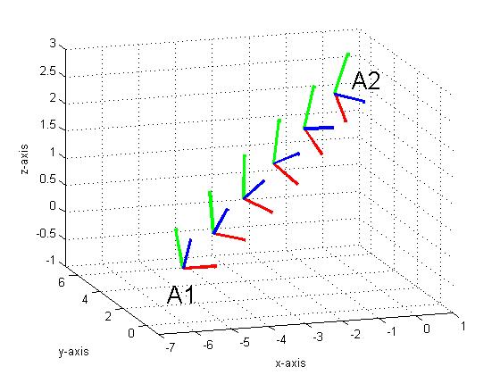
Figure 4: A geodesic between $A_{1},A_{2}\in SE(3)$.

$SE(3)$ is used extensively in robotics for path planning and motion planning of robots. It is also useful in computer vision and graphics.

Once the Riemannian metric is identified we can construct a distance metric on the manifold. With the distance metric $d(\cdot,\cdot)$(corresponding to the geodesic path) defined on the Riemannian manifold we are now ready to talk about the medial axis and the sampling criterion for a curve on the manifold.

4 Medial Axis, Dense sample and Flatness

We proceed by revisiting the definition of the medial axis stated previously. Let $\mathcal{M}$ be a Riemannian manifold and $d(\cdot,\cdot):\mathcal{M}\times\mathcal{M}\to\mathbb{R}$ be the corresponding distance metric.

Definition 1.

The medial axis $M$ of a curve $\mathcal{C}\subset\mathcal{M}$, is the closure of the set of points in $\mathcal{M}$ that have at least two closest points in $\mathcal{C}$.

Fig.5 shows examples of medial axis of closed curves on a half cylinder and in a plane.

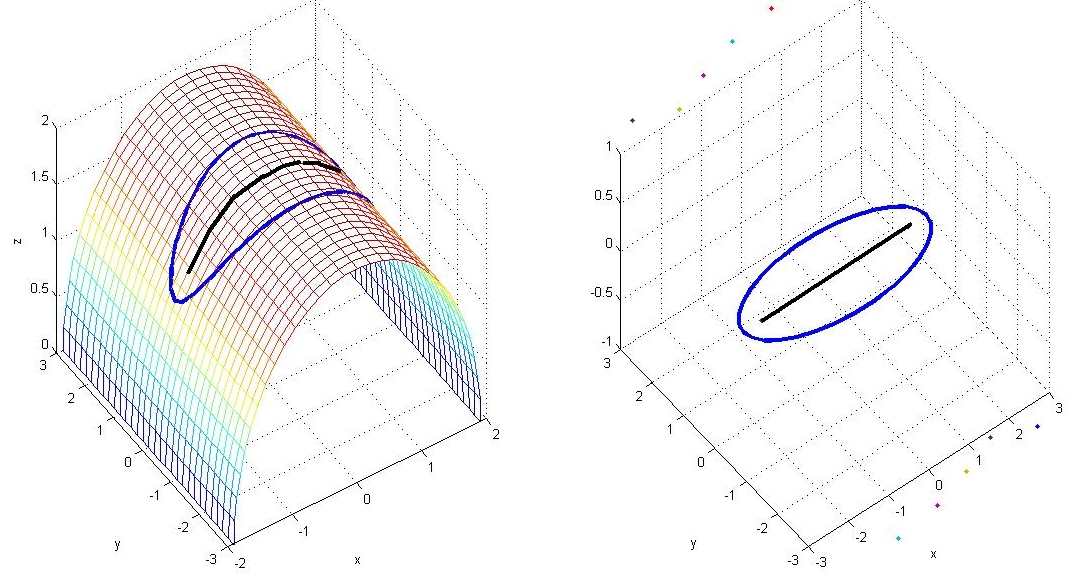
Figure 5: Medial axis of a curve on a surface and a curve in a plane

It should be noted that the medial axis, as defined above, is a subset of the underlying manifold in which the curve lies. A curve embedded in a riemannian manifold and embedded in $\mathbb{R}^{3}$ will have different medial axes. The open disc (ball) of radius $\varepsilon>0$ in $\mathcal{M}$ with $s\in\mathcal{M}$ as a center is defined as $S_{\varepsilon}(s)=\{x\in\mathcal{M}|d(s,x)<\varepsilon\}$. In the same manner $B_{\varepsilon}(s)=\{x\in\mathcal{M}|d(s,x)\leq\varepsilon\}$ is a closed disc (ball) in $\mathcal{M}$ with radius $\varepsilon$ and the center $s$. The set $\partial B_{\varepsilon}(s)=\{x\in\mathcal{M}|d(x,s)=\varepsilon\}$ is the boundary of $B_{\varepsilon}(s)$.

Definition 2.

At a point $p$ on the curve $\mathcal{C}$ the local feature size $f(p)=d(p,M)$. Where $d(p,M)=\inf\{d(p,m),\forall m\in M\}$.

The local feature size at a point on the curve captures the behaviour of the curve in the neighbourhood of that point. In practice for arbitrary curves it is difficult to identify the medial axis. Looking at the construction of the Voronoi diagram[12] for a given sample points of a curve the Voronoi vertices do capture the behaviour of the medial axis of the sampled curve. And so for a densely sampled curve the Voronoi vertices for these samples are taken to be the approximate of the medial axis of the given curve. It is computationally challenging to construct voronoi diagrams on curved spaces [13].

4.1 Dense sampling

A tubular neighbourhood for a curve in a plane is defined as the subset of the plane such that every point of the subset belongs to exactly one line segment totally contained in the subset and normal to the curve. And a disk centred on the curve contained in a tubular neighbourhood of the curve is called a tubular disk. Let us generalize this definition to curves in manifolds. We will also define the notion of a dense sample of a curve in manifold based on the tubular neighbourhood.

Definition 3.

Let $\mathcal{C}\subset\mathcal{M}$ be a smooth curve. Consider segments of geodesics that are normal to $\mathcal{C}$ and start in $\mathcal{C}$. If $\mathcal{C}$ is compact, then there exists an $\varepsilon>0$ such that no two segments of length $\varepsilon$ and starting at different points of $\mathcal{C}$ intersect [14]. The union of all such segments of length $\varepsilon$ is an open neighbourhood $T$ of $\mathcal{C}$, and is called a tubular neighbourhood of $\mathcal{C}$.

We denote the open segment with center $p\in\mathcal{C}$ and radius $\varepsilon$ in the normal geodesic segment of $\mathcal{C}$ at $p$ by $N_{\varepsilon}(p)$. Revisiting the definition of the tubular neighbourhood: the union $N_{\varepsilon}(\mathcal{C})=\cup_{p\in\mathcal{C}}N_{\varepsilon}(p)$ is called a tubular neighbourhood of radius $\varepsilon$ if it is open as a subset of $\mathcal{M}$ and the map $F:\mathcal{C}\times(-\varepsilon,\varepsilon)\to N_{\varepsilon}(\mathcal{C})$ is a diffeomorphism. This interpretation is the outcome of result from [15]. Let $\mathcal{C}\subset\mathbb{R}^{2}$, be a simple closed smooth curve. Existence of the tubular neighbourhood is evident from the compactness of the curve in $\mathbb{R}^{2}$. We show something more about the value of $\varepsilon$ in next proposition.

Proposition 1.

If $N_{\varepsilon}(\mathcal{C})$ is a tubular neighbourhood of $\mathcal{C}$ then $\varepsilon<\frac{1}{k}$. Where $k=\max{k(p)},p\in\mathcal{C}$ and $k(p)$ is the curvature of the curve at point $p$.

Proof.

Let us define a curve $\alpha(s)$ in $\mathbb{R}^{2}$ by

$$\alpha(s)=F(\mathcal{C}(s),t)=\mathcal{C}(s)+tN(\mathcal{C}(s)),$$

for a fixed $t\in(-\varepsilon,\varepsilon)$ such that $\alpha(0)=p$. $N(p)$ is the unit normal to the curve $\mathcal{C}$ at $p$. This new curve belongs to the open set $N_{\varepsilon}(\mathcal{C})$ and

$$\alpha(0)=p+tN(p)$$ (16)

$$\alpha^{\prime}(0)=\mathcal{C}^{\prime}(0)+t\mathcal{C}^{\prime\prime\prime}(0)$$ (17)

$$\alpha^{\prime}(0)=(1-tk(p))\mathcal{C}^{\prime}(0)=(dF)_{(p,t)}(\mathcal{C}^{\prime}(0))$$ (18)

Since $F:\mathcal{C}\times(-\varepsilon,\varepsilon)\to\mathbb{R}^{2}$ is a diffeomorphism when restricted to $\mathcal{C}\times(-\varepsilon,\varepsilon)$, we have that $(dF)_{(p,t)}(\mathcal{C}^{\prime}(0))$ is a non-null vector,i.e. $1-tk(p)\neq 0$. But $(-\varepsilon,\varepsilon)$ is connected and $1-tk(p)>0$ for $t=0$. Thus $1-tk(p)>0$ on $\mathcal{C}\times(-\varepsilon,\varepsilon)$. Now if we find out $k=\max k(p),p\in\mathcal{C}$ then $1-tk>0$. And we have $\varepsilon=t<\frac{1}{k}$. ∎

Definition 4.

A finite sample set $\mathcal{S}\subset\mathcal{C}$ is called a uniform $\varepsilon-$sample for some $\varepsilon>0$ if for any two consecutive sample points $r,s\in\mathcal{S}$, $r\in B_{\varepsilon}(s)$.

Definition 5.

A uniform $\varepsilon$-sample $\mathcal{S}$ of a curve $\mathcal{C}\subset\mathcal{M}$ is dense if there is a real number $\varepsilon>0$ such that $\cup_{s\in\mathcal{S}}B_{\varepsilon}(s)$,i.e. the union of the closed disks of radius $\varepsilon$ centred at the sample points $s\in\mathcal{S}$, forms a tubular neighbourhood of $C$.

Proposition 2.

For plane curves if $\varepsilon<\min_{p\in\mathcal{C}}{f(p)}$ then the uniform $\varepsilon$-sample $\mathcal{S}$ of curve $\mathcal{C}$ is a dense sample.

Proof.

By the definition of $f(p)$. ∎

Before we proceed to the main theorem we will discuss few observations in the next section. We show by an example how the medial axis based sampling fails due to the curvature of the underlying riemannian manifold. We also propose to work within the injectivity radius of the manifold to avoid such a problem.

4.2 Observations and a Counter Example

The first two observations are encouraging. And the counter example to these to in next section helps in identifying a conservative sampling condition. We know that to form a dense sample of a curve in $\mathbb{R}^{n}$ it is required to sample with the $\varepsilon_{1}<\min_{p\in\mathcal{C}}f(p)$. The curve and corresponding $\varepsilon_{1}$ is shown in Fig.6.

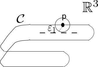
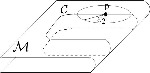
Figure 6: 6 A curve $\mathcal{C}\in\mathbb{R}^{3}$ and the part of medial axis near $p\in\mathcal{C}$. $\varepsilon_{1}$ is the distance of the point $p\in\mathcal{C}$ from the medial axis of the curve in space. 6 The same curve $\mathcal{C}$ on a surface $\mathcal{M}$ and the medial axis distance $\varepsilon_{2}$ from the point $p\in\mathcal{C}$ to the medial axis of the curve on the surface.

Whereas if the same curve is embedded in a surface, as shown Fig.6, the required $\varepsilon_{2}$ needs to be evaluated on the surface. It turns out that $\varepsilon_{2}<\varepsilon_{1}$. Let us look at another example.

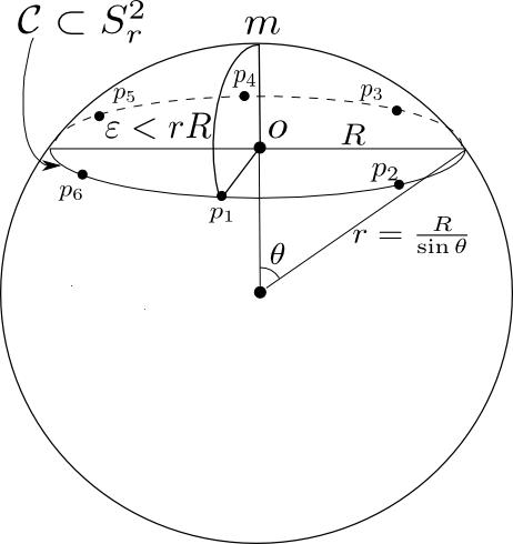
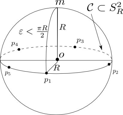
Figure 7: 7 Circle with radius R is lying in space 7 Circle resting on a sphere of radius $r=\frac{R}{\sin\theta}$ 7 Circle is the great circle the sphere of radius $R$

A circle in a $xy$-plane in $\mathbb{R}^{3}$ can be thought of as some latitude on a sphere of radius $r\geq\frac{L}{2\pi}$, where $L$ is the length of the circle. In both the cases, circle on a plane and circle on a sphere, the sampling required for correct reconstruction is different. On sphere we need less dense sample set as compared to the plane. In fact as we increase the radius $r$ we need denser and denser sample set for correct reconstruction and its limiting case, $r\to\infty$, is the plane. In $\mathbb{R}^{3}$ the usual euclidean metric is carried over to the points of the circle. In case of sphere the shortest path between two points is always along the great circle passing through these two points and the length of the segment which is shorter is the distance between two points on sphere. With this distance metric defined, sphere becomes a metric space. And the points of the circle on sphere are endowed with this metric. The points of this circle on a sphere are more structured then the points of the same circle in the space. The additional knowledge of the underlying surface adds up to the ordering relation between points of the circle. Since we know the surface we know the tangent space and that reduces the effort in ordering the sample points.

Interestingly, when generalized to the curves on manifolds, the sampling criterion based only on the medial axis becomes meaningless. As an example let us look at a circle of radius one on the surface shown in Fig.8.

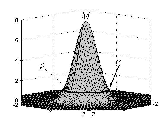
Figure 8: A circle $\mathcal{C}$ and the normal geodesic from a point $(1,0,1.0629)$ to $M$

The medial axis of the circle on the given surface is the point $M=(0,0,0)$. For any point on the circle, the distance from the medial axis turns out to be larger than the length of the circle itself. Consider the limiting case of this surface, a cylinder, suppose the circle is on the cylinder. The medial axis point does not exist.

The above phenomenon can be understood clearly if we look at the cut locus of the point $p\in\mathcal{M}$. Following can be considered as the defining property of the cut locus of a point on the manifold. If $\gamma(t_{0})$ is the cut point of $p=\gamma(0)$ along the geodesic arc $\gamma$ then either $\gamma(t_{0})$ is the first conjugate point of $\gamma(t_{0})$ or there exists a geodesic $\sigma=\gamma$ from $p$ to $\gamma(t_{0})$ such that $l(\sigma)=l(\gamma)$(lengths of $\sigma$ and $\gamma$ are equal).

For example if $\mathcal{M}$ is a sphere $S^{2}$ and $p\in S^{2}$ then the cut locus of $p$ is its antipodal point. And if we consider the sphere of radius $R$ the distance of point $p$ from its cut locus is $\pi R$. Whereas the distance of the point $p$ on the circle in Fig.7 to the medial axis $M$ is $\frac{\pi R}{2}$. Now coming back to the counter example Fig.8 we observe that the distance of the $p$ to its cut locus $d(p,C_{m}(p))$ is less then the distance to the medial axis $M$ of the circle. Where $C_{m}(p)$ is the cut locus of $p\in\mathcal{M}$.

It can be shown that if $q\in\mathcal{M}-C_{m}(p)$ there exists a unique minimizing geodesic joining $p$ and $q$. In [15]

$$i(\mathcal{M})=\inf_{p\in\mathcal{M}}d(p,C_{m}(p))$$ (19)

is called the injectivity radius of $\mathcal{M}$. So if $\varepsilon<i(\mathcal{M})$ then $\exp_{p}$ is injective on the open ball $S_{\varepsilon}(p)$.

Tubular neighbourhood for a curve is constructed by taking only the normal geodesics to the curve at a point and assuring the injectivity of the $exp_{p}$ map along these normal directions. We now propose to work inside the injectivity radius to straighten out the problem with sampling.

Proposition 3.

Let $\mathcal{C}\in\mathcal{M}$ be a smooth, simple and closed curve. If $\mathcal{S}$ is a uniform $\varepsilon$- sample of $\mathcal{C}$ then $\mathcal{S}$ is dense for $\varepsilon<\min\{\inf_{p\in\mathcal{C}}f(p),i(\mathcal{M})\}$.

4.3 Flatness of the curve inside a tubular neighbourhood

If the underlying manifold is a plane and a curve is sampled densely then based on the tubular neighbourhood it is proven, in [1], that euclidean minimal spanning tree reconstructs the sampled arc. The crucial argument for the correctness of above is the denseness of the sample. It comes from the observation that an arc does not wander too much inside a tubular disk. Which avoids the connections between the non-consecutive sample points in $\mathcal{S}$, defined as short chords.

Now we give an alternate proof of flatness of the curve segment inside a tubular neighbourhood in plane. And after that we extend the proof to curves in the riemannian manifold.

Theorem 1.

Let $p$ and $q$ be two points on an arc $\mathcal{C}\subset\mathbb{R}^{2}$ such that $q$ is inside the tubular disk $B_{\varepsilon}(p)$ centred at $p$. Then the sub arc $pq$ of $\mathcal{C}$ is completely inside $B_{pq/2}(c)$, where $c$ is the center of diameter $pq$.

Proof.

Since $q\in B_{\varepsilon}(p)$, $pq=d(p,q)\leq\varepsilon$. Now pq being a segment of an arc $\mathcal{C}$ there are three possible ways, as shown in Figure.9, in which it intersects with $B_{pq/2}(c)$.

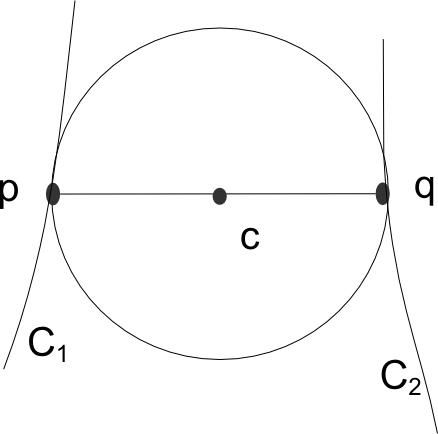
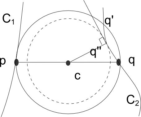
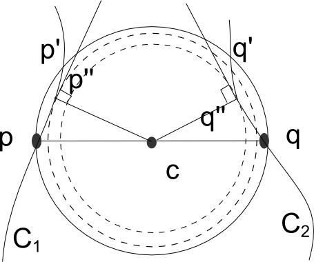
Figure 9: 9 The arc touches $B_{pq/2}(c)$ 9 The arc touches $B_{pq/2}(c)$ at $p$ and intersects its boundary at $q^{\prime}$ while passing through $q$ 9 The arc intersects boundary of $B_{pq/2}(c)$ at $p^{\prime}$ and $q^{\prime}$ while passing through $p$ and $q$ respectively

For the possibility shown in Figure.9, it is evident that center $c$ lies on two normals passing through $p$ and $q$, i.e. $c\in\overline{pq}$, since $B_{pq/2}(c)$ and $\mathcal{C}$ share common tangents at $p$ and $q$. This can not happen since $B_{pq/2}(c)\subset B_{\varepsilon}(p)$, a subset of a tubular neighbourhood.

Let us consider the case in Figure.9, arc $\mathcal{C}$ touches $B_{pq/2}(c)$ at $p$ and intersects the boundary of $B_{pq/2}(c)$ at $q$ and $q^{\prime}$. We can find out a point $q^{\prime\prime}$ on the segment $qq^{\prime}$ which is nearest to $c$. At $q^{\prime\prime}$ the circle with center $c$ and radius $d(c,q^{\prime\prime})$ shares a common tangent with $\mathcal{C}$. Hence $c$ lies on the two normals $\overline{pc}$ and $\overline{q^{\prime\prime}c}$. This can not happen inside a tubular neighbourhood.

Finally we consider the Figure.9. On segments $pp^{\prime}$ and $qq^{\prime}$ we find $p^{\prime\prime}$ and $q^{\prime\prime}$ nearest to $c$. In this case $c$ lies on $\overline{p^{\prime\prime}c}$ and $\overline{q^{\prime\prime}c}$. Since $c$ is inside tubular neighbourhood this can not happen.

So the only possibility we are left with is that the segment $pq$ of curve $\mathcal{C}$ lies entirely inside $B_{pq/2}(c)$. ∎

Theorem 2.

Let $p$ and $q$ be two points on an arc $\mathcal{C}\subset\mathcal{M}$, where $\mathcal{M}$ is any Riemannian manifold, such that $q$ is inside the tubular disk $B_{\varepsilon}(p)$ centred at $p$. Then the sub arc $pq$ of $\mathcal{C}$ is completely inside $B_{pq/2}(c)$, where $c$ is the center of diameter $pq$.

Proof.

For $\mathcal{M}:=\mathbb{R}^{n}$ we know that $\overline{cp}$, $p\in S^{n-1}$, is orthogonal to $T_{p}S^{n-1}$.

Since we are working inside a tubular neighbourhood of the curve $\mathcal{C}$, with $\varepsilon$ as prescribed in Proposition.3, $\exp:T_{p}\mathcal{M}\to\mathcal{M}$ is a diffeomorphism.

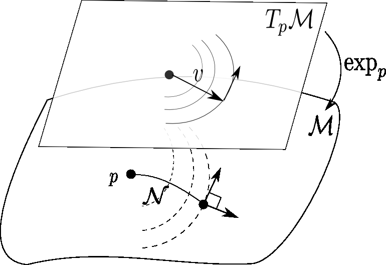
Figure 10: Tangent space of a point $p\in\mathcal{M}$ where $||v||<\varepsilon$ and the corresponding geodesic $\mathcal{N}$.

Gauss’s lemma [15] asserts that the image of a sphere of sufficiently small radius($<\varepsilon$) $T_{p}\mathcal{M}$ under the exponential map is perpendicular to all geodesics originating at $p$ Fig.10.

And the rest of the proof follows from arguments of the Theorem.1. ∎

5 Curve Reconstruction on a Riemannian manifold

5.1 Ordering

We model a curve with a graph where the vertices of the graph are the sample points and the edges indicate the order in which the vertices are connected. This also implies a geometric realization of the graph. If further we put the distance between two sample points as the edge cost, it becomes a weighted graph. A minimal spanning tree for a weighted graph is a spanning tree for which the sum of edge weights is minimal. To keep the notations consistent we define the geodesic polygonal path on riemannian manifold as the path along which every vertex(sample point) pair is connected by a geodesic segment.

Computing the minimal spanning tree use the following fundamental property, let $X\cup Y$ be a partition of the set of vertices of a connected weighted graph $G$. Then any shortest edge in $G$ connecting a vertex of $X$ and a vertex of $Y$ is an edge of a minimal spanning tree. If we use MST to model an arc, we must ensure that there are no short chords in the graph, proved in [1].

Our work focuses on closed, simple, smooth curves. We expect the MST for which every vertex has degree two. In other words the sample point has exactly two neighbours (samples) on the curve.

Theorem 3.

If $\mathcal{S}$ is a dense sample of $\mathcal{C}\subset\mathcal{M}$ then MST gives a correct geodesic polygonal reconstruction of $\mathcal{S}$. Where $\mathcal{C}$ is a smooth, closed and simple curve.

Proof.

We show that the geodesic polygonal path has no short chords. The argument is similar to the proof provided for planar case in [1]. For the completeness of the article we restate the argument here. Suppose that MST does not give a correct geodesic polygonal reconstruction of $\mathcal{S}$. It implies that there are two points in MST which are not consecutive. Let these points be $p,q\in\mathcal{S}$. Since $pq$ is a short chord there has to be at least one edge in the sub arc $pq$ which has length greater than that of $pq$. But since the sample $\mathcal{S}$ is dense, the arc $pq$ must be contained in the disc with diameter $pq$. Inside the disc there is no arc with length greater than the length of the diameter. So we have a contradiction. ∎

5.2 Interpolation

Once we have ordered the given set of points of the curve on a curved manifold the next step is to interpolate this point set to the desirable granularity. The easiest way to interpolate the points is to connect the points via straight line segments, a linear interpolation. In general for a manifold like $SE(3)$, the geodesics are the $\exp$ segments. But this scheme will not produce a differentiable curve which might be necessary for some applications. Based on the need and application one may chose the interpolation scheme. In [16] and [17] a quaternion based approach is suggested and is very useful in computer graphics and animation. Since we have represented $SE(3)$ using matrices we would rather stick to matrices. Motivated by motion planning purposes various interpolation schemes based on variational minimization techniques have been proposed and some of them turn out to be quite simple for implementations, for a broad overview one will find [18] and [19] useful. For the completeness of the reconstruction process we have used de Casteljau construction as prescribed in [20], i.e. generalizing the multilinear interpolation on $SE(3)$, a piecewise $C^{2}$ curve connecting two frames with given velocities. The advantage is that the expression is in the closed form with exponential and log maps.

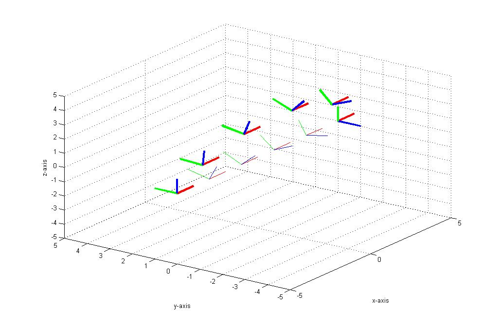
Figure 11: Comparision of Exponential map and $C^{2}$ smooth interpolation in $SE(3)$ between $g_{0}=[0,0,0]\ltimes[-5,0,0]$ and $g_{1}=[\pi/2,0,0]\ltimes[5,0,0]$, with tangents $v_{0}^{1}=[0,0,0,3,1,1]$ and $v_{2}^{1}=[\pi/2,0,0,-1,-3,-1]$.

Suppose we do not know the velocities at the node points. For such a case we have used a partial geodesic scheme to interpolate between two elements of $SE(3)$. Where, the rotational part is interpolated by the $\exp$ map and the translational component is a interpolated with spline segments.

6 Simulations

6.1 Curves on a Sphere

We begin our simulations with examples of curves on a unit sphere. We show two curves with different densities required by the MST for correct reordering of the samples.

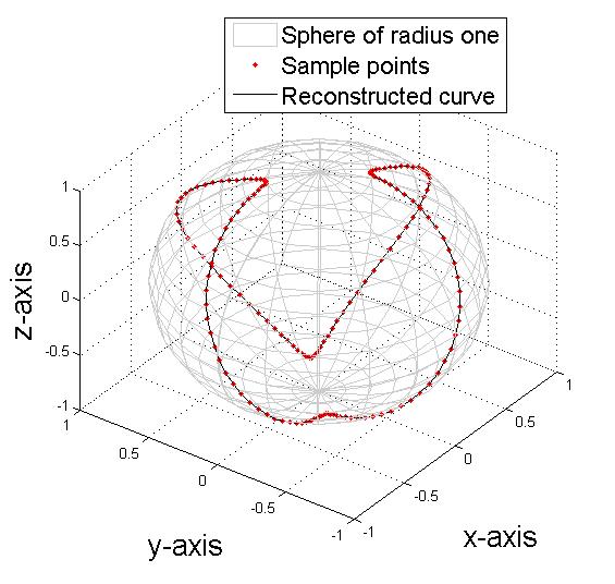
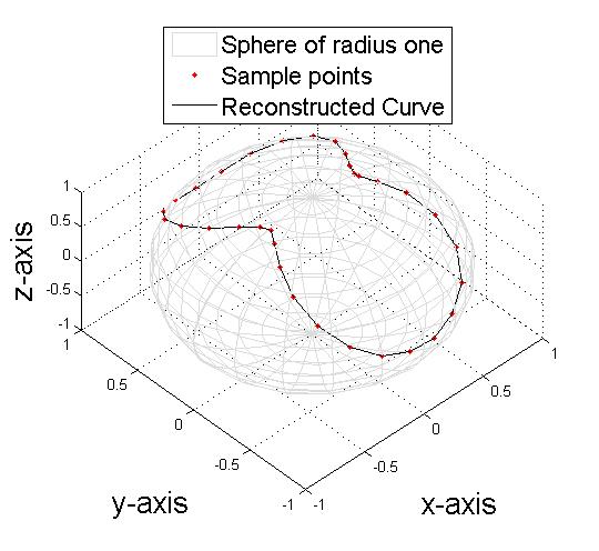
Figure 12: Example curves on a unit sphere.

The curves after reordering the sample points are shown in Fig.12 and Fig.12.

6.2 Curves in $SE(3)$

In Fig.13 an unordered set of frames in $SE(3)$ are shown. We assume that the sample shown is dense.

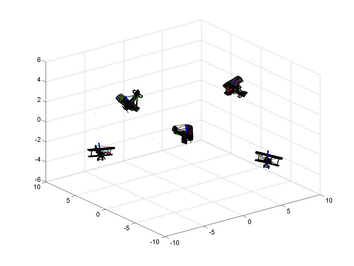
Figure 13: A sample $\mathcal{S}$ of a curve $\mathcal{C}\subset SE(3)$

By the distance metric defined in Eqn.15 we compute distances between all the frames. Finally we compute the MST for the complete weighted graph of frames with the computed distances as the edge weights.

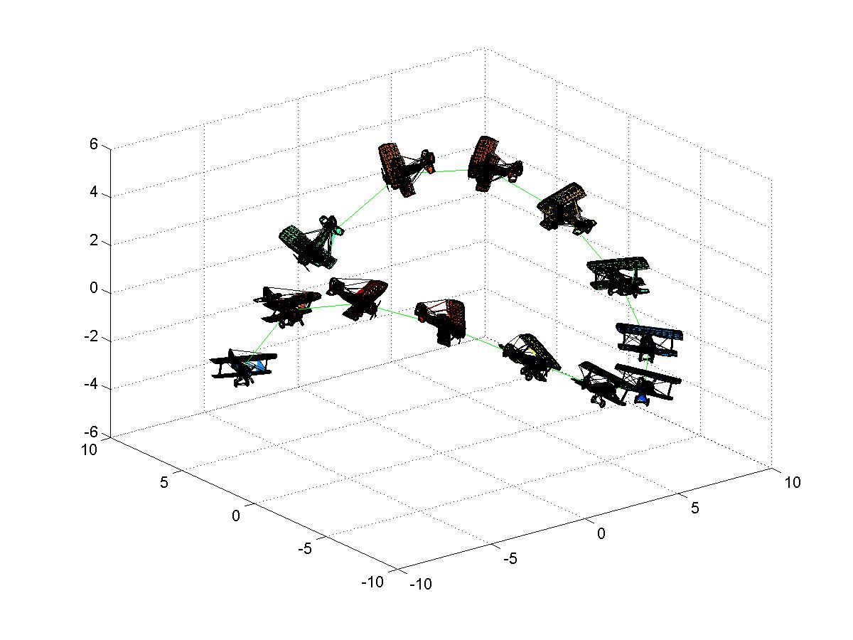
Figure 14: Reconstructed curve in $SE(3)$

Once the ordering is done we interpolate the sample with partial geodesic scheme. Results of interpolation with two different granularities is presented in Fig.14 and Fig.15.

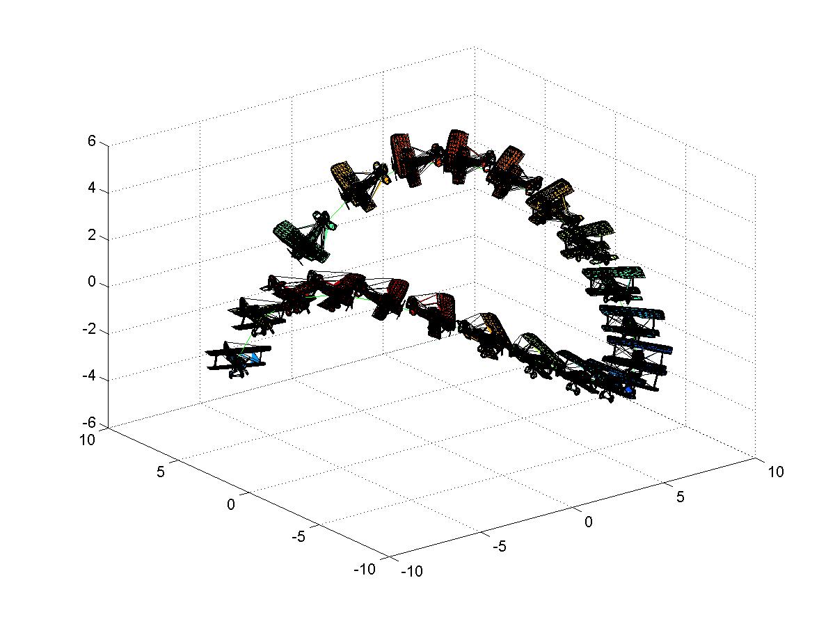
Figure 15: Reconstructed curve in $SE(3)$ with finer interpolation

6.3 Curve in $SE(3)$ with scaling parameter

Suppose for a planar object in motion, we include scaling with respect to the center of mass along with the rotation and translation. The resultant element will be of the following form

$$A=\left[\begin{array}[]{cc}e^{\lambda}R&d\\ 0&1\end{array}\right].$$ (20)

This element operates on the point of the object in plane. It scales($e^{\lambda}$) and rotates($R$) the object with respect to its center of mass and then translates($d$) the center of mass. With each such element we can associate a vector $[\lambda,\theta,d_{x},d_{y}]$. The elements of the form given by Eq.20 with standard matrix multiplication forms a lie group. We can extend the notions of tangent space and exponential map to this lie group. As discussed previously in Sec.3.2 this group is a semi-direct product of elements of scaled rotations and translations. The tangent space elements at identity, lie algebra elements, for scaled rotations are given by

$$[a]=\lambda\left[\begin{array}[]{cc}1&0\\ 0&1\end{array}\right]+\theta\left[\begin{array}[]{cc}0&-1\\ 1&0\end{array}\right]$$ (21)

And the usual matrix exponentiation gives

$$\exp{[a]}=e^{\lambda}\left[\begin{array}[]{cc}\cos{\theta}&-\sin{\theta}\\ \sin{\theta}&\cos{\theta}\end{array}\right].$$ (22)

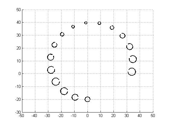
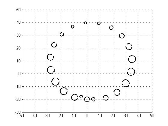
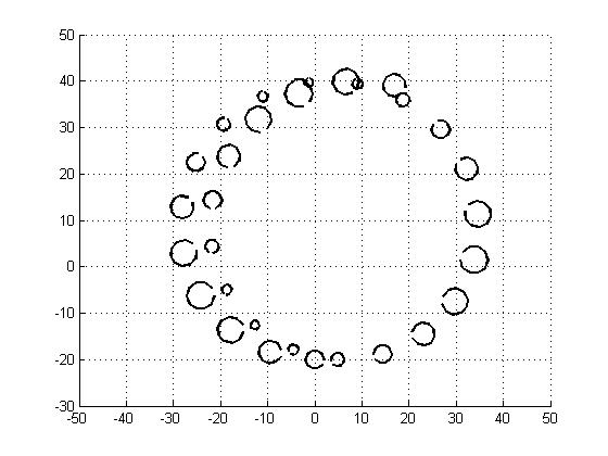
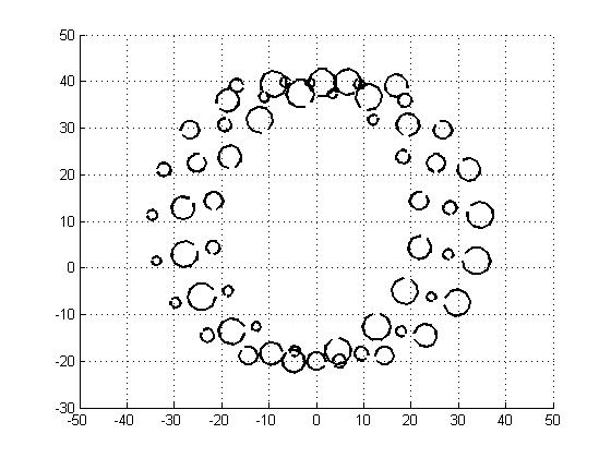
Figure 16: Various instances of a curve in $SE(2)$ with scaling.

We can construct a left-invariant riemannian metric on this group. It can be shown that for two elements $A_{1},A_{2}$ in this group

$$d(A_{1},A_{2})=\sqrt{\alpha((\lambda_{1}-\lambda_{2})^{2}+(\theta_{1}-\theta_{2})^{2})+\beta\parallel d_{1}-d_{2}\parallel}$$ (23)

is a valid distance metric. In Fig.16, a circular object under the action of this group is shown for various time steps.

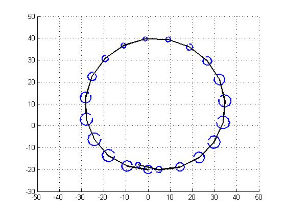
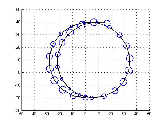
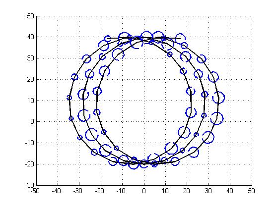
Figure 17: Instances of the reconstructed curve in $SE(3)$ with scaling.

Assuming the curve is sampled densely, along with the distance measured by Eq.23 we reconstruct the curve using MST. The successfully reconstructed curve, with the values $\alpha=10$ and $\beta=1$, is shown in Fig.17. Important fact to note here is that the curve presented here is not a closed curve. The algorithm is modified in this case to take care of the end points. In fact a simple nearest neighbour search will also do the job of reconstruction once we give in the initial point.

6.4 Application to video frame sequencing

As an application of the curve reconstruction we take up a task of ordering the frames $\{F_{i}\}_{i=1,\ldots,N}$ of a video sequence. In Fig.18 there are sixteen frames of a video sequence.

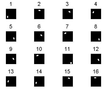
Figure 18: Unordered video frames

We use the rigid euclidean motion of an object in the frames as a clue for re-ordering the frames. Let us assume that the object under observation is masked by a rectangle and it is segmented out of the frames. We also assume that the motion of the object is the rigid body euclidean motion in $\mathbb{R}^{2}$. Further let the video frames from the sequence form a dense sample set of the motion curve. As discussed in section 3.2 we calculate the distances between frames as the distance between elements of $SE(2)$. Although we do not focus on how to estimate the rotations we give a very primitive looking argument below to estimate the distances between two frames. And it turns out that the estimates are good enough in this case to reconstruct the curve. But in general we use the $[\theta,x,y]$ as the element of $SE(2)$ and we assume that we have an oracle to give these frame coordinates to the algorithm.

The euclidean distances between the means found out from the relative positions of the rectangle is the first part of the distance metric. Next we estimate the rotation angle of the object with respect to a fixed inertial frame.

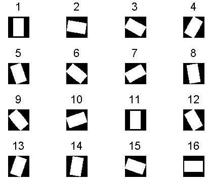
Figure 19: Mean cancellation and rotation estimation

For this purpose first we register the objects with their means. An observation reveals that if we overlap the registered rectangles the area of the overlapping region provides a good estimate of the rotation angle. In fact as shown in Fig. for $\theta>\arctan(\frac{b}{a})$, the overlapped area is $\frac{a^{2}}{\sin{\theta}}$, where $a$ is the shorter side of the rectangle. Which clearly indicates as $\theta$ increase the overlapping area decreases upto $\theta=\pi/2$. For calculating the area we count the number of lattice points(pixels) inside the overlapping regions.

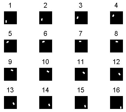
Figure 20: Ordered video frames

Finally with the estimate for $\theta$ combined with the euclidean distance between means give the $d^{*}(F_{1},F_{2})$. Using sequential search with known initial frame we re-order the frames see Fig.20. Even if we do not know about the initial frame, MST computes the correct connections of the frames and gives a correct ordering upto end points.

Let us reconsider the distance metric on $SE(2)$ given by Eqn.6. If we scale the three axis properly the problem of curve reconstruction in $SE(2)$ reduces to the problem of curve reconstruction in $\mathbb{R}^{3}$ and we may use all the non-uniform sampling schemes and voronoi diagram based reconstruction algorithms. As an example we have used NN-CRUST to reconstruct the curve above in the motion sequence and we get the correct ordering as expected.

7 Conclusion

We showed that the MST gives the correct geodesic polygonal approximation to the smooth, closed and simple curves in riemannian manifolds if the sample is dense enough and we work inside the injectivity radius. We have worked out a conservative bound on the uniform sampling of the curve. The effect of local topological behaviour of the underlying manifold was clearly identified and resolved by working inside the injectivity radius. In general the scheme works for the smooth arcs with endpoints also. We have presented simulations for successfully reconstructed curves in $SE(2)$ and $SE(3)$. We have also shown the applications of the combinatorial curve reconstruction for ordering motion frames in graphics and robotics.

If we work inside the injectivity radius of the underlying manifold we have taken care of the topological changes but to take care of geometric changes we need to work inside the convexity radius as prescribed in [13]. We believe that the results of non uniform sampling for curves in $\mathbb{R}^{n}$ are transferable to the curves in riemannian manifold with careful modifications. As an extension to this work we would like to work out the necessary proofs and carry out simulations for supporting our belief.

Appendix A Exponential and Logarithmic maps

A 1.

Given $[\omega]\in so(3)$,

$$\exp[\omega]=I+\frac{\sin\|\omega\|}{\|\omega\|}\cdot[\omega]+\frac{1-\cos\|\omega\|}{\|\omega\|^{2}}\cdot[\omega]^{2}$$ (24)

A 2.

Let $(\omega,v)\in se(3)$. Then

$$\exp\left[\begin{array}[]{cc}[\omega]&v\\ 0&0\end{array}\right]=\left[\begin{array}[]{cc}\exp[\omega]&Av\\ 0&1\end{array}\right]$$ (25)

where

$$A=I+\frac{1-\cos\|\omega\|}{\|\omega\|^{2}}\cdot[\omega]+\frac{\|\omega\|-\sin\|\omega\|}{\|\omega\|^{3}}\cdot[\omega]^{2}$$

A 3.

Given $\theta\in SO(3)$ such that $Tr(\theta)\neq-1$. Then

$$\log(\theta)=\frac{\phi}{2\sin\phi}(\theta-\theta^{T})$$ (26)

where $\phi$ satisfies $1+2\cos\phi=Tr(\theta)$, $|\phi|<\pi$. Further more, $\|\log\theta\|^{2}=\phi^{2}$.

A 4.

Suppose $\theta\in SO(3)$ such that $Tr(\theta)\neq-1$, and let $b\in\mathbb{R}^{3}$. Then

$$\log\left[\begin{array}[]{cc}\theta&b\\ 0&1\end{array}\right]=\left[\begin{array}[]{cc}[\omega]&A^{-1}b\\ 0&0\end{array}\right]$$ (27)

where $[\omega]=\log\theta$, and

$$A^{-1}=I-\frac{1}{2}\cdot[\omega]+\frac{2\sin\|\omega\|-\|\omega\|(1+\cos\|\omega\|)}{2\|\omega\|^{2}\sin\|\omega\|}\cdot[\omega]^{2}$$

A 5.

Let $\theta_{1},\theta_{2}\in SO(3)$. Then the distance $L=d(\theta_{1},\theta_{2})$ induced by the standard bi-invariant metric on $SO(3)$ is

$$d(\theta_{1},\theta_{2})=\|\log(\theta_{1}^{-1}\theta_{2})\|$$ (28)

where $\|\cdot\|$ denotes the standard Euclidean norm.

A 6.

Let $X_{1}=(\theta_{1},b_{1})$ and $X_{2}=(\theta_{2},b_{2})$ be two points in $SE(3)$. Then the distance $L=d(X_{1},X_{2})$ induced by the scale dependent left-invariant metric on $SE(3)$ is

$$d(X_{1},X_{2})=\sqrt{c\|\log(\theta_{1}^{-1}\theta_{2})\|^{2}+d\|b_{2}-b_{1}\|^{2}}$$ (29)

where $\|\cdot\|$ denotes the Euclidean norm.

References

- [1] L. H. de Figueiredo and J. de Miranda Gomes, “Computational morphology of curves,” The Visual Computer, no. 11, pp. 105–112, 1994.
- [2] N. Amenta, M. Bern, and D. Eppstein, “The crust and the -skeleton: Combinatorial curve reconstruction.” Graph. Models Image Process., no. 60, pp. 125–135, 1998.
- [3] H. Edelsbrunner, “Shape reconstruction with delaunay complex,” LATIN’98 LNCS 1380: Theoretical Informatics, pp. 119–132, 1998.
- [4] T. K. Dey, Curve and Surface Reconstruction: Algorithms with Mathematical Analysis, P. G. Ciarlet, A. Iserles, R. V. Kohn, and M. H. Wright, Eds. Cambridge, 2007.
- [5] E. Althaus et al., “Experiments on curve reconstruction.”
- [6] T. K. Dey and P. Kumar, “A simple provable curve reconstruction algorithm,” pp. 893–894, 1999.
- [7] A. Gray, E. Abbena, and S. Salamon, Modern Differential Geometry of Curves and Surfaces with Mathematica, ser. Studies in advanced mathematics. Chapman & Hall/CRC, 2006.
- [8] R. Kimmel and J. A. Sethian, “Computing geodesic paths on manifolds,” in Proc. of National Academy of Sciences, USA, vol. 95, no. 15, 1998, pp. 8431–8435.
- [9] J. M. Selig, Geometric Fundamentals of Robotics, ser. Monographs in Computer Science. Springer, 2005.
- [10] M. Zefran, V. Kumar, and C. Croke, “On the generation of smooth three-dimensional rigid body motions,” IEEE Transactions on Robotics and Automation, 1995.
- [11] F. C. Park, “Distance metrics on the rigid-body motions with applications to mechanism design,” ASME Journal of Mechanism Design, vol. 117, no. 1, pp. 48–54, 1995.
- [12] J. O’Rourke, Computational Geometry in C, 2nd ed. Cambridge University Press, 1998.
- [13] G. Leibon and D. Letscher, “Delaunay triangulations and voronoi diagrams for riemannian manifolds,” in Symposium on Computational Geometry, 2000, pp. 341–349.
- [14] M. Spivak, Differential Geometry. Publish or Perish, Inc., 2005, vol. 1.
- [15] M. P. do Carmo, Riemannian Geometry. Birkhauser, 1992.
- [16] K. Shoemake, “Animating rotation with quaternion curves,” SIGGRAPH Comput. Graph., vol. 19, no. 3, pp. 245–254, 1985.
- [17] M.-J. Kim, M.-S. Kim, and S. Y. Shin, “A -continuous b-spline quaternion curve interpolating a given sequence of solid orientations,” Computer Animation, vol. 0, p. 72, 1995.
- [18] F. C. Park and B. Ravani, “Smooth invariant interpolation of rotations,” ACM Transactions on Graphics, vol. 16, no. 3, pp. 277–295, July 1997.
- [19] J. Li and P.-w. Hao, “Smooth interpolation on homogeneous matrix groups for computer animation,” Journal of Zhejiang University - Science A, vol. 7, pp. 1168–1177, 2006, 10.1631/jzus.2006.A1168. [Online]. Available: http://dx.doi.org/10.1631/jzus.2006.A1168
- [20] C. Altafini, “The de casteljau algorithm on se(3),” in Nonlinear control in the Year 2000, ser. Lecture Notes in Control and Information Sciences, A. Isidori, F. Lamnabhi-Lagarrigue, and W. Respondek, Eds. Springer Berlin / Heidelberg, 2000, vol. 258, pp. 23–34, 10.1007/BFb0110205. [Online]. Available: http://dx.doi.org/10.1007/BFb0110205