Static interactions and stability of matter in Rindler space

Abstract

Dynamical issues associated with quantum fields in Rindler space are addressed in a study of the interaction between two sources at rest generated by the exchange of scalar particles, photons and gravitons. These static interaction energies in Rindler space are shown to be scale invariant, complex quantities. The imaginary part will be seen to have its quantum mechanical origin in the presence of an infinity of zero modes in uniformly accelerated frames which in turn are related to the radiation observed in inertial frames. The impact of a uniform acceleration on the stability of matter and the properties of particles is discussed and estimates are presented of the instability of hydrogen atoms when approaching the horizon.

I Introduction

The study of quantum fields in Rindler space has played an important role in developing our understanding of quantum fields in non-trivial space-times. The importance of these studies derives to a large extent from the existence of a horizon in Rindler space. With its close connection to Minkowski space via the known local relation between fields in uniformly accelerated and inertial frames, Rindler space provides the simplest possible context to investigate kinematics and dynamics of quantum fields close to a horizon.

The kinematics of non-interacting quantum fields in Rindler space FULL73 , BOUL75 , DAVI75 and their relation to fields in Minkowski space together with the interpretation in terms of quantum fields at finite temperature UNRU76 , SCCD81 are well understood. The relation between acceleration and finite temperature remains an important element of the thermodynamics of black holes. Although formally established, the relation between fields in Rindler and Minkowski spaces has posed some intriguing interpretational problems. Here we mention in particular the issue of compatibility of the radiation generated by a uniformly accelerated charge observed in Minkowski space and the apparent absence of radiation in the coaccelerated frame. This problem was finally resolved by the realization that the counterpart of Minkowski space radiation is the emission of zero energy photons in Rindler space HIMS921 , HIMS922 , REWE94 . Dynamical issues of quantum fields have received less attention (cf. CRHM07 ). Related to topics to be discussed in the following are the study of the relation between interacting quantum fields in Minkowski and Rindler spaces within the path-integral formalism UNRU84 , the calculation of level shifts in accelerated hydrogen atoms PASS98 and the investigations of the decay of protons MULL97 , VAMA00 .

Dynamical issues of quantum fields in Rindler space are in the center of our work. Subject are static forces and their properties relevant for the structure of matter in Rindler space. We will study the forces acting between static scalar sources, electric charges and massive sources generated by exchange of massless scalar particles, photons and gravitons respectively. The relevant quantities involved are the corresponding static Rindler space propagators. While the time dependent propagators in Rindler and Minkowski spaces are trivially related to each other by a coordinate transformation with corresponding mixing of the components, this is not the case for the static propagators obtained by integration over the corresponding time. The different properties of the static propagators reflect the significant differences of Rindler and Minkowski space Hamiltonians. Though it was realized from the beginning that the interpretation of Rindler and Minkowski particles (cf. e.g. FULL73 ) is different, the differences in the corresponding Hamiltonians have not received sufficient attention. (The identity of the Rindler and Minkowski space Hamiltonians for the frequently used special case of a massless field in two dimensional space-time may have obscured the issue.) As shown in LOY08 , the Rindler space Hamiltonian exhibits symmetries which give rise to a highly degenerate spectrum. In particular this degeneracy is also present in the zero energy sector. This 2-dimensional sector of zero modes is the image of the photons generated by the charges uniformly accelerated in Minkowski space. It will be shown to give rise to an unexpected quantum mechanical contribution to the force acting between two charges. Also the classical Coulomb-like contribution to the force will be shown to significantly deviate from the electrostatic force in Minkowski space. The electrostatic force will be determined via Wilson loops and Polyakov loop correlation functions. This method will enable us to separate the contribution of the quantum mechanical transverse photons from that of the classical longitudinal field. It will be the method of choice if one attempts to determine the static force in simulations of non-abelian gauge theories on a Rindler space lattice.

The modifications in the interaction of two charges at rest in Rindler space raise naturally the question of the stability of atomic systems in Rindler space. We shall investigate this issue for an ensemble of hydrogen atoms and show within a non-relativistic reduction that indeed only metastable states exist. We will estimate the probability of ionization as a function of the distance to the horizon and present arguments concerning the stability of other forms of matter.

II Propagators and interactions of scalar particles in Rindler space

II.1 The quantized scalar field in Rindler space

The Rindler space metric RIND01

$$ds^{2}=e^{2a\xi}(d\tau^{2}-d\xi^{2})-d{\bf x}^{2}_{\perp}\,,$$ (1)

is the (Minkowski) metric seen by a uniformly accelerated observer (acceleration $a$ in $x^{1}$-direction). Rindler space ($\tau,\xi$) and Minkowski space ($t,x^{1}$) coordinates are related by

$$t(\tau,\xi)=\frac{1}{a}\;e^{a\xi}\sinh a\tau\,,\quad x^{1}(\tau,\xi)=\frac{1}{a}\;e^{a\xi}\cosh a\tau\,.$$ (2)

The range of $\tau,\,\xi$ is

$$-\infty\;\leq\;\tau\,,\xi\;\leq\;\infty\,,$$ (3)

while the preimage of the Rindler space covers only part of Minkowski space, the right “Rindler wedge”,

$$R_{+}=\big{\{}x^{\mu}\big{|}\,|t|\leq x^{1}\big{\}}\,.$$ (4)

The restriction of the preimage of the Rindler space to the right Rindler wedge gives rise to a horizon, the boundary $t=\pm x^{1},\,\,\text{i.e.}\,\,\xi=-\infty$. With this property the Rindler metric can be identified with other static metrics in the near horizon limit. In particular this is the case for the Schwarzschild metric which can be approximated in the limit that the distance from the horizon is small in comparison to the Schwarzschild radius and if the spherical Schwarzschild horizon is replaced by a tangential plane.

We start our study of propagators and interactions with a discussion of a scalar field in Rindler space (cf. for instance FULL73 , CRHM07 . We will use the notation of LOY08 ). The action of a free massive scalar field is given by

$$S=\frac{1}{2}\int d\tau\;d\xi\;d^{\,2}x_{\perp}\big{\{}\partial_{\tau}\phi)^{2}-(\partial_{\xi}\phi)^{2}-(m^{2}\phi^{2}+(\boldsymbol{\partial}_{\perp}\phi)^{2})\;e^{2a\xi}\big{\}}\,.$$ (5)

The wave equation

$$\Big{[}\partial^{2}_{\tau}-\Delta_{s}+m^{2}e^{2a\xi}\Big{]}\phi=0\,,$$ (6)

with the Laplacian

$$\Delta_{s}=\partial^{2}_{\xi}+e^{2a\xi}\partial_{\perp}^{2}\,,$$ (7)

is solved by the normal modes (in terms of the McDonald functions)

$$\phi_{\omega,{\bf k}_{\perp}}(\xi,{\bf x_{\perp}})=\frac{1}{\pi}\;\sqrt{2\frac{\omega}{a}\sinh\pi\frac{\omega}{a}}\;K_{i\frac{\omega}{a}}\Big{(}\frac{1}{a}\sqrt{m^{2}+{\bf k}^{2}_{\perp}}e^{a\xi}\Big{)}\,e^{i{\bf k}_{\perp}{\bf x}_{\perp}}\,,$$ (8)

which form a complete, orthonormal set of functions. The normal mode expansion of the scalar field $\phi$ reads

$$\phi(\tau,\xi,{\bf x}_{\perp})=\int\frac{d\omega}{\sqrt{2\omega}}\frac{d^{2}k_{\perp}}{2\pi}\Big{(}a(\omega,{\bf k}_{\perp})\phi_{\omega,{\bf k}_{\perp}}(\xi,{\bf x_{\perp}})e^{-i\omega\tau}+a^{\dagger}(\omega,{\bf k}_{\perp})\phi^{\star}_{\omega,{\bf k}_{\perp}}(\xi,{\bf x_{\perp}})e^{i\omega\tau}\Big{)}$$ (9)

with the creation and annihilation operators $a^{(\dagger)}$. The stationary states associated with the Hamiltonian ($\pi=\partial_{\tau}\phi)\,$

$$H_{R} = \frac{1}{2}\int d\xi d^{2}x_{\perp}\big{\{}\pi^{2}+(\partial_{\xi}\phi)^{2}+\,e^{2a\xi}\big{(}m^{2}\phi^{2}+(\boldsymbol{\partial}_{\perp}\phi)^{2}\big{)}\big{\}}$$ (10)

$$= \int d^{2}k_{\perp}\int^{\infty}_{0}d\omega\,\omega a^{\dagger}(\omega,{\bf k}_{\perp})a(\omega,{\bf k}_{\perp})\,,$$

including the lowest energy ($\omega=0$) state, are degenerate with respect to the value of the transverse momentum ${\bf k}_{\perp}$. This degeneracy has its origin in the appearance of the transverse momentum (in combination with the mass) as a coupling constant of the “inertial potential” $e^{2a\xi}$ in the Hamiltonian.

In the Rindler wedge (4), the field operator $\phi$ can be represented in terms of plane waves in Minkowski space or in terms the Rindler space normal modes (9) resulting in the representation of the Rindler creation and annihilation operators in terms of the corresponding Minkowski space operators. This relation yields the important result for the expectation value of the Rindler number operator in the Minkowski ground state $|0_{M}\rangle$

$$\langle 0_{M}|a^{\dagger}(\omega,{\bf k}_{\perp})a(\omega^{\prime},{\bf k}_{\perp}^{\prime})|0_{M}\rangle=\frac{1}{e^{2\pi\frac{\omega}{a}}-1}\delta(\omega-\omega^{\prime})\delta({\bf k}_{\perp}-{\bf k}^{\prime}_{\perp})\,$$ (11)

which exhibits a thermal distribution with temperature

$$T=\frac{1}{\beta}=\frac{a}{2\pi}\,.$$ (12)

It is important to realize that the infinite degeneracy of the Rindler eigenstates leads, at long wavelengths, effectively to 1-dimensional thermal distributions with weight $d\omega/(e^{2\pi\frac{\omega}{a}}-1)$ .

II.2 The scalar Rindler space propagator

The propagators in Minkowski and Rindler spaces are related to each other by the coordinate transformation (2). Written in terms of Rindler and Minkowski coordinates respectively, the propagator of a massless field is given by (cf. TRDA77 , DOWK78 )

$$D(\tau-\tau^{\prime},\xi,\xi^{\prime},{\bf x}_{\perp}-{\bf x}_{\perp}^{\prime})=i\langle 0_{M}\big{|}T\big{[}\phi(\tau,\xi,{\bf x}_{\perp})\phi(\tau^{\prime},\xi^{\prime},{\bf x}_{\perp}^{\prime})\big{]}\big{|}0_{M}\rangle=D(x-x^{\prime})$$

$$=\frac{1}{4i\pi^{2}\big{(}(x-x^{\prime})^{2}-i\delta\big{)}}=\frac{a^{2}e^{-a(\xi+\xi^{\prime})}}{8i\pi^{2}}\frac{1}{\cosh a(\tau-\tau^{\prime})-\cosh\eta-i\delta}\,,$$ (13)

with the notations

$$D(\tau-\tau^{\prime},\xi,\xi^{\prime},{\bf x}_{\perp}-{\bf x}_{\perp}^{\prime})=D(x(\tau,\xi,{\bf x}_{\perp})-x(\tau^{\prime},\xi^{\prime},{\bf x^{\prime}}_{\perp}))$$ (14)

and

$$\cosh\eta(\xi,\xi^{\prime},{\bf x}_{\perp}-{\bf x}_{\perp}^{\prime})=1+\frac{\big{(}e^{a\xi}-e^{a\xi^{\prime}}\big{)}^{2}+a^{2}\big{(}{\bf x}_{\perp}-{\bf x}_{\perp}^{\prime}\big{)}^{2}}{2e^{a(\xi+\xi^{\prime})}}=1+\sigma^{2}(\xi,\xi^{\prime},{\bf x}_{\perp}-{\bf x}_{\perp}^{\prime})\,.$$ (15)

As we will see, it is $\eta$ (or equivalently $\sigma$) which determines the interaction energies rather than the proper distance in Rindler space

$$d(\xi,\xi^{\prime},{\bf x}_{\perp}-{\bf x}_{\perp}^{\prime})=\sqrt{\frac{1}{a^{2}}\big{(}e^{a\xi}-e^{a\xi^{\prime}}\big{)}^{2}+\big{(}{\bf x}_{\perp}-{\bf x}_{\perp}^{\prime}\big{)}^{2}}\,.$$ (16)

The quantity $\eta$ actually can be viewed as the proper distance in the 4-dimensional AdS space. The appearance of this geometry (of a three-hyperboloid) has been noted SCCD81 in the context of the unusual density of states in the photon energy momentum tensor in Rindler space. The quantity $\eta$ or equivalently $\sigma$ exhibits the remarkable invariance under the transformation

$$\xi,\,\xi^{\prime}\to\xi+\xi_{0},\,\xi^{\prime}+\xi_{0}\,,\quad{\bf x}_{\perp},\,{\bf x}_{\perp}^{\prime}\to e^{a\xi_{0}}{\bf x}_{\perp},\,e^{a\xi_{0}}{\bf x}_{\perp}^{\prime}\,.$$ (17)

The coordinate transformation (17) together with a rescaling of the fields $\phi(\tau,\xi,{\bf x}_{\perp})\to e^{a\xi_{0}}\phi(\tau,\xi,{\bf x}_{\perp})$ leaves, for $m=0$, the Hamiltonian (10) invariant and gives rise to the degeneracy of the spectrum. The invariance under scale transformations can be generalized to massive particles LOY08 .

In Rindler space coordinates the 2-point function (13) satisfies

$$\big{(}\partial_{\tau}^{2}-\partial_{\xi}^{2}-e^{2a\xi}\partial_{\perp}^{2}\big{)}D(\tau,\xi,\xi^{\prime},{\bf x}_{\perp})=\delta(\tau)\delta(\xi-\xi^{\prime})\delta({\bf x}_{\perp})\,.$$ (18)

After a Wick rotation of the Rindler time,

$$\tau\to\tau_{E}=-i\tau\,,$$ (19)

the propagator is periodic in the imaginary time with periodicity $\beta$ (cf. Eq. (12))

$$D_{\text{E}}(\tau_{\text{E}},\xi,\xi^{\prime},{\bf x}_{\perp})=\frac{a^{2}e^{-a(\xi+\xi^{\prime})}}{8i\pi^{2}}\frac{1}{\cos a\tau_{\text{E}}-\cosh\eta-i\delta}\,.$$ (20)

In the context of the electromagnetic field we will compute observables in both the real and imaginary Rindler time formalisms. (For discussions of “Euclidean” Rindler space propagators, in particular of their topological interpretation cf. CHDU78 , LINE95 , SVZA08 .)

Without reference to the Minkowski space propagator, Eq. (13) can be derived alternatively via the normal mode decomposition (9) in Rindler space. With the help of Eq. (11) the result

$$D(\tau,\xi,\xi^{\prime},{\bf x}_{\perp})=D^{(R)}(\tau,\xi,\xi^{\prime},{\bf x}_{\perp})+i\int_{0}^{\infty}\frac{d\Omega}{\Omega}\int\frac{d^{2}k_{\perp}}{(2\pi)^{2}}\phi_{\Omega,{\bf k}_{\perp}}(\xi,{\bf x_{\perp}})\phi_{\Omega,{\bf k}_{\perp}}(\xi^{\prime},{\bf 0_{\perp}})\frac{\cos{\Omega\tau}}{e^{\frac{2\pi\Omega}{a}}-1}$$

(21)

is obtained where the propagator defined with respect to the Rindler space vacuum is given by

$$D^{(R)}(\tau,\xi,\xi^{\prime},{\bf x}_{\perp})=i\langle 0_{R}\big{|}T\big{[}\phi(\tau,\xi,{\bf x}_{\perp})\phi(0,\xi^{\prime},{\bf 0}_{\perp})\big{]}\big{|}0_{R}\rangle$$

$$=i\int_{0}^{\infty}\frac{d\Omega}{2\Omega}\int\frac{d^{2}k_{\perp}}{(2\pi)^{2}}\phi_{\Omega,{\bf k}_{\perp}}(\xi,{\bf x_{\perp}})\phi_{\Omega,{\bf k}_{\perp}}(\xi^{\prime},{\bf 0_{\perp}})e^{-i\Omega|\tau|}=\frac{a^{2}e^{-a(\xi+\xi^{\prime})}\eta}{4i\pi^{2}\,\sinh\eta}\frac{1}{a^{2}\tau^{2}-\eta^{2}-i\delta}\,.$$ (22)

(For an interpretation of the difference between the two propagators $D-D^{(R)}$ in terms of image charges located in the left Rindler wedge $|t|\leq-x^{1}$, cf. CARA76 .) Obviously, the propagator $D^{(R)}$ depends parametrically on the acceleration $a$. In order to formulate properly the relation between propagators in Minkowski and Rindler spaces one has to define the Rindler space propagator for a fixed value of the acceleration $a$ at finite temperature (given by $\beta$)

$$D_{a,\beta}(\tau,\xi,\xi^{\prime},{\bf x}_{\perp})=i\frac{1}{\text{tr}\,e^{-\beta H_{R}(a)}}\text{tr}\,\Big{\{}e^{-\beta H_{R}(a)}T\big{[}\phi(\tau,\xi,{\bf x}_{\perp})\phi(0,\xi^{\prime},{\bf 0}_{\perp})\big{]}\Big{\}}\,.$$ (23)

In terms of the propagator $D_{a,\beta}$, the central result concerning the relation between Rindler and Minkowski spaces is the identity

$$i\langle 0_{M}\big{|}T\big{[}\phi(\tau,\xi,{\bf x}_{\perp})\phi(0,\xi^{\prime},{\bf 0}_{\perp})\big{]}\big{|}0_{M}\rangle=D_{a,\frac{2\pi}{a}}(\tau,\xi,\xi^{\prime},{\bf x}_{\perp})\,,$$ (24)

i.e., the Rindler space propagator defined with respect to the Minkowski ground state coincides with the Rindler space finite temperature propagator with the value of the temperature determined by the acceleration $a$ (cf. Eq. (12)). This identity makes also manifest that a change in the acceleration $a$ does not correspond to a change in temperature of the accelerated system. The acceleration appears not only as temperature in the Boltzmann factor but also as a parameter in the Hamiltonian (10) of the accelerated system. We will encounter observables which make explicit this twofold role of the acceleration.

The basic quantity in the following investigation of the properties and consequences of interactions generated by exchange of scalar particles and photons is the static propagator

$$\tilde{D}(\omega,\xi,\xi^{\prime},{\bf x}_{\perp})=\int_{-\infty}^{\infty}d\tau e^{i\omega\tau}D(\tau,\xi,\xi^{\prime},{\bf x}_{\perp})\,.$$ (25)

For vanishing mass the $k_{\perp}$-integration in (21) can be carried out in closed form (cf. RG65 and EMOT53 )

$$\tilde{D}(\omega,\xi,\xi^{\prime},{\bf x}_{\perp})=\frac{a}{4\pi e^{a(\xi+\xi^{\prime})}\sinh{\eta}}\Big{(}e^{i\frac{|\omega|\eta}{a}}+\frac{2i\sin{\frac{|\omega|\eta}{a}}}{e^{\frac{2\pi|\omega|}{a}}-1}\Big{)}\,.$$ (26)

Alternatively, this result can be obtained by a contour integration of Eq. (13) in the complex $\tau$ plane. The first term is due to the pole infinitesimally close to the real axis $\tau=\eta+i\delta$ while the second, imaginary contribution is the result of the summation of the residues of the poles at $\tau_{n}=\eta+2in\pi,\;n\geq 1$. The result for the static propagator and its decomposition into the real non-thermal and the imaginary thermal contributions read

$$\tilde{D}(0,\xi,\xi^{\prime},{\bf x}_{\perp})=\tilde{D}^{(R)}(0,\xi,\xi^{\prime},{\bf x}_{\perp})+\frac{i}{2\pi\beta}\frac{\eta}{e^{a(\xi+\xi^{\prime})}\,\sinh\eta}\big{|}_{\beta=\frac{2\pi}{a}}=\frac{a}{4\pi e^{a(\xi+\xi^{\prime})}}\frac{1}{\sinh\eta}\Big{[}1+\frac{i\eta}{\pi}\Big{]}\,.$$ (27)

The imaginary part of the static propagator $\tilde{D}$ arises since the propagator (21) is defined with respect to the Minkowski rather than to the Rindler ground state.

II.3 The interaction energy of scalar sources

Given the propagator, the interaction energy between two scalar sources is obtained by adding to the action (5) the scalar particle-source vertex

$$S_{\text{int}}=-\int dv^{0}H_{\text{int}}=\kappa_{0}\int d^{4}v\sqrt{|g(v)|}\,\rho(v)\,\phi(v)\,\,,$$ (28)

where $v$ stands for either Minkowski ($x$) or Rindler coordinates ($\tau,\xi,{\bf x}_{\perp}$). The effective action (the generating functional of connected diagrams) associated with the source is given by

$$W_{\text{sc}}=-\frac{1}{2}\kappa_{0}^{2}\int d^{4}v\sqrt{|g(v)|}\,\rho(v)\,\int d^{4}v^{\prime}\sqrt{|g(v^{\prime})|}\,\rho(v^{\prime})\,D(v,v^{\prime})\,.$$ (29)

For two point like sources moving along the trajectories $v_{i}(s_{i})$ which are parametrized in terms of their proper times $s_{i}$, we find

$$\sqrt{|g(v)|}\rho(v)=\sum_{i=1,2}\int ds_{i}\,\delta^{4}(v-v_{i}(s_{i}))\,.$$ (30)

We assume the sources to be at rest in Rindler space and evaluate $W_{\text{sc}}$ by expressing the proper times $s_{i}$ by the coordinate times $\tau_{i}$ and obtain for sources positioned at $\xi_{i},{\bf x}_{\perp\,i}$

$$W_{\text{sc}}=-\frac{1}{2}\sum_{i,j=1,2}\kappa(\xi_{i})\kappa(\xi_{j})\int d\tau_{i}\int d\tau^{\prime}_{j}D\big{(}\tau_{i}-\tau_{j}^{\prime},\xi_{i},\xi_{j},{\bf x}_{i\,\perp}-{\bf x}_{j\,\perp}\big{)}\,.$$ (31)

We have introduced the effective coupling constant

$$\kappa(\xi)=e^{a\xi}\kappa_{0}\,,$$ (32)

which, due to the difference between proper and coordinate times,“runs” with the coordinates $\xi_{i}$ of the charges. With the sources at rest, $W_{\text{sc}}$ depends only on the differences of the times $\tau_{i}$. After carrying out the $\tau_{i}$ integrations, up to a factor $T$, the size of the interval in the integration over the sum of the times, $W_{\text{sc}}$ is determined by the static propagator and yields for $i\neq j$ the interaction energy of two scalar sources

$$V_{\text{sc}} = -\kappa(\xi_{1})\kappa(\xi_{2})\tilde{D}\big{(}\xi_{1},\xi_{2},{\bf x}_{\perp\,1}-{\bf x}_{\perp\,2}\big{)}=-\frac{a\kappa_{0}^{2}}{4\pi\sinh\eta}\Big{[}1+\frac{i\eta}{\pi}\Big{]},$$ (33)

where $\eta=\eta(\xi_{1},\xi_{2},{\bf x}_{1\,\perp}-{\bf x}_{2\,\perp})$ (cf. Eq. (15)). For two sources at rest in Minkowski space, this procedure yields the interaction energy $-\kappa_{0}^{2}/\big{|}{\bf x_{1}}-{\bf x}_{2}\big{|}$.

The interaction energy (33) constitutes an explicit example of the bivalent role of the acceleration $a$. The $a$ dependence of the real part of the interaction is exclusively due to the dependence of the Hamiltonian (10) on the parameter $a$ while the imaginary part depends in addition on the acceleration via the temperature $\beta=2\pi/a$ (cf. Eq. (27)). The appearance of a non-trivial imaginary contribution to the “static interaction” generated by exchange of scalar particles and, as we will see also by photons or gravitons, is a novel phenomenon not encountered in the static interactions in Minkowski space. Here we will analyze this phenomenon. Other properties of the interaction (33) will be discussed later in the comparison with the “electrostatic” interaction.

As follows from Eq. (18) the static propagator (27) satisfies the Poisson equation for a point-like source in Rindler space. Since the source is real, the imaginary part of the propagator satisfies the corresponding (homogeneous) Laplace equation. In turn, this implies that the imaginary part of propagator or the interaction energy can be represented by a linear superposition of zero modes of the Laplace operator (7). From Eq. (21) we read off

$$\text{Im}\,\tilde{D}(0,\xi,\xi^{\prime},{\bf x}_{\perp}-{\bf x}_{\perp}^{\prime}) = \frac{a\,\eta}{4\pi^{2}e^{a(\xi+\xi^{\prime})}\sinh\eta}$$ (34)

$$= \frac{1}{4\pi^{3}a}\int d^{2}k_{\perp}e^{i{\bf k}_{\perp}({\bf x}_{\perp}-{\bf x}^{\prime}_{\perp})}K_{0}\Big{(}\frac{k_{\perp}}{a}\,e^{a\xi}\Big{)}\,K_{0}\Big{(}\frac{k_{\perp}}{a}\,e^{a\xi^{\prime}}\Big{)}\,.$$

It is instructive to compare the Rindler space propagator with the finite temperature propagator in Minkowski space. As above we decompose the propagator of a non interacting scalar field into thermal and non-thermal contributions

$$D_{\beta}(x) = i\frac{1}{\text{tr}\,e^{-\beta H_{M}}}\text{tr}\,\Big{\{}e^{-\beta H_{M}}T\big{[}\phi(x)\phi(x^{\prime})\big{]}\Big{\}}$$ (35)

$$= \frac{im}{4\pi^{2}\sqrt{-x^{2}+i\epsilon}}K_{1}\big{(}m\sqrt{-x^{2}+i\epsilon}\,\big{)}+\delta D_{\beta}(x)\,,$$

carry out the Fourier transform of the thermal part

$$\delta\tilde{D}_{\beta}(\omega,{\bf x})=\int_{-\infty}^{\infty}dt\,\delta D_{\beta}(x)e^{i\omega t}=\frac{i}{2\pi x}\theta(\omega^{2}-m^{2})\,\frac{\sin\big{(}\sqrt{\omega^{2}-m^{2}}x\big{)}}{e^{\beta|\omega|}-1}\,,$$ (36)

and obtain for massless particles

$$m=0\,,\quad\tilde{D}_{\beta}(0,{\bf x}-{\bf x}^{\prime})=\int_{-\infty}^{\infty}dt\,D_{\beta}(t,{\bf x}-{\bf x}^{\prime})=\frac{1}{4\pi|{\bf x}-{\bf x}^{\prime}|}+\frac{i}{2\pi\beta}\,.$$ (37)

The Fourier transformed thermal propagators in Rindler (27) and in Minkowski space (37) become identical to order $O(a)$ apart from the factor $e^{-a(\xi+\xi^{\prime})}$ and differ from the corresponding ground state contribution only by the constant $i/2\pi\beta$. The convergence to this limit is not uniform in Rindler space, since it requires $a|\xi|\,,a|\xi^{\prime}|\ll 1$. Due to the twofold role of the acceleration $a$ the finite temperature contribution to the propagator in Minkowski space is only part of the leading order correction to the propagator (cf. Eq. (27)) in Rindler space. The structure of the Minkowski space static propagator suggests that the imaginary part is due to on-shell propagation of zero-energy massless particles. The difference between Rindler and Minkowski space propagators is due to the different dimensions (0 and 2 respectively) of the space of zero modes. Furthermore, while the Minkowski space zero mode is constant, the zero modes in Rindler space exhibit a non-trivial dependence on all the three coordinates. Finally for massive particles no zero mode exists in Minkowski space (Eq. (36)) while in Rindler space together with the degeneracy in the spectrum also the zero modes persist. In this case the spectral representation in Eq. (34) remains valid provided we replace $k_{\perp}^{2}\to k_{\perp}^{2}+m^{2}$ in the arguments of the McDonald functions.

The imaginary part of the propagator determines the particle creation and annihilation rates. To leading order in the coupling constant $\kappa_{0}$, the probability for a change in the initial state in the time interval $[\tau_{0},\tau]$ is given by (cf. Eqs. ((28)-(32))

$$P_{ex}(\tau,\tau_{0})=1-\Big{|}\langle 0_{M}|T\,e^{-i\int_{\tau_{0}}^{\tau}d\tau^{\prime}H_{\text{int}}(\tau^{\prime})}|0_{M}\rangle\Big{|}^{2}\approx\text{Re}\int_{\tau_{0}}^{\tau}d\tau^{\prime}\int_{\tau_{0}}^{\tau}d\tau^{\prime\prime}\langle 0_{M}\big{|}T\big{[}H_{\text{int}}(\tau^{\prime})H_{\text{int}}(\tau^{\prime\prime})\big{]}\big{|}0_{M}\rangle$$

$$\approx\text{Im}\int_{\tau_{0}}^{\tau}d\tau^{\prime}\int_{\tau_{0}}^{\tau}d\tau^{\prime\prime}\sum_{i,j=1,2}\kappa(\xi_{i})\kappa(\xi_{j})D(\tau^{\prime}-\tau^{\prime\prime},\xi_{i},\,\xi_{j},{\bf x}_{\perp\,i}-{\bf x}_{\perp\,j})\,.$$ (38)

The rate for a change in the initial state within an arbitrarily large time interval $T$ is easily obtained to be

$$\frac{1}{T}P_{ex}(T,0) \to \text{Im}\sum_{i,j=1,2}\kappa(\xi_{i})\kappa(\xi_{j})\tilde{D}(0,\xi_{i},\,\xi_{j},{\bf x}_{\perp\,i}-{\bf x}_{\perp\,j})$$ (39)

$$= \frac{\kappa_{0}^{2}a}{2\pi^{2}}\Big{(}1+\frac{\eta(\xi_{1},\xi_{2},{\bf x}_{\perp\,1}-{\bf x}_{\perp\,2})}{\sinh\eta(\xi_{1},\xi_{2},{\bf x}_{\perp\,1}-{\bf x}_{\perp\,2})}\Big{)}\,.$$

The total response (not observable in the accelerated frame) of the field to external sources determines the imaginary part of the static propagator. Furthermore by defining the reaction rate in terms of the proper time of the external sources (cf. HIMS921 , HIMS922 , CRHM07 , REWE94 ) it is seen that the imaginary part is determined by the total rate for Bremsstrahlung of uniformly accelerated sources observable in Minkowski space.

These results imply, that under the transformation from the inertial to the accelerated system comoving with the uniformly accelerated charge, the particles generated in Minkowski space by Bremsstrahlung are mapped into zero energy excitations in Rindler space. In this way the conflict between particle production in Minkowski space and the conservation of energy in Rindler space in the presence of static sources is resolved. The on-shell zero modes describe the radiation field in Rindler space without any change in the energy in Rindler space and may be viewed as a “polarization” cloud of on-shell particles induced by external sources or by classical detectors (cf. GROV86 , MAPB93 , UNRU92 , HURA00 ). Similar remarks apply for the acceleration induced decay of protons MULL97 , VAMA00 . Essential for this important role of the zero modes is, as indicated above, the peculiar symmetry of the Rindler Hamiltonian which gives rise to the extensive degeneracy.

III Wilson and Polyakov loops of the Maxwell field

III.1 Wilson loops in Minkowski and Rindler space

In this section we consider the Maxwell field coupled to external charges given by the action

$$S=-\frac{1}{4}\int d\tau d\xi d^{2}x_{\perp}\sqrt{|g|}F^{\mu\nu}F_{\mu\nu}+S_{\text{int}}\,,\quad S_{\text{int}}=\int d\tau d\xi d^{2}x_{\perp}\sqrt{|g|}A_{\mu}\,j^{\mu}\,.$$ (40)

With changing emphasis we will describe various methods for evaluating the interaction energy of static sources. The computation of Wilson loops BAMU94 and Polyakov loop correlation functions JASM02 constitute the preferred techniques in analytical and numerical studies of interaction energies of static sources in gauge theories. In the comparison of these two methods the emphasis will be on the consequences of the Wick rotation to imaginary time for the interaction energy which will be seen to be of relevance also for static interactions in Yang-Mills theories. Evaluation of the Wilson loops in different gauges will enable us to identify the origin of real and imaginary parts respectively of the electrostatic interaction.

Wilson loops are defined as integrals over the gauge field along a closed curve ${\cal C}$ in space-time

$$e^{iW_{\cal C}}=e^{ie\oint_{\cal C}dx^{\mu}A_{\mu}}\,.$$ (41)

The invariance of the Wilson loop under gauge and (general) coordinate transformations and reparameterization which is explicit in Eq. (41) makes the Wilson loop a particularly useful tool for our purpose. Up to self energy contributions, the interaction energy of two oppositely charged sources is given by the expectation value (e.g. in the Minkowski space ground state) of a rectangular Wilson loop in a time-space plane with side lengths $T$ and $R$

$$\Sigma_{\pm}=\lim_{T\to\infty}\frac{1}{T}\widetilde{W}_{{\cal C}[R,T]}\,,$$ (42)

with the ground state expectation value $\widetilde{W}_{{\cal C}[R,T]}$

$$e^{\widetilde{W}_{{\cal C}[R,T]}}=\langle 0_{M}|e^{iW_{{\cal C}[R,T]}}|0_{M}\rangle\,.$$ (43)

The gauge fields along the loop can be interpreted as resulting from two opposite charges which are separated in an initial phase from distance $0$ to $R$ (for a rectangular loop this initial phase is reduced to one point in time), remain separated at this distance for the time $T$ and recombine in a final phase. In order to make the contributions from the turning-on period negligible, the interaction energy of static charges is defined by the $T\to\infty$ limit. In terms of the photon propagator

$$D_{\mu\nu}(x,x^{\prime})=i\langle 0_{M}\big{|}T\big{[}A_{\mu}(x)\,A_{\nu}(x^{\prime})\big{]}|0_{M}\rangle\,,$$ (44)

the Wilson loop is given by (cf. BAMU94 )

$$\widetilde{W}_{\cal C}=\frac{1}{2}e^{2}\int ds\int ds^{\prime}\,\frac{dx_{\cal C}^{\mu}}{ds}\frac{dx^{\prime\,\nu}_{\cal C}}{ds^{\prime}}D_{\mu\nu}(x_{\cal C}(s),x^{\prime}_{\cal C}(s^{\prime}))\,.$$ (45)

In Lorenz gauge,

$$\partial_{\mu}A^{\mu}=0,$$

the Minkowski space photon propagator is expressed in terms of the scalar propagator $D$ (cf. Eq. (13)) as

$$D_{\mu\nu}^{M}(x,x^{\prime})=\eta_{\mu\nu}D(x,x^{\prime})=\frac{\eta_{\mu\nu}}{4i\pi^{2}\big{[}(x-x^{\prime})^{2}-i\delta\big{]}}\,,$$ (46)

with the Minkowski space metric $\eta_{\mu\nu}$. The Rindler space photon propagator is obtained by the change in coordinates (2)

$$D_{\mu\nu}(\tau-\tau^{\prime},\xi,\xi^{\prime},{\bf x}_{\perp}-{\bf x}_{\perp}^{\prime}) = \lambda_{\mu\nu}(v,v^{\prime})D(x(v),x^{\prime}(v^{\prime}))$$ (47)

$$= \frac{a^{2}e^{-a(\xi+\xi^{\prime})}}{8i\pi^{2}}\frac{\lambda_{\mu\nu}(v,v^{\prime})}{\cosh a(\tau-\tau^{\prime})-\cosh\eta-i\delta}\,,$$

where we have used the notation

$$v^{(\prime)}=\{\tau^{(\prime)},\xi^{(\prime)},{\bf x}^{(\prime)}_{\perp}\}\,,\quad\lambda_{\mu\nu}(v,v^{\prime})=\frac{dx^{\rho}}{dv^{\mu}}\frac{dx^{\prime\sigma}}{dv^{\prime\nu}}\eta_{\rho\sigma}\,.$$ (48)

Under the coordinate transformation, the Lorenz gauge condition becomes

$$\nabla_{\mu}A^{\mu}=\partial_{\tau}A^{\tau}+(\partial_{\xi}+2a)A^{\xi}+\boldsymbol{\partial}_{\perp}{\bf A}^{\perp}=0\,,$$

with the covariant derivative $\nabla_{\mu}$.

III.2 Interaction energy of static charges in Rindler space

III.2.1 Wilson loops of gauge fields in Lorenz gauge

Invariance of the Wilson loop under coordinate transformations does not imply invariance of the interaction energy. Under the coordinate transformation (2) the shape of a loop changes, as is illustrated in Fig. 1 for the case of a rectangular loop in Rindler space. With the change in shape also the value of the interaction energy changes which is defined with respect to two different limits ($t\to\infty$ or $\tau\to\infty$).

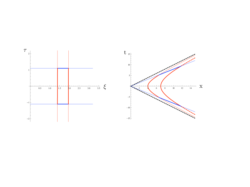
Figure 1: Wilson loop in Rindler (left) and Minkowski (right) coordinates

We compute the interaction energy for a rectangular loop with 2 of the 4 segments of the loop varying in time $\tau$ and $\xi,{\bf x}_{\perp}$ kept fixed while the other two segments are computed at fixed $\tau$. The sum $W_{0}$ of the two contributions from the integration along the $\tau$ axis can be carried out without specifying the segments in the spatial coordinates. Inserting (cf. Eq. (47))

$$D_{00}(\tau-\tau^{\prime},\xi,\xi^{\prime},{\bf x}_{\perp}-{\bf x}_{\perp}^{\prime})=\frac{a^{2}}{8i\pi^{2}}\frac{\cosh a(\tau-\tau^{\prime})}{\cosh a(\tau-\tau^{\prime})-\cosh\eta-i\delta}\,$$ (49)

into Eq.  (45) we find

$$W_{0}=\frac{e^{2}a^{2}}{8i\pi^{2}}\int_{0}^{T}ds\int_{0}^{T}ds^{\prime}\Big{[}\frac{\cosh a(s-s^{\prime})}{\cosh a(s-s^{\prime})-(1+i\delta)}-\frac{\cosh a(s-s^{\prime})}{\cosh a(s-s^{\prime})-(\cosh\eta+i\delta)}\Big{]}\,.$$ (50)

Here $\cosh\eta$ is given by (15) with the spatial coordinates $\xi^{(\prime)},{\bf x}_{\perp}^{(\prime)}$ of the vertices of the rectangle. Introducing $s\pm s^{\prime}$ as integration variables $W_{0}$ can be rewritten as

$$W_{0}=\frac{e^{2}a^{2}}{8i\pi^{2}}\int_{0}^{T}ds\Big{[}I_{0}(s,1+i\delta)-I_{0}(s,\cosh\eta+i\delta)\Big{]}\,,$$ (51)

with

$$I_{0}(s,\cosh\eta)=2\int_{0}^{s}ds^{\prime}\frac{\cosh as^{\prime}}{\cosh as^{\prime}-\cosh\eta-i\delta}=2s+\frac{2i\pi\cosh\eta}{a\sqrt{\sinh^{2}\eta+2i\delta}}$$

$$\cdot\left[1-\frac{i}{\pi}\left(\ln\frac{e^{as}-\cosh\eta-\sqrt{\sinh^{2}\eta+2i\delta}}{e^{as}-\cosh\eta+\sqrt{\sinh^{2}\eta+2i\delta}}+\ln\frac{1-\cosh\eta+\sqrt{\sinh^{2}\eta+2i\delta}}{\cosh\eta+\sqrt{\sinh^{2}\eta+2i\delta}-1}\right)\right].$$ (52)

The last step can be verified by differentiation. The contribution to the interaction energy $V$ of two oppositely charged sources can be extracted in the $T\to\infty$ limit from the two $s^{\prime}$ - independent terms in (52) (the integrals of the $s^{\prime}$ - dependent terms converge).

For large $T$, the integration along the spatial segments of the rectangle (the horizontal segments of the loop in Fig. 1) yields a $T$-independent term and does therefore not contribute to the interaction energy. The non-diagonal element $D_{01}$ gives rise to two space-time contributions to the Wilson loop which in the large $T$ limit become independent of the spatial coordinates and cancel each other. Thus we obtain the asymptotic value $\Sigma$ of the Wilson loop expressed in terms $\sigma$ (15)

$$\Sigma_{\pm}(\sigma)=\lim_{T\to\infty}\frac{1}{T}W_{0}=-\frac{e^{2}}{4\pi}a\coth\eta\big{[}1+\frac{i\eta}{\pi}\big{]}+U_{0}=V(\sigma)+U_{0}\,,$$ (53)

with the interaction energy

$$V(\sigma)=-\frac{e^{2}}{4\pi}a\frac{1+\sigma^{2}}{\sqrt{2\sigma^{2}+\sigma^{4}}}\Big{[}1+\frac{i}{\pi}\ln\frac{\sqrt{2\sigma^{2}+\sigma^{4}}+\sigma^{2}}{\sqrt{2\sigma^{2}+\sigma^{4}}-\sigma^{2}}\Big{]}\,.$$ (54)

The integration “constant” $U_{0}$ arises from the first term in (50) and represents the self-energy of the static charges. Regularizing the divergent integrals by point splitting, $U_{0}$ is given in terms of the proper distance in AdS₄ (cf. Eq. (15))

$$U_{0}=\frac{e^{2}a}{8\pi}\Big{(}\frac{1}{\sqrt{2}\delta\sigma(\xi)}+\frac{1}{\sqrt{2}\delta\sigma(\xi^{\prime})}+\frac{2i}{\pi}\Big{)}\,,\quad\delta\sigma^{2}(\xi^{(\prime)})=\frac{a^{2}}{2}\big{(}\delta\xi^{2}+e^{-2a\xi^{(\prime)}}\delta{\bf x}_{\perp}^{2}\big{)}.$$ (55)

Before discussing the properties of the “electrostatic” interaction and the comparison with the static scalar interaction we briefly describe a simple alternative method for calculating the interaction energy of two static charges. In analogy with the corresponding calculation for scalar fields (cf. Eqs. (28)-(32)) the current $j^{\mu}$ in Eq. (40) generated by two charges moving along the trajectories is parametrized as

$$\sqrt{|g|}j^{\mu}(v)=\sum_{i}e_{i}\int ds_{i}\frac{dv^{\mu}_{i}(s_{i})}{ds_{i}}\delta^{4}(v-v_{i}(s_{i}))\,,$$ (56)

resulting in the photon-charge vertex

$$S_{\text{int}}=\sum_{i}e_{i}\int ds_{i}A_{\mu}(v_{i}(s_{i}))\frac{dv_{i}^{\mu}}{ds_{i}}\,.$$ (57)

As for the scalar case (Eqs. (28)-(32)), the relevant quantity to be computed is the effective action which, for charges at rest in Rindler space, yields the sum of interaction and self energies

$$W_{\text{vc}} = \frac{1}{2}\sum_{i=1,2}e_{i}e_{j}\int ds_{i}\int ds_{j}D_{\mu\nu}\big{(}v_{i}(s_{i}),v_{j}(s_{j})\big{)}\frac{dv^{\mu}_{i}(s_{i})}{ds_{i}}\frac{dv^{\nu}_{j}(s_{j})}{ds_{j}}$$ (58)

$$= \frac{1}{2}\sum_{i,j=1,2}e_{i}e_{j}\int d\tau_{i}\int d\tau_{j}D_{00}\big{(}\tau_{i}-\tau_{j},\xi_{i},\xi_{j},{\bf x}_{i\,\perp}-{\bf x}_{j\,\perp}\big{)}\,,$$

where the propagators in different coordinates are obtained from each other by the corresponding coordinate transformations (cf. Eq. (47)). Unlike in the scalar case, for exchange of photons no factor renormalizes the coupling constants when changing from the proper $s_{i}$ to coordinate time $\tau$. We define the Fourier transform in time of the $00$-component of the propagator (Eq. (49)) by the limit

$$\tilde{D}_{00}(\omega,\xi,\xi^{\prime},{\bf x}_{\perp}) = \lim_{T\to\infty}\int_{-T}^{T}d\tau e^{i\omega\tau}D_{00}(\tau,\xi,\xi^{\prime},{\bf x}_{\perp})$$ (59)

$$= \frac{a^{2}\sin\omega T}{4i\pi^{2}\omega}+\frac{a}{4\pi}\coth\eta\Big{[}e^{-i\frac{\omega\eta}{a}}+\frac{2i\sin\frac{\omega\eta}{a}}{1-e^{-2\pi\frac{\omega}{a}}}\Big{]}\,,$$

and disregarding the (divergent) constant, for opposite charges $e=e_{1}=-e_{2}$, the result (54)

$$-e^{2}\tilde{D}_{00}(0,\xi,\xi^{\prime},{\bf x}_{\perp})=V(\sigma)\,,$$ (60)

is reproduced.

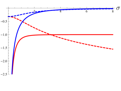
Figure 2: Real (solid) and imaginary (dashed) parts of the interaction energies $4\pi V_{sc}/a\kappa_{0}^{2}$ (33) and $4\pi V/ae^{2}$ (54) generated by scalar particle (blue) and photon (red) exchange respectively as a function of $\sigma$ (15).

In Fig. 2 are plotted real and imaginary parts of the interaction energy of two static charges in comparison with the interaction energy of two scalar sources. The distance which determines both scalar (33) and vector (54) interaction energies is the proper distance of the AdS₄ space and not of Rindler space, i.e., the static interaction energies generated by scalar particle and photon exchange are invariant under the scale transformation (17). At small distances where the effect of the inertial force is negligible both interaction energies display the familiar linear divergence in the real part and as in Minkowski space, vector and scalar exchange give rise to the same behavior. For small distances the imaginary part is constant and agrees with the constant in the finite temperature propagator (37) in Minkowski space

$$\lim_{\sigma\to 0}V(\sigma) = -\frac{e^{2}a}{4\pi}\Big{[}\frac{1}{\sqrt{2}\sigma}\big{(}1+\frac{3}{4}\sigma^{2}\big{)}+\frac{i}{\pi}\big{(}1+\frac{2}{3}\sigma^{2}\big{)}\Big{]}\,,$$ (61)

$$\lim_{\sigma\to 0}V_{\text{sc}}(\sigma) = -\frac{\kappa_{0}^{2}a}{4\pi}\Big{[}\frac{1}{\sqrt{2}\sigma}\big{(}1-\frac{1}{4}\sigma^{2}\big{)}+\frac{i}{\pi}\big{(}1+\frac{2}{3}\sigma^{2}\big{)}\Big{]}\,.$$ (62)

With increasing distance the inertial forces become important. They weaken both scalar and vector interaction energies and change completely the asymptotic behavior

$$\lim_{\sigma\to\infty}V(\sigma) = -\frac{e^{2}a}{4\pi}\Big{(}1+\frac{1}{2\sigma^{4}}+\frac{i}{\pi}\ln 2\sigma^{2}\Big{)},$$ (63)

$$\lim_{\sigma\to\infty}V_{\text{sc}}(\sigma) = -\frac{\kappa_{0}^{2}a}{4\pi}\frac{1}{\sigma^{2}}\Big{(}1+\frac{i}{\pi}\ln 2\sigma^{2}\Big{)}\,.$$ (64)

Significant differences in the asymptotics for scalar and vector exchange are obtained. Qualitative differences are observed for the imaginary part which vanishes asymptotically for scalar exchange and diverges logarithmically with $\sigma$ for photon exchange. Given the highly relativistic motion of the sources in Minkowski space, spin effects are expected to be important. Indeed the comparison of Eqs. (33) and (53) shows that the differences between scalar and vector exchange are due to the additional $\cosh\eta$ factor in (53) arising from the transformation of the propagator from Minkowski to Rindler space. In this context we also note the stronger asymptotic suppression of the “electrostatic” force in comparison to the force generated by scalar exchange. From the point of view of a Minkowski space observer (cf. Eq. (58)), cancellation between magnetic and electric forces generated by the spatial components of the current and by the charges respectively is to be expected.

Of particular interest is the behavior of the interaction energy if one of the sources approaches the horizon while the position of the other source is kept fixed. For

$$\xi_{h}\to-\infty,\quad\sigma^{2}\to\frac{1}{2}e^{-a(\xi_{h}+\xi)}\big{(}e^{2a\xi}+a^{2}({\bf x}_{\perp}-{\bf x}_{\perp}^{\prime})^{2}\big{)}\to\infty\,,$$ (65)

the interaction energies are given by

$$\lim_{\xi_{h}\to-\infty}V(\sigma) = -\frac{e^{2}a}{4\pi}\Big{(}1-i\frac{a(\xi_{h}+\xi)}{\pi}\Big{)}\,,$$ (66)

$$\lim_{\xi_{h}\to-\infty}V_{\text{sc}}(\sigma) = -\frac{\kappa_{0}^{2}a}{2\pi}e^{a(\xi_{h}+\xi)}\frac{1}{e^{2a\xi}+a^{2}({\bf x}_{\perp}-{\bf x}_{\perp}^{\prime})^{2}}\Big{(}1-i\frac{a(\xi_{h}+\xi)}{\pi}\Big{)}\,.$$ (67)

In both cases the interaction is dominated by the imaginary radiative contribution and no bound states are expected in this regime. We also find in analogy with the “no hair” theorem BEKE72 , BEKE98 , TEIT72 for Schwarzschild black holes that a scalar source close to the horizon cannot be observed asymptotically while vector sources are visible. Formally the difference arises from the running of the scalar coupling (32) to zero when approaching the horizon while the electromagnetic coupling remains constant. In detail the results for Rindler and Schwarzschild metrics are different. A significant improvement can be obtained by modifying the Rindler metric

$$ds^{2}=e^{2a\xi}(d\tau^{2}-d\xi^{2})-d{\bf x}_{\perp}^{2}\to e^{2a\xi}(d\tau^{2}-d\xi^{2})-\frac{1}{4a^{2}}\,d\Omega^{2}\,.$$ (68)

The dynamics in this space is very close to the dynamics in Rindler space unless the difference between the $S^{2}$ and $R^{2}$ matters. This is the case when deriving the “no hair” theorem where only the $l=0$ waves matter COWA71 .

III.2.2 Wilson loops of gauge fields in Weyl gauge

In the (covariant) Lorenz gauge only the $00$-component of the propagator contributes (cf. Eqs. (54) and (60)) which simplifies significantly the evaluation of the electrostatic interaction energy and by the same token hides the difference in origin of its real and imaginary parts. Separation of constrained and dynamical variables becomes manifest in Weyl gauge

$$A_{0}=0\,.$$

In this gauge one works with two unconstrained dynamical fields describing the photons and a longitudinal field constraint by the Gauß law. The gauge field is decomposed accordingly

$$A^{i}=\partial^{i}\chi+\hat{A}^{i}\,,$$ (69)

into the longitudinal component given by the scalar field $\chi$ and the transverse field satisfying

$$P^{i}_{\;j}\hat{A}^{j}=\hat{A}^{i}\,,\quad\text{with}\quad P^{i}_{\;j}=\delta^{i}_{\;j}+\partial^{i}\;\frac{1}{\Delta}\;\partial_{j},$$ (70)

and the Laplacian

$$\Delta=-\partial_{i}\partial^{i}=e^{-2a\xi}\big{(}\partial_{\xi}^{2}-2a\partial_{\xi}\big{)}+\partial^{2}_{\perp}\,.$$ (71)

Longitudinal and transverse fields are not coupled to each other. Their actions are given by

$$S_{\ell}[\chi]=-\frac{1}{2}\int d^{4}x\partial_{0}\partial_{i}\chi\partial_{0}\partial^{i}\chi\,,$$ (72)

and

$$S_{tr}[\hat{A}]=-\frac{1}{2}\int d^{4}x\partial_{0}\hat{A}_{i}\partial_{0}\hat{A}^{i}-\frac{1}{4}\int d^{4}x\sqrt{|g|}\,g^{ik}g^{jl}(\partial_{i}\hat{A}_{j}-\partial_{j}\hat{A}_{i})(\partial_{k}\hat{A}_{l}-\partial_{l}\hat{A}_{k})\,.$$ (73)

The Wilson loop expectation value factorizes into transverse and longitudinal contributions and the corresponding interaction energies (42) are additive. In Weyl gauge, the longitudinal contribution to the Wilson loop for a rectangle with one pair of its sides being parallel to the $\tau$ axis $(\tau_{0}=0\leq\tau\leq\tau_{1}=T)$ is given by

$$\oint_{\cal C}dx^{i}\partial_{i}\chi(\tau,\xi,{\bf x}_{\perp})=\int_{s_{0}}^{s_{1}}ds\frac{dx^{i}}{ds}\Big{(}\partial_{i}\chi(0,\xi(s),{\bf x}_{\perp}(s))-\partial_{i}\chi(T,\xi(s),{\bf x}_{\perp}(s))\Big{)}=\int d^{4}x\,\rho(x)\chi(x),$$

with

$$\rho(x)=\sum_{i,j=0,1}(-1)^{i+j+1}\delta(\tau-\tau_{i})\delta(\xi-\xi(s_{j}))\delta({\bf x}_{\perp}-{\bf x}_{\perp}(s_{j}))\,.$$

In terms of the Green’s function associated with the differential operators $\partial_{\tau}^{2}$ and the Laplacian (71)

$$\partial_{\tau}^{2}\frac{1}{2}|\tau|=\delta(\tau)\,,\quad\Delta G(\xi,{\bf x}_{\perp},\xi^{\prime},{\bf x}_{\perp}^{\prime})=\delta(\xi-\xi^{\prime})\delta({\bf x}_{\perp}-{\bf{x}}_{\perp}^{\prime})\,,$$ (74)

we find the following longitudinal contribution to the Wilson loop

$$W_{\ell}=-Te^{2}\big{[}G(\xi_{1},{\bf x}_{\perp\,1},\xi_{0},{\bf x}_{\perp\,0})-\frac{1}{2}\sum_{i=0,1}G(\xi_{i},{\bf x}_{\perp\,i},\xi_{i},{\bf x}_{\perp\,i})\big{]}\,.$$ (75)

The Green’s function $G$ has been calculated in LOY08 . It coincides with the real part of the static Lorenz gauge propagator (cf. Eq. (59))

$$G(\xi,{\bf x}_{\perp},\xi^{\prime},{\bf x}_{\perp}^{\prime})=\text{Re}\,\tilde{D}_{00}(0,\xi,\xi^{\prime},{\bf x}_{\perp}-{\bf x}_{\perp}^{\prime})\,,$$ (76)

and therefore up to irrelevant additive constants (cf. Eq. (54))

$$V(\sigma)=-e^{2}G(\xi_{1},{\bf x}_{\perp\,1},\xi_{0},{\bf x}_{\perp\,0})\,.$$ (77)

The transverse gauge field operators required for calculating the transverse contribution to the Wilson loop have been constructed in LOY08 with the $\xi$ component given by

$$\hat{A}_{1}(\tau,\xi,{\bf x}_{\perp})=e^{2a\xi}\int\frac{d\omega}{\sqrt{2\omega}}\frac{d^{2}k_{\perp}}{2\pi}\frac{k_{\perp}}{\omega}\Big{[}a_{1}(\omega,{\bf k}_{\perp})e^{-i\omega\tau+i{\bf k}_{\perp}{\bf x}_{\perp}}+\text{h.c.}\Big{]}\,\phi_{\omega,{\bf k}_{\perp}}(\xi,{\bf x_{\perp}})\,.$$ (78)

In order to avoid technical complications we assume the Wilson loop to be located in the $\tau$-$\xi$ plane. Applying the general expression (45) we obtain

$$W_{tr}(T,\xi_{1},\xi_{2},{\bf{0}}_{\perp})=e^{2}\int_{\xi_{1}}^{\xi_{2}}d\xi\int_{\xi_{1}}^{\xi_{2}}d\xi^{\prime}\{D^{W}_{11}(0,\xi,\xi^{\prime},{\bf{0}}_{\perp})-D^{W}_{11}(T,\xi,\xi^{\prime},{\bf{0}}_{\perp})\},$$ (79)

with the $11$ component of the Weyl gauge propagator

$$D_{11}^{W}(\tau,\xi,\xi^{\prime},{\bf x}_{\perp})=i\langle 0_{M}\big{|}T\big{[}\hat{A}_{1}(\tau,\xi,{\bf x}_{\perp})\hat{A}_{1}(0,\xi^{\prime},{\bf 0}_{\perp})\big{]}\big{|}0_{M}\rangle=-ie^{2a(\xi+\xi^{\prime})}\int_{0}^{\infty}\frac{d\omega}{\pi^{2}a}\sinh{\frac{\pi\omega}{a}}$$

$$\cdot\int\frac{d^{2}k_{\perp}}{(2\pi)^{2}}\frac{{k_{\perp}}^{2}}{{\omega}^{2}}(e^{-i\omega|\tau|}+\frac{2\cos{\omega\tau}}{e^{\frac{2\pi\omega}{a}}-1})K_{i\frac{\omega}{a}}\Big{(}\frac{k_{\perp}}{a}e^{a\xi}\Big{)}K_{i\frac{\omega}{a}}\Big{(}\frac{k_{\perp}}{a}e^{a\xi^{\prime}}\Big{)}e^{i\bf{k}_{\perp}\bf{x}_{\perp}}\,.$$ (80)

As above, the interaction energy is determined by the linearly divergent contribution to the Wilson loop in the large time limit $aT\gg 1$ and is generated by the thermal contribution in Eq. (80). We obtain for the transverse contribution to the Wilson loop

$$W_{tr}(T,\xi_{1},\xi_{2},{\bf{0}}_{\perp})=-iT\frac{e^{2}a}{4\pi^{2}}\big{(}\eta\coth{\eta}-1\big{)}\,,$$ (81)

which coincides with the imaginary part of $V(\sigma)$ (53) for $\eta=a(\xi_{1}-\xi_{2})$.

With the unambiguous separation of constraint and dynamical degrees of freedom in Weyl gauge, our result underlines the dynamical origin of the imaginary part of the Wilson loop in the large $T$ limit as opposed to the electrostatic origin of the real part. We essentially can apply now the arguments of Sect. II.3 concerning the imaginary part of the scalar propagator. The photons generated by an accelerated charge in Minkowski space are mapped into zero energy (transverse) photons in Rindler space. Though of zero energy, these transverse photons carry momentum and contribute therefore in a non-trivial way to the interaction energy. They propagate on the mass shell and their contribution to the interaction energy is therefore purely imaginary. Our derivation of the interaction energy of two static sources in Weyl gauge emphasizes the classical origin of the real part and the quantum mechanical origin of the imaginary part. Thereby it also confirms the relation of the zero modes in Rindler space generating the imaginary part with the Bremsstrahlung photons of the accelerated charge in Minkowski space.

III.3 Polyakov loop correlator

In numerical studies of gauge theories at finite temperature on the lattice an important quantity for characterizing the interaction energy of static charges is the correlation function of Polyakov loops JASM02 . These studies are carried out on a Euclidean lattice and have confirmed the existence of a transition in Yang-Mills theories from the confining to the deconfined phase. It would be of great interest to extend these studies to Rindler space and to follow the fate of the confined phase when approaching the horizon. In this paragraph we will calculate the Polyakov loop correlator in Rindler space with imaginary (Rindler) time (cf. Eq. (19)) which due to the acceleration is a periodic coordinate. Up to a multiplication with $i$, the “Euclidean” propagators are obtained from the real time propagators ((13) and (47)) by this change of the time coordinate. In particular the relevant component of the gauge field propagator (49) is given by

$$D_{00}^{E}(\tau_{E}-\tau^{\prime}_{E},\xi,\xi^{\prime},{\bf x}_{\perp}-{\bf x}_{\perp}^{\prime})=\frac{a^{2}}{8\pi^{2}}\frac{\cos a(\tau_{E}-\tau^{\prime}_{E})}{\cos a(\tau_{E}-\tau^{\prime}_{E})-\cosh\eta-i\delta}\,.$$ (82)

The periodicity in imaginary time expresses the similarity of acceleration and finite temperature. Unlike the temperature, the acceleration $a$ also appears together with the spatial coordinates. The Polyakov loop is defined by

$$P(e,\xi,{\bf x}_{\perp})=\exp\Big{\{}ie\oint d\tau_{E}A^{E}_{0}(\tau_{E},\xi,{\bf x}_{\perp})\Big{\}}\,,$$ (83)

and the Polyakov loop correlator associated with two static charges $e_{1,2}$ located at $\xi_{1,2},{\bf x}_{\perp\,1,2}$ is given by

$$C_{P}(\xi_{1},\xi_{2},{\bf x}_{\perp\,1},{\bf x}_{\perp\,,2}\big{)}=\langle 0_{M}|P(e_{1},\xi_{1},{\bf x}_{\perp\,1})\,P(e_{2},\xi_{2},{\bf x}_{\perp\,2})|0_{M}\rangle\,.$$ (84)

Written as a path integral, this correlation function is easily evaluated with the result

$$C_{P}(\xi_{1},\xi_{2},{\bf x}_{\perp\,1},{\bf x}_{\perp\,2}\big{)}=e^{-\frac{2\pi}{a}(f_{11}+f_{22}+2f_{12})}\,,$$ (85)

where the self and interaction energy contributions to the “free energy” $f_{ij}$ are given by (cf. Eq. (15))

$$f_{ij} = \frac{ae_{i}e_{j}}{32\pi^{3}}\int_{0}^{2\pi}ds\int_{0}^{2\pi}ds^{\prime}\frac{\cos(s-s^{\prime})}{\cosh\eta(\xi_{i},\xi_{j},{\bf x}_{\perp\,i}-{\bf x}_{\perp\,j})-\cos(s-s^{\prime})}$$ (86)

$$= \frac{ae_{i}e_{j}}{8\pi}\big{(}\coth\eta(\xi_{i},\xi_{j},{\bf x}_{\perp\,i}-{\bf x}_{\perp\,j})-1\big{)}\,.$$

Regularization by point splitting (cf. Eq. (55)) yields the self-energies

$$f_{ii}=\frac{e_{i}^{2}}{8\pi}\frac{1}{\sqrt{\delta\xi^{2}+e^{-2a\xi_{i}}\delta{\bf x}_{\perp}^{2}}}\,.$$ (87)

The interaction energy of the two charges

$$V_{P}\big{(}\xi_{1},\xi_{2},{\bf x}_{\perp\,1},{\bf x}_{\perp\,2}\big{)}=\frac{ae_{1}e_{2}}{4\pi}\Big{(}\coth\eta\big{(}\xi_{1},\xi_{2},{\bf x}_{\perp\,1}-{\bf x}_{\perp\,2}\big{)}-1\Big{)}\,,$$ (88)

agrees with the real part of the interaction energy obtained in the calculation of the Wilson loop in Lorenz gauge (54) and with the contribution from the longitudinal degrees of freedom (77). In agreement with the results of WALD70 concerning the equivalence of propagators defined in static space-time with either real or imaginary times, the Rindler space propagator (cf. Eq. (49)) can be reconstructed given the imaginary time propagator (cf. Eq. (82)). However, unlike in Minkowski space, this reconstruction may not work separately for single Fourier components such as the static component of the propagators. Apparently, the difference between imaginary and real time static propagators of the Maxwell field is due to the non-trivial (imaginary) contributions to the propagator from zero energy photons. For the case of Yang-Mills theories it remains to be seen how this missing information could be gained e.g. by studies of appropriate correlation functions.

III.4 Static gravitational interaction in Rindler space

To complete our discussion of static forces in Rindler space we sketch the calculation of the gravitational interaction of two point masses $M_{1,2}$ at rest in Rindler space. We apply the same method as above and start with the graviton propagator in Minkowski space which in harmonic gauge is, in terms of the scalar propagator (13), given by

$$D_{\mu\nu,\rho\sigma}=\chi_{\mu\nu,\rho\sigma}D(x,x^{\prime})\,,\quad\chi_{\mu\nu,\rho\sigma}=\frac{1}{2}\big{[}\eta_{\mu\rho}\eta_{\nu\sigma}+\eta_{\mu\sigma}\eta_{\nu\rho}-\eta_{\mu\nu}\eta_{\rho\sigma}\big{]}\,,$$ (89)

and $\eta_{\mu\nu}$ denotes the Minkowski space metric. With the relevant Rindler space tensor component of $\chi$,

$$\chi^{\prime}_{00,00}=\frac{1}{2}e^{2a(\xi+\xi^{\prime})}\cosh 2a(\tau-\tau^{\prime})\,,$$ (90)

the corresponding element of the propagator in Rindler space ordered according to the asymptotics in Rindler time $\tau$ reads

$$D^{(R)}_{00,00}(\tau,\xi,\xi^{\prime},{\bf x}_{\perp})=\frac{a^{2}}{4i\pi^{2}}(\cosh a\tau+\cosh\eta)\,e^{a(\xi+\xi^{\prime})}+(2\cosh^{2}\eta-1)\,e^{2a(\xi+\xi^{\prime})}\,D(\tau,\xi,\xi^{\prime},{\bf x}_{\perp})\,.$$ (91)

As for scalar (31) and vector exchange (58) we introduce also for graviton exchange the effective action

$$W_{\text{te}}=-G\sum_{i=1,2}M_{i}M_{j}\int ds_{i}\int ds_{j}D_{\mu\nu,\rho\sigma}\big{(}v_{i}(s_{i}),v_{j}(s_{j})\big{)}\frac{dv^{\mu}_{i}(s_{i})}{ds_{i}}\frac{dv^{\nu}_{i}(s_{i})}{ds_{i}}\frac{dv_{j}^{\rho}(s_{j})}{ds_{j}}\frac{dv^{\sigma}_{j}(s_{j})}{ds_{j}}\,,$$ (92)

which for the particles at rest in Rindler space represents their interaction and self-energies. As above (cf. Eq. (59)), for calculating the static interaction energy, we define the divergent $\tau$ integrals by integrating over a large but finite interval $[-T/2,T/2]$ and obtain from Eq. (92), after performing for the convergent terms the limit $T\to\infty$, the following expression for the static gravitational interaction energy

$$V_{\text{gr}}(\xi_{1},\xi_{2},{\bf x}_{\perp}-{\bf x}^{\prime}_{\perp})=-G\int d\xi d^{2}x_{\perp}d\xi^{\prime}d^{2}x^{\prime}_{\perp}T^{00}_{1}(\xi,{\bf x}_{\perp})T^{00}_{2}(\xi^{\prime},{\bf x}^{\prime}_{\perp})\tilde{D}^{(R)}_{00,00}(0,\xi,\xi^{\prime},{\bf x}_{\perp}-{\bf x}_{\perp}^{\prime})$$

$$=-GM_{1}M_{2}\Big{\{}\frac{a^{2}}{2i\pi^{2}}\Big{(}\frac{1}{a}\sinh\frac{aT}{2}+\frac{T}{2}\cosh\eta\Big{)}+\frac{a}{4\pi}\frac{2\cosh^{2}\eta-1}{\sinh\eta}\Big{[}1+\frac{i\eta}{\pi}\Big{]}\Big{\}}\,,$$ (93)

where $\eta=\eta(\xi_{1},\xi_{2},{\bf x}_{\perp\,1}-{\bf x}_{\perp\,2})$ (cf. Eq. (15)) and we have used the energy momentum tensor density of 2 particles at rest in Rindler space

$$T^{\mu\nu}_{i}(\xi,{\bf x}_{\perp})=M_{i}e^{-a\xi}\delta(\xi-\xi_{i})\delta({\bf x}_{\perp}-{\bf x}_{\perp\,i})\delta_{\mu\,0}\delta_{\nu\,0}\,.$$ (94)

We note that the interaction energies for the three cases considered (Eqs. (33), (53), (III.4)) depend only on the quantity $\eta$ (15) or equivalently $\sigma$ and are therefore invariant under the scale transformation (17). For scalar particle and graviton exchange the explicit $\xi,\xi^{\prime}$ dependent factors of propagators and vertices (cf. (27),  (28) and (92)) cancel each other while both photon propagator (49) and vertex (57) depend only on $\eta$

The terms divergent in the $T\to\infty$ limit are imaginary. They therefore satisfy the wave equation and are to be interpreted as the image of the gravitational radiation of the accelerated particles in Minkowski space. Both the imaginary contribution from the radiation and the real “static” gravitational interaction diverge with $\eta$. If evaluated in Minkowski coordinates, the source of these divergences of $W_{te}$ is not the propagator but the energy momentum tensor of uniformly accelerated particles

$$\tilde{T}^{\mu\nu}_{i} = M_{i}\frac{a}{x^{1}}e^{a\xi_{0}}\delta({\bf x}_{\perp}-{\bf x}_{\perp\,i})\delta\Big{(}x^{1}-\sqrt{t^{2}+a^{-2}e^{2a\xi_{0}}}\Big{)}$$ (95)

$$\cdot\Big{[}x^{1\,2}\delta_{\mu\,0}\delta_{\nu\,0}+x^{1}t(\delta_{\mu\,0}\delta_{\nu\,1}+\delta_{\mu\,1}\delta_{\nu\,0})+t^{2}\delta_{\mu\,1}\delta_{\nu\,1}\Big{]}\,.$$

The energy density as well as the density of the momentum in 1 direction and also the flux of the 1-component of the momentum in the 1 direction increase for sufficiently large positive or negative times like $|t|$. Thus the exponential increase of the graviton propagator with $\tau$ and with $\eta$ reflects the increase of the energy and momentum density in Minkowski space. Ultimately this increase invalidates the linearization of the Einstein equations and the backreaction on the gravitational field by the increasing energy-momentum tensor in Minkowski space or equivalently by the increasing propagator in Rindler space has to be taken into account.

IV Hydrogen-like systems and the stability of matter in Rindler space

IV.1 Non-relativistic limit of accelerated atoms

As an application of the formal development we will address in this section the issue of stability of matter under uniform acceleration. The radical change of the dispersion relation between energy and momentum of elementary particles makes it very unlikely that matter as observed in Minkowski space will be formed in an accelerated frame. We will address this issue in a study of the effect of acceleration on hydrogen-like atoms consisting of an infinitely heavy, pointlike nucleus of charge $Z$ and a single electron. We will present evidence that the atomic structure is destroyed by uniform acceleration.

The acceleration $a$ will be chosen to be small in comparison to the electron mass $m_{e}$ in order to keep the electron motion in the rest frame of the nucleus non-relativistic. Furthermore, to simplify the calculation we treat the electron as a scalar particle. Keeping only the coupling between electron and nucleus via $A_{0}$, the approximate Lagrangian is

$${\cal L}=\sqrt{|g|}\;(\partial_{\mu}\phi\partial^{\mu}\phi^{\dagger}-m^{2}\phi\phi^{\dagger})-ie^{2}\big{(}\tilde{D}_{00}(0,\xi+\xi_{Z},\xi_{Z},{\bf x}_{\perp})+U_{0}^{Z}(\xi+\xi_{Z},\xi_{Z},{\bf x}_{\perp})\big{)}$$

$$\hskip 15.6491pt\cdot\;\Big{[}\phi^{\dagger}(\xi,{\bf x}_{\perp})\;\dot{\phi}(\xi,{\bf x}_{\perp})-\dot{\phi}^{\dagger}(\xi,{\bf x}_{\perp})\;\phi(\xi,{\bf x}_{\perp})\Big{]}\,,$$ (96)

with the coordinates $\{\xi_{Z}\,,{\bf x}_{\perp\,Z}=0\}$ and $\{\xi+\xi_{Z},{\bf x}_{\perp}\}$ denoting the position of the nucleus and the electron respectively and with $\tilde{D}_{00}$ given in Eqs. (54) and (60). Besides the interaction energy, the Lagrangian also contains the lowest order self energy (cf. Eq. (55))

$$U_{0}^{Z}(\xi+\xi_{Z},\xi_{Z},{\bf x}_{\perp})=\frac{e^{2}a}{8\pi}\Big{(}\frac{1}{\sqrt{2}\delta\sigma(\xi+\xi_{Z})}+\frac{Z^{2}}{\sqrt{2}\delta\sigma(\xi_{Z})}+\frac{i(1+Z^{2})}{\pi}\Big{)}\,.$$ (97)

With the Ansatz

$$\phi(\tau,\xi,{\bf x}_{\perp})=e^{-i\omega\tau}\varphi(\xi,{\bf x}_{\perp})\,,$$

the stationary wave equation reads

$$\Big{[}-\omega^{2}-\partial^{2}_{\xi}+(-\partial^{2}_{\perp}+m^{2})\,e^{2a(\xi_{Z}+\xi)} + 2\omega\,\{Ze^{2}\tilde{D}_{00}(0,\xi+\xi_{Z},\xi_{Z},{\bf x}_{\perp})$$ (98)

$$+ U_{0}^{Z}(\xi+\xi_{Z},\xi_{Z},{\bf x}_{\perp})\}\Big{]}\;\varphi(\xi,{\bf x}_{\perp})=0\,.$$

In the non-relativistic approximation the energy is dominated by the mass term

$$\omega^{2}=(m+E)^{2}e^{2a\xi_{Z}}\approx(m^{2}+2mE)e^{2a\xi_{Z}}\,,$$ (99)

and the Hamiltonian associated with the wave equation (98) is given by (cf. Eq. (54))

$$H=-\frac{1}{2m}\big{(}e^{-2a\xi_{Z}}\partial_{\xi}^{2}+e^{2a\xi}\partial_{\perp}^{2}\big{)}+e^{-a\xi_{Z}}\big{(}V(\sigma)+U_{0}^{Z}\big{)}+\frac{m}{2}\big{(}e^{2a\xi}-1\big{)}\,,$$ (100)

with $E$ denoting an eigenvalue of $H$. In comparison to the Hamiltonian in Minkowski space both potential and kinetic energies are significantly modified. Only by the requirement of weak acceleration, i.e. if $a$ is mall in atomic units,

$$a\rho_{B}\ll 1\,\quad\text{with the Bohr radius}\quad\rho_{B}=\frac{1}{mZ\alpha}\,,$$ (101)

the connection of $H$ to the Minkowski space Hamiltonian becomes transparent. In general, the macroscopic coordinate of the nucleus $\xi_{Z}$ is large on this scale. In this weak acceleration limit, we replace $V(\sigma)$ by the leading term in the expansion (61), rescale the variable $\xi$ and the regulator $\delta\xi$ (cf. Eq. (97))

$$z=\xi e^{a\xi_{Z}}\,,\quad\delta z=\delta\xi e^{a\xi_{Z}}\,,$$ (102)

and introduce the local acceleration (cf. RIND01 )

$$\quad a_{Z}=ae^{-a\xi_{Z}}\,.$$ (103)

The resulting Hamiltonian reads

$$H=H_{0}+W=-\frac{1}{2m}\Delta-\frac{Z\alpha}{\sqrt{z^{2}+{\bf x}_{\perp}^{2}}}+ma_{Z}z+W,$$ (104)

with (cf. Eq. (97))

$$W=e^{-a\xi_{Z}}\big{(}i\,\text{Im}V(\sigma)+U_{0}^{Z}\big{)}=\frac{(Z^{2}+1)e^{2}}{8\pi\sqrt{\delta z^{2}+\delta{\bf x}_{\perp}^{2}}}+\frac{ia_{Z}e^{2}}{8\pi^{2}}\Big{(}(Z-1)^{2}-\frac{2\,Z}{3}a_{Z}^{2}(z^{2}+{\bf x}_{\perp}^{2})\Big{)}\,.$$ (105)

In the weak acceleration limit, the real part of the sum of the electrostatic self energies of the electron and the nucleus is a complex constant independent of $\xi$ and can be dropped.

IV.2 The imaginary part of the Coulomb interaction

The imaginary part of the Hamiltonian (104) reflects the presence of on-shell propagating zero energy photons. The leading term is the self energy of the total charge $Z-1$. It increases linearly with the local acceleration $a_{Z}$ and expresses the instability of the bare source towards decay into source and zero energy photons. Thus a static charge in Rindler space is accompanied by on-shell zero energy photons. This “cloud” of photons is nothing else than the image in Rindler space of the Bremsstrahlung photons generated by the accelerated charge in Minkowski space.

In a system of two oppositely charged sources ($Z=1$) the imaginary part of self energy and interaction energy contributions cancel each other for small distances (cf. Eq. (105)). In this limit where the opposite charges neutralize each other, no Bremsstrahlung is generated in Minkowski space and no zero energy photons in Rindler space. Beyond this limit and due to the peculiar energy-momentum dispersion relation, a new phenomenon appears. For values of the acceleration of the order of the inverse distance of the two charges, momentum is transferred by the exchange of zero energy photons. As shown in Fig. 2, the corresponding imaginary part of the interaction energy increases logarithmically with the distance $\sigma$ of the two charges giving rise to a long range (imaginary) force between the static charges. With regard to conceptual issues concerning signatures of the Unruh effect, a detailed study of the consequences of this force for the dynamics of electromagnetically bound systems, e.g., the hydrogen atom, would be of interest. Simple answers can be obtained only in the limit of small acceleration (Eq. (101)). In this limit perturbation theory applied to $\text{Im}W$ yields the width of the hydrogen states induced by the acceleration

$$\Gamma_{n\ell}=\frac{e^{2}}{6\pi^{2}}a_{Z}^{3}\langle n\ell|\,r^{2}\,|n\ell\rangle=\frac{e^{2}}{12\pi^{2}}a^{3}_{Z}\rho_{B}^{2}\big{[}5n^{2}+1-3\ell(\ell+1)\big{]}\,.$$

The inverse of $\Gamma$ is the time it takes a bare hydrogen atom to get dressed by zero-energy photons. For this dressing to occur on the atomic time scale, the acceleration $a_{Z}$ has to be of the order of $m\alpha$ and therefore larger by a factor of $1/\alpha^{2}$ than typical atomic accelerations. With “macroscopic” accelerations such as the acceleration at the horizon of a black hole, the time it takes to build up the photon cloud is of the order of the age of the universe.

Due to the dependence of $\text{Im}\,W$ on the electron coordinate, initial and final hydrogen states are not necessarily identical but it appears that energy conservation forbids such a transition. On the other hand, considering the corresponding process in Minkowski space, nothing forbids for instance emission of a Bremsstrahlung photon by an infinitely heavy proton followed by absorption of the (on-shell) photon by the electron and thereby producing an excited state of the hydrogen atom. In Rindler space the on-shell photon is mapped into a zero mode and therefore the excitation of the atom occurs without energy transfer. Thus ground and excited states must be degenerate which in turn suggests that the initial state must be an ionized state. In the following more detailed calculations we will show that this indeed is the case.

IV.3 Decay of uniformly accelerated hydrogen-like atoms

In this section we are discussing the effect of the inertial force in hydrogen like atoms which are at rest in Rindler space. In particular we will discuss the instability of the atomic states due to ionization by the inertial force described by the term linear in $z$ of the Hamiltonian (104). For the following discussion the contribution $W$ to the Hamiltonian (104) is irrelevant and will be neglected. The Hamiltonian $H_{0}$ is the standard non-relativistic Hamiltonian of hydrogen-like systems complemented by the dipole term $ma_{Z}z$ which is the small $z$ limit of the inertial force $m^{2}e^{2a\xi}$ in the wave-equation (6). As required by the equivalence principle, to leading order in the acceleration $a$, this additional term appears as an external homogeneous gravitational field.

Although of different dynamical origin, the Hamiltonian $H_{0}$ coincides, after reinterpretation of the constants, with that of a hydrogen-like system in the presence of an external, constant electric field. For the analysis of the spectrum we employed the techniques developed for the description of the Stark effect BESA57 , HIOS96 , and carried out the computation of the shift in the spectrum and of the lifetime of the ground state by using parabolic coordinates.

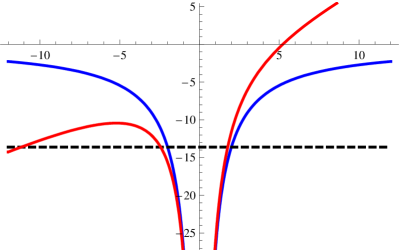
Figure 3: Coulomb potential (blue) and sum of Coulomb and inertial potential (red) in eV along an axis through the origin tilted with respect to the $z$-axis by $60^{\circ}$ with $a\rho_{B}\approx 10^{-7}$ with the distance to the origin given in units of the Bohr radius.

The nature of the spectrum is determined by the interplay between the inertial force and the electrostatic force (cf. Eq. (54)) as is demonstrated in Fig. 3. The relative strength of inertial and electrostatic interactions is given by the parameter

$$\gamma=\frac{a_{Z}}{mZ^{3}\alpha^{3}}\,,$$ (106)

which is the ratio between the local acceleration $a_{Z}$ and the radial acceleration of the electron at the Bohr radius.

When turning on acceleration the first signatures of the presence of inertial forces are changes in the spectrum. The ground state energy of the hydrogen atom is modified in second order perturbation theory (quadratic Stark effect). For $\gamma=8\cdot 10^{-3}$, i.e. $a_{Z}\approx 7\cdot 10^{-20}$ m s^-2, the shift $\Delta E$ of the ground state energy $E_{0}$ is given by

$$\frac{\Delta E}{E_{0}}=\frac{9}{2}\gamma^{2}=0.00029\,.$$ (107)

Since the leading term vanishes in lowest order perturbation theory, corrections to the Hamiltonian $H_{0}$ (104) proportional to $a_{Z}^{2}$ have to be considered. The dominant contribution comes from the expansion of the inertial force in Eq. (100), $\Delta_{2}H=ma^{2}_{Z}z^{2}$. In comparison to (107), the resulting shift of the ground state energy is suppressed by two powers of $\alpha$

$$\frac{\Delta_{2}E}{\Delta E}=-\frac{4}{9}\alpha^{2}\,.$$ (108)

Corrections to the Coulomb interaction (cf. Eqs. (100), (61)) are suppressed by still higher powers of $\alpha$.

With increasing acceleration we also have to account for the decay of the atom induced by the inertial force. As Fig. 3 shows, strictly speaking no stable hydrogen bound state exists whatever the non vanishing value of the acceleration may be, thereby confirming the above conjecture that existence of the imaginary part together with energy conservation in Rindler space is not compatible with the existence of atomic bound states. If on the other hand we assume that the acceleration has not been present for infinite time i.e. the atom has not been close to a black hole infinitely long, the lifetime of the atom is a useful quantity to characterize the effect of the acceleration on the stability of matter. In such a case, the atom decays by tunneling of the electron through the potential barrier. With decreasing $\gamma$ the potential energy approaches the Coulomb potential and the lifetime of the metastable state tends to infinity. Above a critical value $\gamma=\gamma_{c}$ where the two turning points coalesce, a meaningful definition of a metastable state becomes impossible. In this regime the inertial force is dominant and no bound states are formed.

Within the formulation in terms of parabolic coordinates the critical value can be computed with the results

$$\gamma_{c}=2(3+\sqrt{7})/(2+\sqrt{7})^{3}=0.11\,,$$ (109)

and the lifetime of the ground state of hydrogen-like systems can be estimated by calculating the tunneling probability in the WKB approximation. The resulting expression for the width reads

$$\Gamma=|E_{0}|\frac{8}{\gamma}e^{-\frac{2}{3\gamma}}\,.$$ (110)

The decay rate of the hydrogen atom is determined by the tunneling probability of the electron $\sim\gamma^{-1}\exp\{-2/3\gamma\}$ and the frequency $\sim|E_{0}|$ with which the electron reaches the classically forbidden region. With the above choice of $8\cdot 10^{-3}$ for the parameter $\gamma$ the lifetime of the hydrogen atom is of the order of the age of the universe, while, when increasing the acceleration by a factor of 14 to reach the critical value $\gamma_{c}$, the width is about $2\%$ of the ground state energy and no metastable state is formed.

IV.4 Instability of matter

The decrease of the lifetime of the hydrogen atom is a consequence of the dependence of the acceleration on the position of the nucleus and is another signature of the spatial variation of the Tolman temperature appearing for instance in the energy momentum tensor of photons in Rindler space CADE77 , SCCD81 . As a consequence, in an accelerated “rocket”, with the local acceleration, also the degree of ionization varies within the rocket as described by $a_{Z}$ (Eq. (103)). For interpretation of these results in terms of an ensemble of atoms stationary near the horizon of a black hole, it is convenient to introduce the (proper) distance of the nucleus to the horizon which, for given $\xi_{Z}$, reads (cf. Eq. (16), (103))

$$d_{H}(\xi_{Z})=\frac{1}{a}e^{a\xi_{Z}}=\frac{1}{a_{Z}}\,.$$ (111)

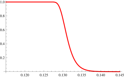
Figure 4: Ionization probability of hydrogen atoms as a function of the distance to the horizon (111) of a black hole.

In Fig. 4 is shown the probability that an ensemble of hydrogen atoms has been ionized since the big bang as a function of the proper distance from the horizon e.g. from a Schwarzschild black hole. We note that only the value of the local acceleration $a_{Z}$ matters (cf. Eqs. (106), (110)) and therefore the curve shown in Fig. 4 is independent of the acceleration $a$, i.e. of the mass of the black hole. The transition from atoms to ions happens at a distance of about $10^{-4}$ m within an interval of the order of $10^{-5}$ m.

In extending these arguments to other forms of matter we find that heavy atoms (cf. Eqs. (106), (110)) are ionized by the inertial force at a distance from the horizon of the order of $10^{-10}$ m. Using similar qualitative arguments based on the approximate identity of inertial and the strong force in the region of “ionization”, ejection of a nucleon from the nucleus by acceleration is estimated to occur at a distance to the horizon of the order of $10^{-13}$ m. However, in this case as well as for heavy atoms, the identification of the interaction in accelerated and inertial frames may become problematic. Since we expect the strong interaction to be reduced by the inertial force as is the case for electrostatic interactions, these distances to the horizon are most likely underestimated. As for the atoms, no bound states of nucleons can exist irrespective of the details of the nuclear force provided the acceleration has lasted for an infinitely long time. In turn, tunneling processes may also be important for the instability of nuclei.

As far as the stability of elementary particles are concerned which are subject to an infinitely long lasting acceleration, related arguments can be put forward which indicate that also in the presence of interactions their properties in Rindler space will remain to be quite different from those in Minkowski space. For illustration we consider a self-interacting scalar field which, depending on the interaction, may involve mass generation accompanied by spontaneous symmetry breakdown. The Rindler space Hamiltonian of a self interacting scalar field is given by (cf. (10))

$$H=\frac{1}{2}\int d\xi d^{2}x_{\perp}\big{\{}\pi^{2}+(\partial_{\xi}\phi)^{2}+e^{2a\xi}\big{(}(\boldsymbol{\partial}_{\perp}\phi)^{2}+V(\phi)\big{)}\,\big{\}}$$ (112)

with $V$ chosen such that the minimum of $V$ occurs for $\phi=\pm\phi_{0}\neq 0$. The expectation value $\phi_{0}$ of the scalar field generated by the self interaction obviously remains the same after carrying out the coordinate transformation from Minkowski to Rindler space (cf. UNRU84 for a discussion within the path integral approach). The implications of the symmetry breaking in Rindler space are not as obvious as in Minkowski space. Symmetry breaking with mass generation does not leave signatures in the spectrum of the effective Hamiltonian in Rindler space. Furthermore as for non-interacting theories, in the presence of accelerated sources scalar particle production by acceleration in Minkowski space gives rise to on-shell zero energy particles present in Rindler space. A cloud of scalar on-shell particles is present for both massive and massless particles. On the other hand, we also cannot invoke the restoration of symmetry, when heating the system, as an argument for a phase transition by increase of the acceleration $a$. A change in $a$ not only changes the temperature but also the Hamiltonian (112). Thus it is not obvious that a non-vanishing $\phi_{0}$ also implies a change from the symmetric to the symmetry broken phase in the whole of Rindler space. Rather it seems plausible that, in analogy to the transition of an ensemble of atoms in Fig. 4, locally either the broken or the restored symmetry is realized depending on the distance from the horizon. To be more specific we consider the standard $\phi^{4}$ potential and expand it around the minimum at $\phi=\phi_{0}$

$$V(\phi)=V(\varphi,\phi_{0})=\frac{\lambda}{8}\phi^{2}(\phi^{2}-2\phi_{0}^{2})\approx-\frac{\lambda}{8}\phi_{0}^{4}+\frac{m^{2}}{2}\varphi^{2}\,,\quad m^{2}=\lambda\phi^{2}_{0}.$$ (113)

Although formally the minimum in the potential energy $V(\phi)$ is attained at $\phi=\phi_{0}$ independent of the value of $\xi$, it is also plausible that the relevance of this minimum depends on the value of $\xi$. It has been argued PADM10 that, for sufficiently small $\xi$, the potential $V(\phi)$ together with the transverse kinetic term can be neglected resulting in a reduction to a non-interacting massless 1+1 dimensional field theory. Here we give a rough estimate of the value of $\xi$ where the effect of the potential $V(\phi)$ becomes negligible by equating the fluctuations in the energy density including those generated by the transverse motion

$$\epsilon(\xi)=e^{-2a\xi}\langle 0_{M}|:{\cal H}(\xi,{\bf x}_{\perp}):|0_{M}\rangle=\frac{e^{-2a\xi}}{2}\langle 0_{M}|:\pi^{2}+(\partial_{\xi}\varphi)^{2}+e^{2a\xi}\big{(}(\boldsymbol{\partial}_{\perp}\varphi)^{2}+m^{2}\varphi\big{)}:|0_{M}\rangle\,.$$ (114)

with the change in energy density associated with the local breaking of the reflection symmetry $\phi\to-\phi$

$$\epsilon(\xi)\approx\frac{\lambda}{8}\phi_{0}^{4}\,.$$ (115)

The expectation value $\epsilon(\xi)$ is taken in the Minkowski space vacuum with the operator ${\cal H}(\xi,{\bf x}_{\perp})$ being normal ordered with respect to the Rindler space vacuum. Inserting the normal mode expansion (9) and carrying out the ${\bf k}_{\perp}$ integration (cf. RG65 ) we obtain for the energy density as a function of the distance to the horizon $d_{H}=e^{a\xi}/a$ (cf. Eq. (111))

$$\epsilon(d_{H})=\frac{m^{2}}{4\pi^{3}d_{H}^{2}}\int_{0}^{\infty}d\chi e^{-\pi\chi}\Big{\{}(\chi^{2}+1)\Big{[}K_{1+i\chi}(md_{H})K_{1-i\chi}(md_{H})-\big{(}K_{i\chi}(md_{H})\big{)}^{2}\Big{]}$$

$$-\frac{1}{2}K_{i\chi}(md_{H})\Big{[}md_{H}K^{\prime}_{i\chi}(md_{H})-K_{i\chi}(md_{H})\Big{]}\Big{\}},$$ (116)

where $K^{\prime}_{i\chi}$ denotes the derivative with respect to the argument. Numerical evaluation of this integral shows that for $md_{H}\leq 0.2,$ the energy density agrees within 10% or less with the $m=0$ limit which can be calculated in closed form

$$\epsilon(d_{H})\approx\frac{11}{480\pi^{2}d_{H}^{4}}\,.$$ (117)

The energy densities associated with the symmetry breakdown and with the fluctuations are of the same order of magnitude for the following value of the distance to the horizon

$$d_{H}\approx\Big{(}\frac{11}{60\,\pi^{2}\lambda}\Big{)}^{\frac{1}{4}}\frac{1}{\phi_{0}}\,.$$ (118)

Identifying the parameters $\lambda$ and $\phi_{0}$ with those of the Higgs potential of the standard model (with the Higgs mass $100\,\text{GeV}\leq m\leq 250\,\text{GeV}$), Eq. (118) yields, in qualitative agreement with the numerical evaluation of Eqs. (115) and (116), $d_{H}\approx(4\pm 1)\cdot 10^{-19}$ m, i.e., we expect that at these or smaller distances the presence of a non-vanishing expectation value of the scalar field will be irrelevant. The expression (117) for the variation in the energy density can also be interpreted as due to the spatial variation of the Tolman temperature

$$T_{\text{Tolman}}=\frac{1}{2\pi d_{H}}\,.$$ (119)

Up to numerical factors, the energy density (117) is that of a massless scalar field in 3+1 dimensions at the temperature $T=T_{\text{Tolman}}$. The value $T_{\text{Tolman}}\approx 80$ GeV is of the same order of magnitude as the critical temperature of the electroweak phase transition.

V Conclusions

The focus of our studies of quantum fields in Rindler space has been on the forces which are generated by exchange of massless bosons and are acting between sources at rest in Rindler space. We have presented detailed results for exchange of scalar particles, photons and gravitons. In comparison to Minkowski space, the most striking difference of the interaction energies is the appearance of a non-trivial imaginary part in Rindler space. Unlike the (classical) real part of the interaction energy, the imaginary part is of quantum mechanical origin. The difference between real and imaginary contributions can be lucidly illustrated for photon exchange. In Weyl gauge, longitudinal and transverse degrees of freedom are cleanly separated with the longitudinal field determining the real and the transverse photons the imaginary part.

In contrast to the universal $1/r$ behavior in Minkowski space, the real part of the interaction energies in Rindler space exhibits significant differences for the three cases considered. Independent of the spin of the exchanged particles is only the behavior of the forces at short distances where inertial forces are negligible and the leading terms agree with the Minkowski space result. For large separations of the sources, the real part of the interaction energy of scalar sources is suppressed and the electrostatic interaction energy approaches a non-vanishing constant while a divergence is encountered for gravitational sources. Significant differences also appear when approaching the horizon akin to the differences which, in the context of the “no-hair” theorem, have been obtained close to the horizon of a Schwarzschild black hole BEKE72 , BEKE98 , TEIT72 .

The existence of an imaginary contribution to the interaction energy is a direct consequence of the peculiar degeneracy of the spectrum of Rindler space particles and is therefore of the same origin as the one-dimensional density of states appearing in the energy-momentum tensor of scalar or vector fields CADE77 , SCCD81 . The degeneracy is a consequence of the invariance of the Rindler space Hamiltonian under scale transformations as is the scale invariance of the static interaction energies. Of particular relevance for the static interactions is the degeneracy of the zero energy sector of the Rindler particles. The degeneracy is characterized by the values of the 2 momentum components transverse to the direction of the acceleration. The imaginary part is generated by emission, on-shell propagation and absorption of zero energy Rindler particles and is directly related to the (zero energy) particle creation and annihilation rates in Rindler space. This result, together with the connection of “radiation” in Rindler and Minkowski spaces HIMS921 , HIMS922 , REWE94 , implies that the imaginary part of the interaction energy in Rindler space is given by the rate of particle production of a uniformly accelerated charge in Minkowski space, measured by the Rindler time. Thus consistency between the radiation observed in Minkowski space and the zero energy radiation in Rindler space is established by the existence of a non-trivial zero energy sector which in turn requires a symmetry which guarantees the degeneracy. Seen from this point of view it may not come as a surprise that the symmetry under appropriately generalized scale transformations persists LOY08 for massive particles and guarantees consistency between Rindler and Minkowski space formulations also in this case. While negligible for small separations of the two sources, the imaginary contribution dominates the force at large distances for scalar particle and photon exchange. As the real part, also the imaginary part of the gravitational interaction is divergent. The counterpart of this divergence of the static graviton propagator in Rindler space is the divergence of the energy momentum tensor of the “eternally”, uniformly accelerated mass point in Minkowski space. This divergence indicates that the implicit assumption of a negligible backreaction on the gravitational field is invalid.

The weakening of the interaction for scalar particle and photon exchange as well as the appearance of a non-trivial imaginary contribution point to instability of matter in Rindler space. We have confirmed this instability in a calculation of the rate of ionization of hydrogen atoms at rest as a function of the distance from the horizon or equivalently of the Tolman temperature. Similar arguments point to the instability of nuclear matter which will set in at significantly smaller distances to the horizon. In this hierarchy of instability one may also expect, at still smaller distances, instability of the phases of matter determined by the dynamics of quantum fields. Within the context of a self-interacting scalar field we have shown that the strength of the fluctuations increases when approaching the horizon and we have determined the distance where the fluctuations and the mean field generated by symmetry breaking contribute equally to the energy density. At still smaller distances, most likely the expectation value of the scalar field becomes irrelevant for the dynamics. Using parameters of the standard model, the corresponding Tolman temperature has been found to be of the same order of magnitude as the temperature of the electroweak phase transition. Of interest in this context is the issue of a possible confinement-deconfinement transition when approaching the horizon. As in Minkowski space, this issue most likely has to be settled in numerical simulations. The strong force will have to be determined in calculations of the Polyakov loop correlation functions on a lattice in Rindler space with imaginary time. As in the electrostatic case the interaction energy determined in this way will be a real quantity. Whether confinement in Rindler space implies a vanishing imaginary contribution to the force or the imaginary part can be reconstructed, on the basis of the numerically determined spectrum and correlation functions, has to be clarified.

References

- (1) S. A. Fulling, Phys. Rev. D 7, (1973), 2850
- (2) D. G. Boulware, Phys. Rev. D 11, (1975), 1404
- (3) P. C. W. Davies, J. Phys. A 8, (1975), 609
- (4) W. G. Unruh, Phys. Rev. D 14, (1976), 870
- (5) W. D. Sciama, P. Candelas and D. Deutsch, Adv. in Phys. 30, (1981), 327
- (6) A. Higuchi, G. E. A. Matsas and D. Sudarsky, Phys. Rev. D 45, (1992), R3308
- (7) A. Higuchi, G. E. A. Matsas and D. Sudarsky, Phys. Rev. D 46, (1992), 3450
- (8) H. Ren and E. J. Weinberg, Phys. Rev. D 49, (1994), 6526, [arXiv:hep-th/9312038]
- (9) L. C. B. Crispino, A. Higuchi and G. E. A. Matsas, Rev. Mod. Phys. 80, (2008), 787, [arXiv:gr-qc/0710.5373]
- (10) W. G. Unruh and N. Weiss, Phys. Rev. D 29, (1984), 1656
- (11) R. Passante, Phys. Rev. A 57, (1998), 1590
- (12) R. Müller, Phys. Rev. D 56, (1997), 953
- (13) D. A. T. Vanzella and G. E. A. Matsas, Phys. Rev. D 63, (2000), 014010, [arXiv:hep-th/0002010]
- (14) F. Lenz, K. Ohta and K. Yazaki, Phys. Rev. D 78, (2008), 065026, [arXiv:hep-th/0803.2001]
- (15) W. Rindler, Relativity, Special, General and Cosmological, Oxford University Press, 2001
- (16) W. Trost and H. Van Dam, Phys. Lett. B 71, (1977), 149 and Nucl. Phys. B 152, (1979), 442
- (17) J. S. Dowker, Phys. Rev. D 18, (1978), 1856
- (18) S. M. Christensen and M. J. Duff, Nucl. Phys. B 146, (1978), 11
- (19) B. Linet, [arXiv:gr-qc/9505033]
- (20) N. F. Svaiter ans C. A. D. Zarro, Class. Quant. Grav. 25, (2008), 095008
- (21) P. Candelas and D. J. Raine, J. Math. Phys. 17, (1976), 2101
- (22) I. S. Gradshteyn and I. M. Ryzhik, Table of Integrals, Series and Products, Academic Press 1965
- (23) A. Erdelyi, W. Magnus, F. Oberhettinger and F. G. Tricomi, Higher Transcendental Functions, Vol. I, McGraw Hill 1953
- (24) P. G. Grove, Class. Quant. Grav. 3, (1986), 801
- (25) S. Massar, R. Parentani and R. Brout, Class. Quant. Grav. 10, (1993), 385
- (26) W. G. Unruh, Phys. Rev. D 46, (1992), 3271
- (27) B. L. Hu and A. Raval, [arXiv:quant/ph 0012134]
- (28) J. Baez & J. P. Muniain, Gauge Fields, Knots and Gravity, World Scientific, 1994
- (29) J. Smit, Introduction to Quantum Fields on a Lattice, Cambridge University Press, 2002
- (30) J. D. Bekenstein, Phys. Rev. Lett. 28, (1972), 452
- (31) J. D. Bekenstein, Black Holes: Classical Properties, Thermodynamics and Heuristic Quantization, in: Cosmology and Gravitation, Atlanticsciences, M. Novello (Ed.) p. 1
- (32) C. Teitelboim, Phys. Rev. D 5, (1972), 2951
- (33) J. M. Cohen and R. M. Wald, J. Math. Phys. 12, (1971), 1845
- (34) M. Wald, Commun. Math. Phys. 70, (1979), 221
- (35) H. A. Bethe and E. E. Salpeter, Quantum mechanics of one- and two-electron atoms, Springer Verlag, 1957
- (36) K.-I. Hiraizumi, Y. Y. Ohshima and H. Suzuki, Phys. Lett. A 216, (1996), 117
- (37) P. Candelas and D. Deutsch, Proc. R. Soc. Lond. A 354, (1977), 79
- (38) T. Padmanabhan, Rep. Prog. Phys. 73, (2010), 046901 [arXiv:gr-qc/0911.5004]