Incentive Games and Mechanisms
for Risk Management

Abstract

Incentives play an important role in (security and IT) risk management of a large-scale organization with multiple autonomous divisions. This paper presents an incentive mechanism design framework for risk management based on a game-theoretic approach. The risk manager acts as a mechanism designer providing rules and incentive factors such as assistance or subsidies to divisions or units, which are modeled as selfish players of a strategic (noncooperative) game. Based on this model, incentive mechanisms with various objectives are developed that satisfy efficiency, preference-compatibility, and strategy-proofness criteria. In addition, iterative and distributed algorithms are presented, which can be implemented under information limitations such as the risk manager not knowing the individual units’ preferences. An example scenario illustrates the framework and results numerically. The incentive mechanism design approach presented is useful for not only deriving guidelines but also developing computer-assistance systems for large-scale risk management.

Keywords: mechanism design, risk management, incentives in organizations

1 Introduction

Security risk management is a multi-disciplinary field with both technical and organizational dimensions. On the technical side, complex and networked systems play an increasingly important role in daily business processes. Hence, system failures and security problems have direct consequences for organizations both monetarily and in terms of productivity [29]. It is therefore a necessity for any modern organization to develop and deploy technical solutions for improving robustness of these complex information technology (IT) systems with respect to failures (e.g. in the form of redundancies) and defending them against security threats (e.g. firewalls and intrusion detection/response systems).

However, even the best and most suitable technical solution will fail to perform adequately if it is not properly deployed and supported organizationally. In order to be successful in risk management, an organization has to have proper information about its business processes and complex technical systems or “observe” them as well as be able to influence their operation or “control” them [2]. In a large-scale organization these two necessary requirements, which may seem easy to satisfy at first glance, pose significant challenges. An important reason behind this issue, beside organizational structure, is the underlying incentive mechanisms.

Autonomous yet interdependent divisions or units of a large organization have often individual objectives and incentives that may not be as aligned in practice as the headquarters and executives wish. Each such unit may have a different perspective on risk management which directly affects deployment of technical or organizational solutions. Misaligned incentives also make observation and control of business and technical processes difficult for risk managers. Considering the complex interdependencies in today’s technology and business, such a misalignment in incentives is not a luxury even a large-scale organization can effort.

Let us consider an example scenario of an enterprise deploying a new security risk management system that entails information collection (observation), risk assessment (decision making), and mitigation (control). In order for its successful operation, each division has to cooperate at each stage of its deployment and operation. At the deployment phase, the divisions have to provide accurate information on their business and networked systems. During the operational phase, each division has to allocate manpower and resources for the proper operation of the system. All these can be accomplished only if the division has sufficient incentives for real cooperation. Otherwise, the risk management system would simply fail as a result of bureaucracy, enterprise politics, and delaying tactics.

Game theoretic approaches have significant potential in addressing the above described issues as well as in risk analysis, management, and associated decision making [14, 3, 30]. The performance of manual and heuristic schemes degrades fast as the scale and complexity of the organization increases. Computer assistance in observation, decision making, and control of different risk management aspects is necessary to overcome this problem. Development of such computer-based support schemes, however, require quantitative representations and analysis. Game theoretic and analytical frameworks provide a mathematical abstraction which is useful for generalization of seemingly different problems, combining the existing ad-hoc schemes under a single umbrella, and opening doors to novel solutions. At the same time, such frameworks and the associated scientific methodology leads to streamlining of risk management processes and possibly more transparency as a consequence of increased observability and control [2].

Mechanism design [26, 23, 20], which is a field of game theory, has been proposed recently as a way to model, analyze, and address risk management problems [2]. It can be potentially useful especially in developing analytical frameworks for incentive mechanisms. Game theory in general provides a rich set of mathematical tools and models for investigating multi-person strategic decision making where the players (decision makers) compete for limited and shared resources [7, 13]. Mechanism design studies ways of designing rules and structure of games such that their outcome achieve certain objectives.

In the context of security risk management, the units of an organization can be modeled as players (independent decision makers) in a risk management game since they share and compete for organizational resources. Each player decides on the allocation of unit’s resources, e.g. in terms of manpower and investments, to assess and mitigate perceived risks. The task of organization’s risk manager (designer) is then influence the outcome of this game by imposing rules and varying its structure such that a satisfactory amount of investment is made by each unit. Thus, the designer tries to optimize the risk management process from the entire organization’s perspective within given resource constraints, e.g. budget.

This paper adopts a game-theoretic approach and presents a framework of incentive mechanism design for security risk management. The analytical framework studied can not only be used to derive guidelines for handling incentives in risk management but also to develop computer-assisted risk management systems. The main contributions of the paper include:

• A strategic (noncooperative) game approach for analysis of incentives in (security and IT) risk management.

• An analytical incentive mechanism design framework where the designer does not have access to utilities of individual players of the underlying strategic game.

• Study of iterative incentive schemes which can be implemented under information limitations and their convergence analysis.

• A numerical analysis based on a scenario of a risk management system deployment.

A more detailed discussion clarifying these contributions and a comparison with existing literature will be provided in Section 6.

The rest of the paper is organized as follows. The next section provides an overview of the underlying mechanism design and game-theoretic concepts as well as the model adopted in this work. Section 3 presents incentive mechanism design for risk management. Section 4 discusses iterative incentive mechanisms and related distributed algorithms. An example use case scenario and related numerical analysis is presented in Section 5, which is followed by a brief literature review in Section 6. The paper concludes with a discussion and concluding remarks in Section 7.

2 Game and Mechanism Model

Consider an organization with $N$ autonomous units, which act as independent decision makers, and a risk manager, which oversees the risk management task of the entire organization (and is often a special organizational unit itself). This generic organization may be a large-scale multi-national enterprise (divisions versus the risk manager at the headquarters), a government (government agencies versus central executives), or even an international organization (individual countries versus general secretary of the organization).

Adopting a game-theoretic approach, each autonomous unit can be modeled as a player of a strategic (noncooperative) game with the set of all players denoted as $\mathcal{A}$. The player $i\in\mathcal{A}$ independently decides on its respective decision variable $x_{i}$, which represents allocation of limited resources such as monetary investments or manpower, in accordance with own objectives. In majority of cases, the decisions of players affect each other due to constraints of the environment. Thus, the players share and compete for resources as part of this strategic game.

The risk manager $\mathcal{D}$, which is also called designer in the context of mechanism design, focuses on the aggregate outcome of the strategic game and tries to ensure that the game satisfies some risk management objectives, e.g. information collection for assessment or deployment of a new risk management solution. Unlike the players, the designer achieves its objective only by indirect means such as providing additional incentives to players in the form of incentive factors and penalties or imposing rules. It is important to note that the risk manager cannot directly dictate individual actions of players, which is a realistic assumption that holds for many types of civilian organizations. The interaction between risk manager (designer) and organizational units (players) is depicted in Figure 1.

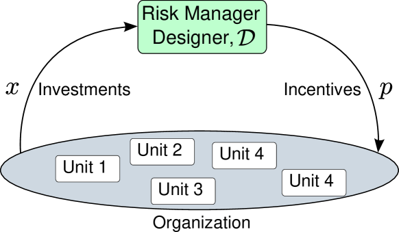
Figure 1: The interaction between the players (autonomous organizational units) of the underlying strategic game and the risk manager acting as mechanism designer, who observes players actions (investments) $x$ and provides additional incentives $p$.

The $N$-player strategic game, $\mathcal{G}$ is described as follows. Each player $i\in\mathcal{A}$ has a respective scalar decision variable $x_{i}$ such that

$$x=[x_{1},\ldots,x_{N}]\in\mathcal{X}\subset\mathbb{R}^{N},$$

where $\mathcal{X}$ is the convex, compact, and nonempty decision space of all players. The players make their decisions in accordance with their preferences modeled as customary by real valued utility functions

$$U_{i}(x):\mathcal{X}\rightarrow\mathbb{R}.$$

For analytical tractability, the player utility functions are chosen as continuous, differentiable, and strictly concave. It is important to note here that players do not reveal their utilities (preferences) to the designer. Application of a similar utility function approach to risk management has been discussed in detail in [14, Chap. 3], where the concave utilities are interpreted as “risk averse”.

While each player gains a utility from its decisions (investments), these resources also have a cost, which can be often expressed in monetary terms. We assume that that these costs are linear in the allocated resource, $\beta_{i}x_{i}$, where $\beta_{i}$ is the individual per unit cost factor. Each player $i$ aims to minimize its respective cost function

$$J_{i}(x)=\beta_{i}x_{i}-U_{i}(x)-p_{i}x_{i},$$ (1)

where the linear term $p_{i}x_{i}$ represents the incentive factor (or penalty if negative) provided to the player by the designer $\mathcal{D}$. Thus, player $i$ solves the optimization problem

$$\min_{x_{i}}J_{i}(x_{i},x_{-i}),$$

by choosing an appropriate $x_{i}$ given the decisions of all players denoted by $x_{-i}$ such that $x\in\mathcal{X}$. Formally, strategic game $\mathcal{G}$ is defined as:

Definition 1.

The strategic (noncooperative) game $\mathcal{G}$ is played among the set of selfish players, $\mathcal{A}$, of cardinality $N$, on the convex, compact, and non-empty decision space $\mathcal{X}\subset\mathbb{R}^{N}$, where

• $x=[x_{1},\ldots,x_{N}]\in\mathcal{X}$ denotes the actions of players

• $U_{i}(x):\mathcal{X}\rightarrow\mathbb{R}$ denotes the utility function of player $i\in\mathcal{A}$

• $J_{i}(x)=\beta_{i}x_{i}-U_{i}(x)-p_{i}x_{i}$ denotes the cost function of player $i\in\mathcal{A}$ for given parameters $b_{i}$ and $p_{i}$ $\forall i$,

such that each player $i$ solves its own optimization problem

$$\min_{x_{i}}J_{i}(x_{i},x_{-i}),$$

by choosing an appropriate $x_{i}$ given the decisions of all players denoted by $x_{-i}$.

The Nash equilibrium (NE) is a widely-accepted and useful solution concept in strategic games, where no player has an incentive to deviate from it while others play according to their NE strategies [31, 32]. The NE is at the same time the intersection point of players’ best responses obtained by solving their individual optimization problems. The NE of the game $\mathcal{G}$ in Definition 1 is formally defined as follows.

Definition 2.

The Nash equilibrium of the game $\mathcal{G}$ in Definition 1, is denoted by the vector $x^{*}=[x_{1}^{*},\ldots,x_{N}^{*}]\in\mathcal{X}$ and defined as

$$x_{i}^{*}:=\arg\min_{x_{i}}J_{i}(x_{i},x_{-i}^{*})\;\;\;\forall i\in\mathcal{A},$$

where $x_{-i}^{*}=[x_{1}^{*},\ldots,x_{i-1}^{*},x_{i+1}^{*},\ldots,x_{N}^{*}]$.

If some special convexity and compactness conditions are imposed to the game $\mathcal{G}$, then it admits a unique NE solution, which simplifies mechanism and algorithm design significantly. We refer to the Appendix A.1 as well as [33, 7, 1] for the details and an extensive analysis.

The risk manager (designer) $\mathcal{D}$ devises an incentive mechanism $\mathcal{M}$, which can be represented by the mapping $\mathcal{M}:\mathcal{X}\rightarrow\mathbb{R}^{N}$, and implemented through additional incentives (e.g. subsidies) in player cost functions, $p_{i}x_{i}$, above. Using incentive mechanism $\mathcal{M}$, the designer aims to achieve a certain risk management objective, which can be maximization of aggregate player utilities (expected aggregate benefit from risk-related investments) or an independent organizational target that depends on participation of all players such as deployment of a new risk management solution. These can be modeled using a designer objective function $V$ that quantifies the desirability of an outcome $x$ from the designers perspective. Formally, the function $V$ is defined as

$$V(x,U(x),p):\mathcal{X}\rightarrow\mathbb{R}.$$

Thus, the global optimization problem of the designer is

$$\max_{p}V(x,U_{i}(x),p),$$

which it solves by choosing the vector $p=[p_{1},\ldots,p_{N}]$, i.e. providing incentive factors to the players. Note that the designer objective $V$ (possibly) depends on player utilities $U=[U_{1},\ldots,U_{N}]$, yet the designer does not have direct knowledge on them. Furthermore, the risk manager may have only a limited budget $B$ to achieve its goal that leads to the additional constraint

$$\sum_{i=1}^{N}p_{i}x_{i}\leq B.$$

Mechanism design, as a field of game theory, studies designing the rules and structure of games such that their outcome achieve certain objectives [26, 23, 20, 11]. Two criteria a mechanism has to satisfy has already been described above. The player objective of minimizing own cost can also be called as preference-compatibility. Likewise, the designer objectives of maximizing $V$ or achieving a global goal can be interpreted as an efficiency criterion. The third criterion arises from the fact that the interaction between the designer and players of the game (Figure 1) may motivate the players to misrepresent their utilities to the designer. They can benefit from misrepresenting their utilities (exaggerating or diminishing the actual benefits of their investments) to receive higher incentives. Therefore, mechanism design has a third objective called interchangeably strategy-proofness, truth dominance, or incentive-compatibility in addition to the objectives of efficiency and preference-compatibility. All these three criteria are summarized in the following table:

Table 1: Three Criteria of Mechanism Design

Criterion	Formulation in the Model
Efficiency	Designer objective
Preference-	Players minimizing own costs
compatibility	(NE as operating point)
Strategy-Proofness	No player gains from cheating

2.1 Assumptions

Taking into account the breadth of the field mechanism design, it is useful to clarify the underlying assumptions of the model studied in this section. The environment where the players and designer interact is characterized by the following properties:

• The players and designer operate with limited resources, e.g. under budget and manpower constraints.

• The organizational structure imposes restrictions on available information to players and communication between them.

• The designer has no information on the preferences of individual players, but observes their actions and final costs.

The players share and compete for limited resources in the given environment under its information and communication constraints. The following assumptions are made on the designer and players:

• The designer is honest, i.e. does not try to deceive players.

• Each player acts alone and rationally according to own self interests.

• The players may try to deceive the designer by hiding or misrepresenting their own preferences.

• All players follow the rules of the mechanism imposed by the designer.

Implications of these assumptions and limitations of the presented model will be further discussed in Section 6.

3 Incentive Mechanism Design

This section presents two specific incentive mechanisms for risk management based on the model of the previous section. In the first mechanism, $\mathcal{M}_{1}$, the risk manager (designer) aims to maximize the aggregate benefit from security investments of units, which is the sum of player utilities. This objective is sometimes also called as “social welfare maximization”. The second mechanism, $\mathcal{M}_{2}$ represents a scenario in which the risk manager aims to align efforts of all units for deployment and operation of an organization-wide risk management solution. Both mechanisms (their iterative variants) satisfy the criteria in Table 1 under specific conditions. The interaction between the designer and players is visualized in Figure 2.

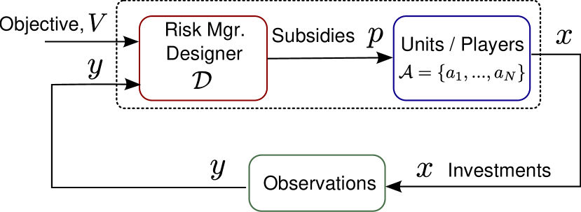
Figure 2: Interaction between risk manager (designer) and organizational units (players) as part of incentive mechanism design.

3.1 Welfare maximizing mechanism

The optimization problem $\min_{x_{i}}J_{i}(x)$ of player $i$ is a convex one and admits the unique solution

$$x_{i}^{*}=\left(\dfrac{\partial U_{i}(x)}{\partial x_{i}}\right)^{-1}(\beta_{i}-p_{i}),$$

under the strict concavity and continuous differentiability assumptions on $U_{i}$ [8]. Any such solution $x^{*}$ that solves all player optimization problems is by definition preference-compatible.

It is important to note that, if there was no incentive term, $p_{i}x_{i}$, in player cost, each unit would act according to self interest only resulting in a suboptimal result for the entire organization; a situation sometime termed as tragedy of commons. The designer can prevent this by providing a carefully selected incentive scheme [5, 4].

The risk manager $\mathcal{D}$ objective in mechanism $\mathcal{M}_{1}$ is to maximize sum of player utilities, $\sum_{i}U_{i}(x_{i})$. Considering that under the assumptions of Section 2 the risk manager does not know these utilities makes this goal paradoxical at first glance. However, the risk manager can actually achieve it in a carefully designed mechanism where it deduces the needed parameters for the solution from the observed actions of players.

Formally, the designer solves the constrained optimization problem

$$\max_{x}V(x)\Leftrightarrow\max_{x}\sum_{i}U_{i}(x)\text{ such that }\sum_{i}p_{i}x_{i}\leq B.$$ (2)

The optimal solution to this constrained problem by definition satisfies the efficiency criterion. The associated Lagrangian function is then

$$L(x)=\sum_{i}U_{i}(x)+\lambda\left(B-\sum_{i}p_{i}x_{i}\right),$$

where $\lambda\geq 0$ is a scalar Lagrange multiplier [8]. Under the concavity assumptions on $U_{i}$, this leads to

$$\dfrac{\partial L}{\partial x_{i}}=0\Rightarrow\dfrac{1}{p_{i}}\sum_{j=1}^{N}\dfrac{\partial U_{j}(x)}{\partial x_{i}}=\lambda,\;\forall i\in\mathcal{A},$$ (3)

and the associated budget constraint is

$$\dfrac{\partial L}{\partial\lambda}=0\Rightarrow\sum_{i}p_{i}x_{i}=B.$$ (4)

Meeting both the preference-compatibility and efficiency criteria requires alignment of player and designer optimization problems. This alignment can be achieved by choosing the Lagrange multiplier $\lambda$ and player incentive factors $p$ in such a way that

$$\dfrac{\beta_{i}-p_{i}}{p_{i}}+\dfrac{1}{p_{i}}\sum_{j\neq i}\dfrac{\partial U_{j}(x)}{\partial x_{i}}=\lambda,\;\forall i\in\mathcal{A},$$ (5)

and

$$\sum_{i}p_{i}\left(\dfrac{\partial U_{i}(x)}{\partial x_{i}}\right)^{-1}(\beta_{i}-p_{i})=B.$$ (6)

Any solution to the set of $N+1$ nonlinear equations (5)-(6) is by definition a Nash equilibrium as it lies at the intersection of the player best responses. These results are summarized in the following proposition.

Proposition 1.

Any solution of the mechanism $\mathcal{M}_{1}$ described above obtained from (5)-(6) is both player preference-compatible (based on the strategic game $\mathcal{G}$, given in Definition 1) and efficient, i.e. maximizes $\sum_{i}U_{i}(x)$.

If the designer $\mathcal{D}$ wants to compute the incentive factors $p$ directly by solving (5)-(6), it needs to ask each individual player $i$ for its utility, more specifically $\partial U_{i}(x)/\partial x_{j}$ $\forall j\in\mathcal{A}$. However, the players have now a motivation to misrepresent their utilities to the designer in order to gain a larger share of resources or incentive factors. To see this, consider a cheating player $i$ reporting $\tilde{U}_{i}$ to the designer instead of their true values. If the designer believes the player and solves (5)-(6) using these, then the resulting incentive factor $\tilde{p}$ will naturally be different from what it should have been, $p$. A selfish or malicious player can thus manipulate such a scheme, which by definition is not strategy-proof. Note that, the risk manager has access to costs $\beta_{i}x_{i}$ and actions $x_{i}$ of individual players, which can be, for example, part of an organizational reporting process.

One way to address the issue of strategy-proofness is to devise additional schemes to detect potential player misbehavior (for which players already have a motivation). This, however, brings an additional layer of overhead to the overall system both in terms of communication and computing requirements.

Alternatively, one can design an iterative mechanism that is based on observation of player actions $x$ instead of asking for their word (utilities). This approach is the basis of the iterative schemes that will be presented in Section 4.

3.2 Mechanism with global objective

The second mechanism, $\mathcal{M}_{2}$ differs from the social welfare maximizing one $\mathcal{M}_{1}$ discussed in the previous subsection. In this case, the designer has an organization-wide or “global” objective represented by the strictly concave and nondecreasing function $F(x)$ which does not directly depend on player utilities. This organization-wide objective could be, for example, deployment and operation of an organization-wide risk management solution that naturally requires cooperation from all units and an alignment of efforts.

In mechanism $\mathcal{M}_{2}$, the risk manager formally solves the constrained optimization problem

$$\max_{x}F(x)\text{ such that }\sum_{i}p_{i}x_{i}\leq B.$$ (7)

The associated Lagrangian function is then

$$L(x)=F(x)+\lambda\left(B-\sum_{i}p_{i}x_{i}\right),$$

where $\lambda>0$ is a scalar Lagrange multiplier. Note that the constraint is always active in this case due to the definition of $F(x)$. Under the concavity assumptions on $F(x)$, this leads to

$$\dfrac{\partial L}{\partial x_{i}}=0\Rightarrow\dfrac{1}{p_{i}}\dfrac{\partial F(x)}{\partial x_{i}}=\lambda,\;\forall i\in\mathcal{A},$$ (8)

and the associated budget constraint is

$$\dfrac{\partial L}{\partial\lambda}=0\Rightarrow\sum_{i}p_{i}x_{i}=B.$$ (9)

Combining this with the player optimization problems to ensure efficiency and preference-compatibility as in the previous subsection leads to

$$\dfrac{1}{p_{i}}\dfrac{\partial F(x)}{\partial x_{i}}=\lambda,\;\forall i\in\mathcal{A},$$ (10)

and

$$\sum_{i}p_{i}\left(\dfrac{\partial U_{i}(x)}{\partial x_{i}}\right)^{-1}(\beta_{i}-p_{i})=B,$$ (11)

which are direct counterparts of (5)-(6). As before, any solution constitutes a Nash equilibrium as it lies at the intersection of the player best responses.

Proposition 2.

Any solution of the mechanism $\mathcal{M}_{2}$ described above obtained from (10)-(11) is both player preference-compatible (based on the strategic game $\mathcal{G}$, given in Definition 1) and efficient, i.e. maximizes $F(x)$.

In mechanism $\mathcal{M}_{2}$, the risk manager has to evaluate the term $\partial F(x)/\partial x_{i}$ for each unit $i$, in addition to asking them for their utilities and cost factors. This term can be interpreted as the rate of contribution of each unit to the organization-wide objective. Since the risk manager sets this objective, it can be computed or estimated with reasonable accuracy. However, as before the solution of (10)-(11) also depends on individual unit utilities and cost factors. Therefore, mechanism $\mathcal{M}_{2}$ –similar to $\mathcal{M}_{1}$ – requires deployment of iterative methods in order to meet the criterion of strategy-proofness.

3.3 Interdependent Utilities and Linear Influence Model

In the presented model and analysis, utilities of individual players (units) may depend not only on their own actions but also on those of others, e.g. $U_{i}(x)=U_{i}([x_{1},\ldots,x_{N}])$. In other words, a unit benefits not only from own risk investments but also from efforts of other related units. Such utility functions are called interdependent or nonseparable in contrast to separable player utilities, $U_{i}(x_{i})$, that depend only own actions. If the player utilities are separable, then the player decisions are almost completely decoupled from each other except from external resource constraints (such as the incentives they receive from the designer). This simplifies development of decentralized schemes significantly.

One possible way of modeling interdependencies in player utilities is the linear influence model, which captures how actions (investments) of players (units) affect others. As a first-order approximation these effects are modeled as linear resulting in an influence matrix defined as

$$W:=\begin{cases}1&\text{, if }i=j,\\ w_{ij}&\text{, otherwise.}\end{cases}$$ (12)

where $0\leq w_{ij}\leq 1$ denotes the non-negative effect of unit $j$ (’s investment) on unit $i$. Notice that this effect may well be zero.

Define now the vector of effective investments $x^{e}=[x_{1}^{e},\ldots,x_{N}^{e}]$, where the effective investment of unit $i$ is

$$x^{e}_{i}:=\sum_{j}W_{ij}x_{j}=(Wx)_{i},$$

and $(\cdot)_{i}$ denotes the $i^{th}$ element of a vector.

Naturally, it is possible to develop more complex nonlinear models to capture interdependencies between units and their actions. However, given the limitations on information collection and accuracy, the linear first order approximation described provides a good starting point. Therefore, we will use linear influence model in the case of interdependent (non-separable) utilities for the rest of the paper.

Note that under the linear influence model, the nonseparable utility, $U_{i}(x)$, of player $i$ is given by

$$U_{i}(x^{e}_{i})=U_{i}\left((Wx)_{i}\right).$$

4 Iterative Incentive Mechanisms

Mechanisms $\mathcal{M}_{1}$ and $\mathcal{M}_{2}$ as defined in the previous section are shown to be efficient and preference-compatible (See Propositions 1 and 2) but not strategy-proof. This section presents two iterative variants of these mechanisms that satisfy all three criterion and can be implemented under information limitations.

4.1 Iterative mechanism with global objective

In the iterative mechanism with global objective, $\mathcal{IM}_{2}$, both the risk manager and units adopt an iterative scheme to facilitate information exchange that does not allow cheating, hence resulting in a strategy-proof mechanism. Specifically, the risk manager updates the Lagrangian multiplier $\lambda$ in (8) gradually according to

$$\lambda(n+1)=\lambda(n)+\kappa_{d}\left[\sum_{i}p_{i}(n)x_{i}(n)-B\right]^{+},$$ (13)

and computes the individual player incentive factors

$$p_{i}(n)=\dfrac{1}{\lambda(n)}\dfrac{\partial F(x(n))}{\partial x_{i}}.$$ (14)

Here, $n=1,\ldots$ denotes the iteration number or time-step. The units (players) in return react to given incentive factors by updating their investment decisions in order to minimize their own costs such that

$$\begin{array}[]{lll}x_{i}(n+1)&=&\phi x_{i}(n)\\ &+&(1-\phi)\left(\dfrac{\partial U_{i}(x(n))}{\partial x_{i}}\right)^{-1}(\beta_{i}-p_{i}(n))\;\;\forall i,\end{array}$$ (15)

where $0<\phi<1$ is a relaxation constant used by the players to prevent excessive fluctuations. Alternatively, this behavior can be justified with caution or inertia of the organizational units.

The equilibrium solution(s) of (13)-(15) clearly coincides with that of (10)-(11). Hence, the iterative mechanism $\mathcal{IM}_{2}$, assuming that it converges, solves the same problem as mechanism $\mathcal{M}_{2}$. Furthermore, it is strategy-proof since at each update step, the players make decisions according to their own self interests and do not have the opportunity of manipulating the system. To see this, assume otherwise and let player $i$ “misrepresent” its actions $\tilde{x}_{i}=x_{i}+\delta$ for some $\delta\in\mathbb{R}$. Then, the player’s instantaneous cost is $J_{i}(\tilde{x}_{i})>J_{i}(x_{i})$ at each step of the iteration. Hence, the players have no incentive to “cheat”. These results are summarized in the following theorem which extends Proposition 2:

Theorem 4.1.

Any solution of the iterative mechanism with global objective, $\mathcal{IM}_{2}$ described above and in Algorithm 1 is player preference-compatible, efficient, and strategy-proof.

Information flow and limitations play a crucial role in implementation of the iterative mechanism $\mathcal{IM}_{2}$. In practice, the risk manager is assumed to observe the actions of units which they have to reveal in order to receive incentives. Based on this information and the total budget, the risk manager can easily implement (13). Then, it only needs to estimate the individual marginal contributions of units to the overall objective, $\partial F(x(n))/\partial x_{i}$ at a given moment in order to decide on actual incentive factors in (14).

Likewise, given own cost estimates $\beta_{i}$ and incentive factor $p_{i}$, each unit (player) only has to determine the marginal benefit from its own actions, $\partial U_{i}(x(n))/\partial x_{i}$ in order to implement (15). If the unit has a separable utility, then this is simply equivalent to $\partial U_{i}(x_{i}(n))/\partial x_{i}$. In the interdependent utility case, under the linear influence model this quantity turns out to be the marginal benefit from the effective action,

$$\dfrac{\partial U_{i}(x(n))}{\partial x_{i}}=\dfrac{\partial U_{i}(x_{i}^{e}(n))}{\partial x_{i}^{e}}\dfrac{\sum_{j}W_{ij}x_{j}}{x_{i}}=\dfrac{\partial U_{i}(x_{i}^{e}(n))}{\partial x_{i}^{e}},$$

as a result of $W_{ii}=1$ and the definitions of respective quantities. Algorithm 1 summarizes the steps of the iterative mechanism with global objective, $\mathcal{IM}_{2}$.

Input: Designer: budget $B$ and global objective $F(x)$

Input: Players: cost factor $\beta_{i}$ and utilities $U_{i},\forall i$

Result: Player investments $x$ and incentive factors $p$

1

2Initial investments $x_{0}$ and incentive factors $p_{0}$ ;

3 repeat

4       begin Designer:

5             Observe player investments $x$ ;

6             Update $\lambda$ according to (13) ;

7             Estimate marginal contributions of players to global objective, $\partial F(x)/\partial x_{i}$ ;

8             foreach player $i$ do

9                   Compute incentive factor $p_{i}$ from (14) ;

10                  

11            end

12      end

13      begin Players:

14             foreach player $i$ do

15                   Estimate marginal utility $\partial U_{i}(x)/\partial x_{i}$ ;

16                   Compute investment $x_{i}$ from (15) ;

17                  

18            end

19      end

20until end of iteration (negotiation);

Algorithm 1 Iterative mechanism $\mathcal{IM}_{2}$

Convergence Analysis of $\mathcal{IM}_{2}$

A basic stability analysis is provided for a continuous-time approximation of the iterative mechanism with global objective, $\mathcal{IM}_{2}$. For tractability, let the player utilities be of the form $U_{i}=\alpha_{i}\log(x_{i})$. Further define the global objective function of the risk manager as $F(x):=\sum_{i}\gamma_{i}x_{i}$, for some $\gamma_{i}>0\;\forall i$.

Substituting $p_{i}$ with $\gamma_{i}/\lambda$, the continuous-time counterpart of (13)-(15) is

$$\dot{\lambda}=\dfrac{d\lambda}{dt}=\kappa_{\lambda}\dfrac{1}{\lambda}\left(\sum_{i}\gamma_{i}x_{i}(n)-B\right)$$ (16)

$$\dot{x}_{i}=-\kappa_{i}\dfrac{\partial J_{i}}{\partial x_{i}}=\kappa_{i}\left(\dfrac{\alpha_{i}}{x_{i}}+\dfrac{\gamma_{i}}{\lambda}-\beta_{i}\right)\;\;,\forall i\in\mathcal{A}.$$

where $t$ denotes time and $\kappa_{\lambda},\;\kappa_{i}>0$ are step-size constants. As in the discrete-time version, the players adopt here a gradient best response algorithm. Define the Lyapunov function

$$V_{L}:=\frac{1}{2}\left(\dfrac{\sum_{i}\gamma_{i}x_{i}-B}{\lambda}\right)^{2}+\frac{1}{2}\sum_{i}\left(\dfrac{\alpha_{i}}{x_{i}}+\dfrac{\gamma_{i}}{\lambda}-\beta_{i}\right)^{2},$$

which is nonnegative except at the solution(s) of (13)-(15), i.e. $V_{L}(x^{*},\lambda^{*})=0$.

Taking the derivative of $V_{L}$ with respect to time yields

$$\dot{V}_{L}(x,\lambda)=-2\dfrac{\sum_{i}\gamma_{i}x_{i}}{\lambda^{3}}\left(\dfrac{\sum_{i}\gamma_{i}x_{i}-B}{\lambda}\right)^{2}-\sum_{i}\dfrac{\alpha_{i}}{x_{i}^{2}}\left(\dfrac{\alpha_{i}}{x_{i}}+\dfrac{\gamma_{i}}{\lambda}-\beta_{i}\right)^{2}.$$

Consider the region where $F(x)=\sum_{i}\gamma_{i}x_{i}>0$. Then, there exists an $\epsilon>0$ such that

$$\dot{V}_{L}(x,\lambda)\leq\epsilon V_{L}<0,\;\;\forall(x,\lambda)\neq(x^{*},\lambda^{*}),$$

i.e. for any point of the trajectory $(x,\lambda)$ not equal to a solution of (13) and (15). Thus, the continuous-time algorithm is exponentially stable [22] on the set $\mathcal{\bar{X}}:=\{x\in\mathcal{X}:F(x)>0\}$. This result, which is summarized in the next theorem, is a strong indicator of fast convergence [9] of the discrete-time iterative pricing mechanism (14)-(17).

Proposition 3.

The continuous-time approximation of the iterative mechanism $\mathcal{IM}_{2}$, given by (16) exponentially converges to a solution of (13)-(15) on the set $\mathcal{\bar{X}}=\{x\in\mathcal{X}:F(x)>0\}$.

The exponential convergence result above indicates a very fast convergence rate. To see this, let $x(0)$ be the initial player investments and $x^{*}$ denote a solution of (13)-(15). Then, for the player investments $x(t)$ under continuous-time approximation of the iterative mechanism $\mathcal{IM}_{2}$ the following holds:

$$\left\|x(t)-x^{*}\right\|\leq\alpha\left\|x(0)-x^{*}\right\|e^{-\beta t},$$

for $t\geq 0$ and some $\alpha,\beta>0$. In other words, the investment levels approach their equilibrium values exponentially fast.

4.2 Iterative welfare maximizing mechanism

The iterative welfare maximizing mechanism $\mathcal{IM}_{1}$ extends mechanism $\mathcal{M}_{1}$. Same as the previous mechanism, the risk manager updates the Lagrangian multiplier $\lambda$ according to (13) and the unit updates are given by (15).

However, the computation of individual player incentive factors is more involved due to the dependence of the objective (welfare maximization) on individual player utilities

$$p_{i}(n)=\dfrac{1}{\lambda(n)}\sum_{j}\dfrac{\partial U_{j}(x(n))}{\partial x_{i}},$$ (17)

which follows from (5). At first glance, it seems that the designer has to ask players again for their marginal utility which defeats the purpose of the iterative approach, namely ensuring strategy-proofness. Fortunately, the designer can circumvent this issue by utilizing side information, in this case player cost factors $\beta$, within the linear influence model.

It directly follows from the linear influence model that

$$\dfrac{\partial U_{j}}{\partial x_{i}}=\dfrac{\partial U_{j}}{\partial x_{j}^{e}}\dfrac{\partial x_{j}^{e}}{\partial x_{i}}=\dfrac{\partial U_{j}}{\partial x_{j}^{e}}W_{ji}=\dfrac{\partial U_{j}}{\partial x_{j}}W_{ji}.$$

The actions of any player $i$ chosen according to a (relaxed) best response (15), and observed by the designer yields the information

$$\dfrac{\partial U_{i}(x)}{\partial x_{i}}=\beta_{i}-p_{i}$$

to the designer. Hence, the substitution

$$\sum_{j}\dfrac{\partial U_{j}(x(n))}{\partial x_{i}}=\sum_{j}(\beta_{i}-p_{i})W_{ji},\;\forall i,j\,,$$

can be used in (17) to obtain

$$\lambda p=W^{T}(\beta-p).$$

Thus, the designer implements

$$p=(W^{T}+\lambda I)^{-1}W^{T}\beta$$ (18)

together with (13) to determine player incentive factors. Here, $(\cdot)^{T}$ denotes the transpose operator and $I$ the identity matrix. These results are summarized in the following theorem which extends Proposition 1:

Theorem 4.2.

Any solution of the iterative mechanism with global objective, $\mathcal{IM}_{1}$ described above and in Algorithm 2 is player preference-compatible, efficient, and strategy-proof.

The information structure in mechanism $\mathcal{IM}_{1}$ is similar to that of $\mathcal{IM}_{2}$ with the following differences. In $\mathcal{IM}_{1}$, the risk manager has to estimate the linear dependencies in the system represented by the matrix $W$ and observe cost factors $\beta$ of units in addition to their investments. These information requirements are due to the complex nature of the welfare maximization objective, which necessitates additional (indirect) communication between the risk manager and units in practice. Algorithm 2 summarizes the steps of the welfare maximizing mechanism $\mathcal{IM}_{1}$.

Input: Designer: budget $B$ and objective $\sum_{i}U_{i}$

Input: Players: cost factor $\beta_{i}$ and utilities $U_{i},\forall i$

Result: Player investments $x$ and incentive factors $p$

1

2Initial investments $x_{0}$ and incentive factors $p_{0}$ ;

3 repeat

4       begin Designer:

5             Observe player actions $x$ and cost factors $\beta$ ;

6             Estimate the linear influence matrix $W$ ;

7             Update $\lambda$ according to (13) ;

8             Compute incentive factors $p$ from (18) ;

9            

10      end

11      begin Players:

12             foreach player $i$ do

13                   Estimate marginal utility $\partial U_{i}(x)/\partial x_{i}$ ;

14                   Compute investment $x_{i}$ from (15) ;

15                  

16            end

17      end

18until end of iteration (negotiation);

Algorithm 2 Iterative mechanism $\mathcal{IM}_{1}$

Convergence Analysis of $\mathcal{IM}_{1}$

A basic stability analysis is provided for a continuous-time approximation of the iterative mechanism $\mathcal{IM}_{1}$ similar to the one of the $\mathcal{IM}_{2}$ in the previous subsection. For tractability, let the player utilities be of the form $U_{i}=\alpha_{i}\log(x_{i})$ as before.

Substituting $p_{i}$ with

$$p_{i}=\dfrac{\beta_{i}}{1+\lambda},$$

which follows from (18) and $W=I$, the continuous-time counterpart of (13) and (15) is

$$\dot{\lambda}=\dfrac{d\lambda}{dt}=\kappa_{\lambda}\dfrac{1}{1+\lambda}\left(\sum_{i}\beta_{i}x_{i}(n)-B\right)$$ (19)

$$\dot{x}_{i}=-\kappa_{i}\dfrac{\partial J_{i}}{\partial x_{i}}=\kappa_{i}\left(\dfrac{\alpha_{i}}{x_{i}}+\dfrac{\beta_{i}}{1+\lambda}-\beta_{i}\right)\;\;,\forall i\in\mathcal{A}.$$

where $t$ denotes time and $\kappa_{\lambda},\;\kappa_{i}>0$ are step-size constants. As in the discrete-time version, the players adopt here a gradient best response algorithm. Define the Lyapunov function

$$\bar{V}_{L}:=\frac{1}{2}\left(\dfrac{\sum_{i}\beta_{i}x_{i}-B}{1+\lambda}\right)^{2}+\frac{1}{2}\sum_{i}\left(\dfrac{\alpha_{i}}{x_{i}}+\dfrac{\beta_{i}}{1+\lambda}-\beta_{i}\right)^{2},$$

which is nonnegative except at the solution(s) of (13) and (15), i.e. $\bar{V}_{L}(x^{*},\lambda^{*})=0$.

Taking the derivative of $\bar{V}_{L}$ with respect to time yields

$$\dot{\bar{V}}_{L}(x,\lambda)=-2\dfrac{\sum_{i}\beta_{i}x_{i}}{(1+\lambda)^{3}}\left(\dfrac{\sum_{i}\beta_{i}x_{i}-B}{1+\lambda}\right)^{2}-\sum_{i}\dfrac{\alpha_{i}}{x_{i}^{2}}\left(\dfrac{\alpha_{i}}{x_{i}}+\dfrac{\beta_{i}}{1+\lambda}-\beta_{i}\right)^{2}.$$

Consider the region where $\sum_{i}\beta_{i}x_{i}>0$. Then, there exists an $\epsilon>0$ such that

$$\dot{\bar{V}}_{L}(x,\lambda)\leq\epsilon\bar{V}_{L}<0,\;\;\forall(x,\lambda)\neq(x^{*},\lambda^{*}),$$

i.e. for any point of the trajectory $(x,\lambda)$ not equal to a solution of (13) and (15). Thus, the continuous-time algorithm is exponentially stable [22] on the set $\mathcal{\tilde{X}}:=\{x\in\mathcal{X}:\sum_{i}\beta_{i}x_{i}>0\}$. This result, which is summarized in the next theorem, is a strong indicator of fast convergence [9] of the discrete-time iterative pricing mechanism $\mathcal{IM}_{1}$.

Proposition 4.

The continuous-time approximation of the iterative mechanism $\mathcal{IM}_{1}$, given by (19) exponentially converges to a solution on the set $\mathcal{\tilde{X}}:=\{x\in\mathcal{X}:\sum_{i}\beta_{i}x_{i}>0\}$.

5 Use Case Scenario and Numerical Analysis

In order to illustrate the incentive mechanism framework for risk management, a use case scenario is described next. Since most organizations do not openly publish their actual risk management structure or numbers, this scenario is naturally hypothetical and the numbers in the subsequent numerical analysis do not necessarily coincide with real world counterparts.

5.1 Example Use Case Scenario

In this subsection, a possible use cases scenario is described for a large-scale enterprise with multiple autonomous business units, denoted by set $\mathcal{A}$, who collaborate and share IT infrastructure in order to provide various services and products. In addition to the business units, the enterprise headquarters has a special security risk management division, which will be simply referred to as “risk manager” here. The task of the risk manager, $\mathcal{D}$, is successful deployment and operation of security and IT risk management projects that entail enterprise-wide computer-assisted information collection (observation), risk assessment (decision making), and mitigation (control).

The results and algorithms described in this paper can be utilized to develop a manual risk management strategy as well as a technical system to handle a large number of business units and multiple concurrent risk management projects. For simplicity and as a special case of the latter, this scenario focuses on the former.

Let the risk manager start a project to improve robustness of the IT systems involved in a product against security threats. The success of the project naturally depends on collaboration of the $6$ specific business units involved at various stages of the product in question. However, not each unit plays an equal role in creation of the product, and hence, their risk exposure is different. Therefore, those units with a more significant role have to make a larger investment to the project and their IT systems.

During the project, the divisions have to provide accurate information on their business and networked systems. At the operational phase, each division allocates manpower and resources for the proper operation of the system. Hence, participation in this risk management project is associated with a certain cost to each unit in terms of investments and manpower. Although each unit sees a certain amount of value in the new risk management system, if they are left alone to themselves, their contributions may not be sufficient for the successful realization of the risk management system. Thus, the risk manager uses parts of its budget for subsidizing individual unit investments, if necessary in the form of manpower and expertise.

Let $x=[x_{1},x_{2},\ldots,x_{6}]$ denote the investments (project contributions) of business units. Their contribution to the project is evaluated using the multi-variable objective function $F(x)$, which describes the goal of the entire project. The individual marginal contribution of a business unit $i$ (one of six) to the project goal at a given (project) state is given by the derivative, $\partial F(x)/\partial x_{i}$. It is important to note that risk manager may not know the exact form of $F(x)$ before hand, and has to estimate $\partial F(x)/\partial x_{i}$ for each business unit $i$ at a given state.

The goal of the risk manager is to ensure the success of the project, which may be captured by making the objective function achieve a certain minimum threshold value, i.e. $F(x)>V_{threshold}$. The subsidies given to the units (monetarily or in the form of assistance) are determined in proportion to their current investments. For example, the business unit $i$ receives $p_{i}x_{i}$. These subsidies have to be of course within the allocated budget, i.e. $\sum_{i=1}^{6}p_{i}x_{i}\leq B$. Note that, the budget in question is periodic, e.g. $B$ units per month or year.

The interaction between the risk manager and individual units is designed according to Algorithm 1 based on the $\mathcal{IM}_{2}$. The actual time-scale of the iteration depends on the specific requirements of the enterprise. For example, the risk managers and representatives from the units may come together in weekly or bi-weekly intervals to evaluate the progress, which gives some time to the units and manager for updating own evaluations on marginal benefits and contributions, respectively. We next present a numerical example to further illustrate the scenario described.

5.2 Numerical Analysis

Based on the use case scenario, an example is numerically analyzed with a risk manager and $6$ units, who implement the iterative mechanism $\mathcal{IM}_{2}$ using Algorithm 1. The budget is $B=3$, the global objective function of the risk manager is $F(x)=\sum_{i=1}^{6}\gamma_{i}x_{i}$, where $\gamma=[0.8,\;0.4,\;0.5,\;0.2,\;0.3,\;0.1]$, the utilities of units are in the form of $U_{i}(x_{i})=\alpha_{i}\log(x_{i})$, where $\alpha=[0.9,\;0.7,\;0.6,\;0.8,\;0.2,\;0.4]$, and the unit cost factor is $\beta=3$ for all six units. Each unit starts the iteration with an initial investment of $x_{i}=0.5\;\forall i$ and receives an initial incentive factor of $p_{i}=0.3\;\forall i$. The measurement units of the budget $B$ and investments $x$ are assumed to be on the order of millions of dollars. The step-size constants are chosen as $\kappa_{d}=0.05$ and $\phi=0.3$. The success of the project is decided by whether the objective function passes minimum threshold of $2.5$, i.e. $F(x^{*})>2.5$.

The evolution of unit investment levels $x(n)$ is shown in Figure 3 and the associated incentive factors $p(n)$ in Figure 4. The first unit, which contributes the most to the objective receives a higher amount of aid from the risk manager than others. The algorithm converges fast, in $10-15$ steps, for the given parameters, as indicated by the exponential convergence of its continuous-time counterpart. For a time interval of $1-2$ weeks per iteration, this corresponds to $3-6$ months in practice. Although this convergence time may seem as a disadvantage at the first glance, in a practical project with highly varying parameters, such an online algorithm may even be beneficial in terms of adaptability over time.

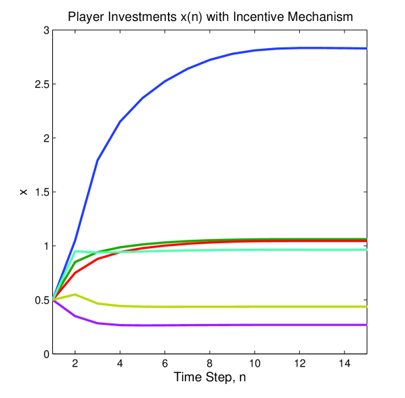
Figure 3: The evolution of unit investment levels $x(n)$ under Algorithm 1.

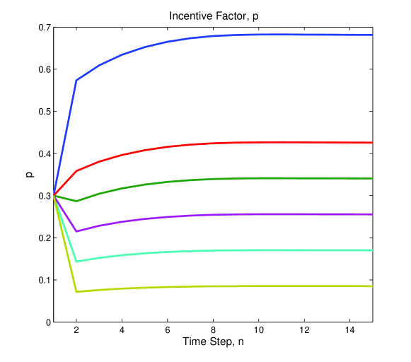
Figure 4: The evolution of incentive factors $p(n)$ under Algorithm 1.

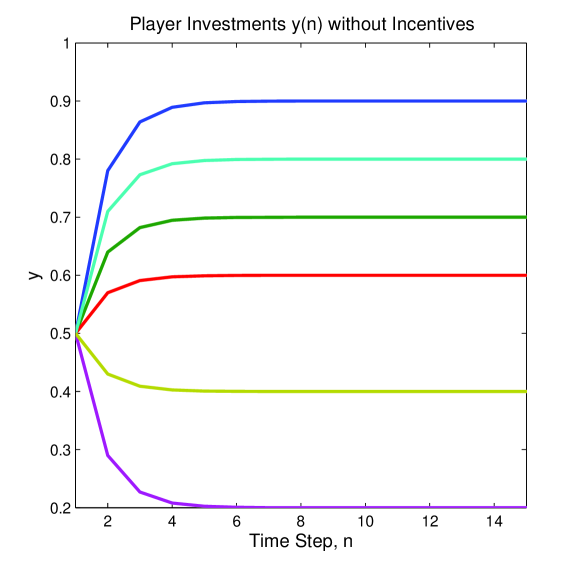
Figure 5: The evolution of unit investment levels $y(n)$ without any incentive mechanism implemented.

In contrast, the investment results of units without any incentive mechanism in place, $y(n)$, is shown in Figure 5. A comparison of the objective function $F(x)$ with and without an incentive mechanism is depicted in Figure 6. Naturally, this improvement comes at an expense of the budget $B$ spent entirely by the risk manager.

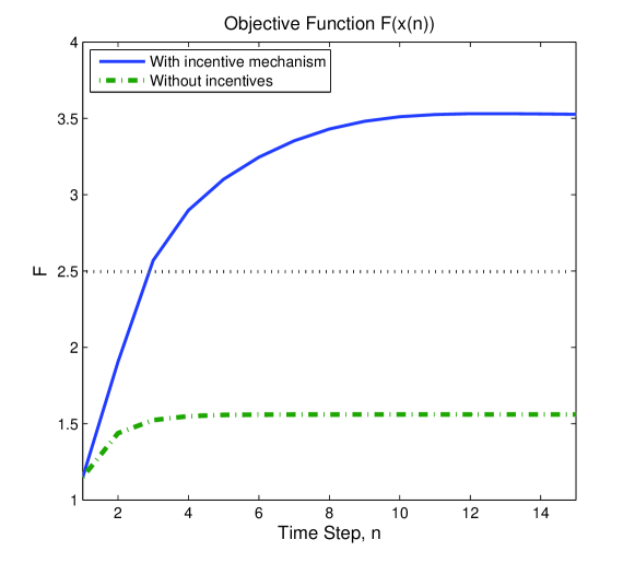
Figure 6: A comparison of the objective function $F(x(n))$ with and without an incentive mechanism. Under the incentive mechanism it passes the success threshold of $2.5$.

6 Literature Review

Building upon its successful applications to economics and engineering (e.g. networks), game theory has been recently utilized to model and analyze security problems [2]. Similar formalization efforts have been ongoing in the risk management area with the goal of developing analytical approaches to (security) risk analysis, management, and associated decision making [14, 3, 17, 30]. Unsurprisingly, game theory enjoys an increased interest in the risk management community [24, 21, 6, 16], as it provides a valuable and relevant mathematical framework [2, 7, 13]. Recently, a game theoretic approach has been developed for security and risk-related decision making and investments in [28, 27].

Mechanism design [26, 23, 20] is a field of game theory, where a designer imposes rules on the underlying strategic (noncooperative) game in order to achieve certain desirable objectives such as social welfare maximization or a system-wide goal. Hence, mechanism design can be viewed as a reverse engineering of games. It is especially useful in developing analytical frameworks for incentive mechanisms. Recently, there has been widespread interest in using mechanism design for modeling, analyzing and solving problems in network resource allocation problems that are decentralized in nature [20, 38, 23, 25, 37, 18]. It has also been applied to resource allocation in the context of engineering optimization [15]. A basic game design approach to security investments in the risk management context has been discussed in [2].

The presented incentive mechanism framework makes use of both mechanism design [26, 23, 20, 11] and game theory [7, 13], which provide solid analytical and conceptual foundations. In contrast to many existing studies [10, 19, 12] focusing on answering the question of “which mechanisms are possible to design”, this work adopts a constructive approach to develop a practical methodology and applies it to security risk management. Despite sharing the game-theoretic approach of earlier work [28, 27], it distinguishes from these through the mechanism design framework developed on top of the game. A similar perspective has been briefly discussed in [2, Chap. 6], which however has not taken into account incentive-compatibility aspects.

The article [15], which shares a similar goal as this one, discusses the problem of designing an allocation scheme that leads to truthful reporting by the engineers and allocation of the scarce resources within the VCG framework. This work distinguishes from [15] in multiple ways in addition to its focus on risk management. First, the mechanisms discussed here are iterative, enable operation even under limited information, and do not require any direct revelation of preferences by the users or risk manager. Similar iterative schemes have been analyzed in depth in the networking literature, e.g. see [38, 36, 1]. Second, the sufficient conditions for convergence and operation of the iterative mechanisms here are not as restrictive as in [15]. Finally, the properties of iterative interaction algorithms are analyzed rigorously from a dynamical system perspective and their rapid convergence is proven.

7 Discussion and Conclusion

The analytical incentive mechanism design framework presented can not only be used to derive guidelines for handling incentives in risk management but also to develop computer-assisted schemes. The abstract nature of the framework is an advantage in terms of widespread applicability to diverse situations and organization types. In order to satisfy all three objectives of efficiency, preference-compatibility and strategy-proofness, iterative incentive mechanisms and related algorithms are developed which also allow implementation under information limitations. These mechanisms are very straightforward to analyze and implement numerically, which is especially useful since any practical implementation of such incentive mechanism will most probably involve some kind of computer-assistance. The risk manager has then the option to evaluate various scenarios through simulations before actual deployment. This is illustrated with a hypothetical deployment scenario and a numerical example.

The presented inventive mechanism framework can be extended in multiple directions. One immediate extension is multiple decision variables. For example, units may need to distinguish between monetary investments and local resources such as manpower. Similarly, the risk manager may utilize multiple separate incentive factors. A related but more challenging extension is multi-criteria decision making, where preferences are not simply expressed through scalar valued functions such as $U$ and $F$. This is an open research area also in decision and optimization theories.

The limitations of the utility-based approach adopted here is also worth noting. The expression of preferences through specific (continuous, differentiable) functions is obviously a simplification to facilitate devising analytically tractable models. However, as it can be seen in Sections 4 and 5, the resulting algorithms do not necessarily require the players estimate their whole utility beforehand. A step-by-step iterative estimation process is fully sufficient to establish and communicate these preferences.

An underlying assumption of the model until now has been the fixed nature of player preferences or utility functions. Under this assumption, the risk manager can influence unit decisions only by introducing additive incentive factors to their cost structure as discussed. In reality however, the unit preferences are open to changes through psychological factors. The arts of persuasion and politics may “shift” the utility curves in the model. Quantification of such factors is obviously a significant yet open research challenge.

An approach closely related to the strategic (noncooperative) game framework discussed in this paper, is based on coalitional (cooperative) games [13, 35]. How to motivate team building and cooperation in security and risk management has been recently discussed in [34] as well as in[2, Chap. 6]. This alternative approach provides a complementary and potentially very interesting research direction.

Some of the other open research directions follow directly from relaxing the assumptions in Section 2. Improving the robustness of the incentive mechanisms against malicious units who do not follow the rules or have utilities orthogonal to other users (sometimes referred to as adversarial mechanism design) is an emerging and relevant research area. Detection of such misbehavior is also of both practical and theoretical interest. In parallel to users, the relaxation of the assumption on risk manager’s honesty leads to similarly interesting questions such as how can a unit detect and respond to misbehavior (e.g. unfairness) of the risk manager.

Appendix

Existence and Uniqueness of Nash Equilibrium

This appendix revisits the analysis in [1, 33] on existence and uniqueness of Nash equilibrium.

In the strategic game $\mathcal{G}$ given in Definition 1, the strategy (decision) space of the players is assumed to be convex, compact, and has a nonempty interior. Furthermore, the cost functions of the players, $J_{i},\;\;i\in\mathcal{A}$, is strictly convex in $x_{i}$ and at least twice continuously differentiable due to its definition as well as those of utility functions $U_{i},\;\;i\in\mathcal{A}$. Therefore, the game $\mathcal{G}$ admits (at least) a Nash equilibrium from Theorem 4.4 in [7, p.176].

Next, additional conditions are imposed such that the game $\mathcal{G}$ admits a unique NE solution. Toward this end, define the pseudo-gradient operator

$$\overline{\nabla}J:=\left[\partial J_{1}(x)/\partial x_{1}\cdots\partial J_{N}(x)/\partial x_{N}\right]^{T}:=g(x).$$ (20)

Subsequently, let the $N\times N$ matrix $G(x)$ be the Jacobian of $g(x)$ with respect to $x$:

$$G(x):=\begin{pmatrix}b_{1}&a_{12}&\cdots&a_{1N}\\ \vdots&&\ddots&\vdots\\ a_{N1}&a_{N2}&\cdots&b_{N}\ \end{pmatrix}\;,$$ (21)

where $b_{i}$ and $a_{ij}$ are defined as $b_{i}:=\frac{\partial^{2}J_{i}(x)}{\partial x_{i}^{2}}$ and $a_{i,j}:=\frac{\partial^{2}J_{i}(x)}{\partial x_{i}\partial x_{j}}$, respectively.

Assumption 1.

The symmetric matrix $G(x)+G(x)^{T}$, where $G(x)$ is defined in (21), is positive definite, i.e. $G(x)+G(x)^{T}>0$ for all $x\in\mathcal{X}$.

Assumption 2.

The strategy space $\mathcal{X}$ of the game $\mathcal{G}$ can be described as

$$\mathcal{X}:=\{x\in\mathbb{R}^{N}\,:\,h_{j}(x)\leq 0,\;j=1,\,2,\,\ldots r\},$$ (22)

where $h_{j}:\mathbb{R}^{N}\rightarrow\mathbb{R},j=1,\,2,\,\ldots r$, $h_{j}(x)$ is convex in its arguments for all $j$, and the set $\mathcal{X}$ is bounded and has a nonempty interior. In addition, the derivative of at least one of the constraints with respect to $x_{i}$, $\{dh_{j}(x)/dx_{i},\;j=1,\,2,\,\ldots r\}$, is nonzero for $i=1,\,2,\,\ldots N$, $\forall x\in\mathcal{X}$.

Now, revisiting the analysis in [1, 33], it is shown that the game $\mathcal{G}$ admits a unique Nash equilibrium under Assumptions 1 and 2.

In view of Assumption 2, the Lagrangian function for player $i$ in this game is given by

$$L_{i}(x,\mu)=J_{i}(x)+\sum_{j=1}^{r}\mu_{i,j}h_{j}(x),$$ (23)

where $\mu_{i,j}\geq 0,\;j=1,\,2,\,\ldots r$ are the Lagrange multipliers of player $i$ [8, p. 278]. We now provide a proposition for the game $\mathcal{G}$ with conditions similar to the well known Karush-Kuhn-Tucker necessary conditions (Proposition 3.3.1, p. 310, [8]).

Proposition 5.

Let $x^{*}$ be a NE point of the game $\mathcal{G}$ and Assumptions 1-2 hold. There exists then a unique set of Lagrange multipliers, $\{\phi_{i,j}:\;j=1,\,2,\,\ldots r,\;i=1,\,2,\,\ldots N\}$, such that

$$\begin{array}[]{r}\dfrac{dL(x^{*},\phi)}{dx_{i}}=\dfrac{dJ_{i}(x^{*})}{dx_{i}}+\displaystyle{\sum_{j=1}^{r}\phi_{i,j}^{*}\dfrac{dh_{j}(x^{*})}{dx_{i}}}=0,\\ i=1,\,2,\,\ldots N,\\ \phi_{i,j}\geq 0,\;\;\forall i,j,\text{ and }\;\phi_{i,j}=0,\;\;\forall j\notin A_{i}(\mathbf{x}^{*}),\forall i\,,\end{array}$$

where $A_{i}(x^{*})$ is the set of active constraints in $i^{th}$ player’s minimization problem at NE point $x^{*}$.

Proof.

The proof essentially follows lines similar to the ones of the Proposition 3.3.1 of [8], where the penalty approach is used to approximate the original constrained problem by an unconstrained problem that involves a violation of the constraints. The main difference here is the repetition of this process for each individual $x_{i}$ at the NE point $x^{*}$. ∎

Define now a more compact notation the vector of Lagrangian functions as $L:=[L_{1},\ldots,L_{N}]$, and the $N\times N$ diagonal matrix of Lagrange multipliers for the $j^{th}$ constraint as $\Phi_{j}=\rm{diag}[\phi_{1,j},\phi_{2,j},\ldots\phi_{N,j}]$.

By Proposition 5 and Assumption 2, a NE point $x^{(1)}$ satisfies

$$\overline{\nabla}L(x^{(1)},\Phi^{(1)})=g(x^{(1)})+\sum_{j=1}^{r}\Phi_{j}^{(1)}\overline{\nabla}h_{j}(x^{(1)})=0,$$ (24)

where $\Phi_{j}^{(1)}\geq 0$ is unique for each $j$. Assume there are two different NE points $x^{(0)}$ and $x^{(1)}$. Then, one can also write the counterpart of (24) for $x^{(0)}$. Following an argument similar to the one in the proof of Theorem 2 in [33], one can show that this leads to a contradiction. We present a brief outline of a simplified version of that proof for the sake of completeness.

Multiplying (24) and its counterpart for $x^{(0)}$ from left by $(x^{(0)}-x^{(1)})^{T}$, and then adding them together, we obtain

$$\begin{array}[]{rcl}0&=&(x^{(0)}-x^{(1)})^{T}\overline{\nabla}L(x^{(1)},\Phi^{(1)})\\ &&+\left(\overline{\nabla}L(x^{(1)},\Phi^{(1)})\right)^{T}(x^{(0)}-x^{(1)})\\ &&+(x^{(1)}-x^{(0)})^{T}\overline{\nabla}L(x^{(0)},\Phi^{(0)})\\ \\ &=&(x^{(0)}-x^{(1)})^{T}\left(g(x^{(1)})-g(x^{(0)})\right)\\ &&+\left(g(x^{(1)})-g(x^{(0)})\right)^{T}(x^{(0)}-x^{(1)})\\ &&+(x^{(1)}-x^{(0)})^{T}\sum_{j=1}^{r}[\Phi_{j}^{(1)}\overline{\nabla}h_{j}(x^{(1)})\\ &&-\Phi_{j}^{(0)}\overline{\nabla}h_{j}(x^{(0)})].\\ \end{array}$$ (25)

Define the strategy vector $x(\theta)$ as a convex combination of the two equilibrium points $x^{(0)}\,,\,x^{(1)}$ :

$$x(\theta)=\theta x^{(1)}+(1-\theta)x^{(0)},$$

where $0<\theta<1$. Take the derivative of $g(x(\theta))$ with respect to $\theta$,

$$\dfrac{dg(x(\theta))}{d\theta}=G(x(\theta))\frac{dx(\theta)}{d\theta}=G(x(\theta))(x^{(1)}-x^{(0)}),$$ (26)

where $G(x)$ is defined in (21). Integrating (26) over $\theta$ yields

$$g(x^{(1)})-g(x^{(0)})=\left[\int_{0}^{1}G(x(\theta))d\theta\right](x^{(1)}-x^{(0)}).$$ (27)

Multiplying (27) from left by $(x^{(1)}-x^{(0)})^{T}$, the transpose of (27) from right by $(x^{(1)}-x^{(0)})$, and adding these two terms yields

$$(x^{(1)}-x^{(0)})^{T}\left[\int_{0}^{1}G(x(\theta))+G^{T}(x(\theta))d\theta\right](x^{(1)}-x^{(0)}).$$ (28)

Since $G(x(\theta))+G^{T}(x(\theta))$ is positive definite by Assumption 1 and the sum of two positive definite matrices is positive definite, the matrix $\bar{G}:=\int_{0}^{1}G(x(\theta))+G^{T}(x(\theta))d\theta$ is positive definite.

Similarly, we have

$$\dfrac{d\overline{\nabla}h(x(\theta))}{d\theta}=H(x(\theta))\frac{dx(\theta)}{d\theta}=H(x(\theta))(x^{1}-x^{0}),$$ (29)

where $H(x)$ is the Jacobian of $\overline{\nabla}h(x)$ and positive definite due to convexity of $h(x)$ by definition. The third term in (25)

$$\begin{array}[]{r}(x^{(0)}-x^{(1)})^{T}\sum_{j=1}^{r}[\Phi_{j}^{(0)}\overline{\nabla}h_{j}(x^{(0)})-\Phi_{j}^{(1)}\overline{\nabla}h_{j}(x^{(1)})],\end{array}$$

is less than

$$\sum_{j=1}^{r}[\Phi_{j}^{(1)}-\Phi_{j}^{(0)}][h_{j}(x^{(1)})-h_{j}(x^{(0)})],$$

due to convexity of $h(x)$. Since for each constraint $j$, $h_{j}(x)\leq 0\;\forall x$, $\Phi_{j}^{(i)}h_{j}(x^{(i)})=0,\;i=0,1$, and $\Phi_{j}$ is positive definite, where the latter two follow from Karush-Kuhn-Tucker conditions, this term is also non-positive.

The sum of the first two terms in (25) are the negative of (28), which is strictly positive for all $x^{(1)}\neq x^{(0)}$. Hence, (25) is strictly negative which leads to a contradiction unless $x^{(1)}=x^{(0)}$. Thus, there exists a unique NE point in the game $\mathcal{G}$.

References

- [1] Alpcan, T.: Noncooperative games for control of networked systems. Ph.D. thesis, University of Illinois at Urbana-Champaign, Urbana, IL (2006)
- [2] Alpcan, T., Başar, T.: Network Security: A Decision and Game Theoretic Approach. Cambridge University Press (2011). URL http://www.tansu.alpcan.org/book.php
- [3] Alpcan, T., Bambos, N.: Modeling dependencies in security risk management. In: Proc. of 4th Intl. Conf. on Risks and Security of Internet and Systems (Crisis). Toulouse, France (2009)
- [4] Alpcan, T., Pavel, L.: Nash equilibrium design and optimization. In: Proc. of Intl. Conf. on Game Theory for Networks (GameNets 2009). Istanbul, Turkey (2009)
- [5] Alpcan, T., Pavel, L., Stefanovic, N.: A control theoretic approach to noncooperative game design. In: Proc. of 48th IEEE Conf. on Decision and Control. Shanghai, China (2009)
- [6] and, E.P.C.: Risks and games: Intelligent actors and fallible systems. In: Proc. of 2nd Intl. Symp. on Engineering Systems. Cambridge, MA, USA (2009)
- [7] Başar, T., Olsder, G.J.: Dynamic Noncooperative Game Theory, 2nd edn. Philadelphia, PA: SIAM (1999)
- [8] Bertsekas, D.: Nonlinear Programming, 2nd edn. Athena Scientific, Belmont, MA (1999)
- [9] Bertsekas, D., Tsitsiklis, J.N.: Parallel and Distributed Compuation: Numerical Methods. Prentice Hall, Upper Saddle River, NJ (1989)
- [10] Boche, H., Naik, S.: Mechanism design and implementation theoretic perspective of interference coupled wireless systems. In: Proc. of 47th Annual Allerton Conf. on Communication, Control, and Computing. Monticello, IL, USA (2009)
- [11] Boche, H., Naik, S., Alpcan, T.: Characterization on non-manipulable and pareto optimal resource allocation strategies in interference coupled wireless systems. In: Proc. of 29th IEEE Conf. on Computer Communications (Infocom). San Diego, CA, USA (2010)
- [12] Dasgupta, P., Hammmond, P., Maskin, E.: The implementation of social choice rules: Some general results of incentive compatibility. Review of Economic Studies 46, 185–216 (1979)
- [13] Fudenberg, D., Tirole, J.: Game Theory. MIT Press (1991)
- [14] Garvey, P.R.: Analytical Methods for Risk Management: A Systems Engineering Perspective. Statistics: textbook and monographs. Chapman and Hall/CRC, Boca Raton, FL, USA (2009)
- [15] Guikema, S.D.: Incentive compatible resource allocation in concurrent design. Engineering Optimization 38(2), 209–226 (2006). DOI 10.1080/03052150500420272
- [16] Guikema, S.D.: Game theory models of intelligent actors in reliability analysis: An overview of the state of the art. In: Game Theoretic Risk Analysis of Security Threats, pp. 1–19. Springer US (2009). DOI 10.1007/978-0-387-87767-9
- [17] Guikema, S.D., Aven, T.: Assessing risk from intelligent attacks: A perspective on approaches. Reliability Engineering & System Safety 95(5), 478–483 (2010). DOI DOI:10.1016/j.ress.2009.12.001. URL http://www.sciencedirect.com/science/article/B6V4T-4XY4JY2-1/%2/4f7273aff7ad1c84a47c2277f405b92e
- [18] Huang, J., Berry, R., Honig, M.: Auction–based Spectrum Sharing. ACM Mobile Networks and Applications Journal 24(5), 405–418 (2006)
- [19] Hurwicz, L.: Decision and Organization, chap. On informationally decentralized systems, pp. pp. 297–336. North-Holland, Amsterdam (1972)
- [20] Johari, R., Tsitsiklis, J.N.: Efficiency of scalar-parameterized mechanisms. Operations Research 57(4), 823–839 (2009). URL http://www.stanford.edu/~rjohari/pubs/char.pdf
- [21] John R. Hall, J.: The elephant in the room is called game theory. Risk Analysis 29(8), 1061–1061 (2009). DOI 10.1111/j.1539-6924.2009.01246.x
- [22] Khalil, H.: Nonlinear Systems, 3rd edn. Prentice Hall (2002)
- [23] Lazar, A.A., Semret, N.: The progressive second price auction mechanism for network resource sharing. In: International Symposium on Dynamic Games and Applications. Maastricht, Netherlands (1998)
- [24] Louis Anthony (Tony) Cox, J.: Game theory and risk analysis. Risk Analysis 29(8), 1062–1068 (2009). DOI 10.1111/j.1539-6924.2009.01247.x
- [25] Maheswaran, R.T., Basar, T.: Social welfare of selfish agents: motivating efficiency for divisible resources. In: 43rd IEEE Conf. on Decision and Control (CDC), vol. 2, pp. 1550– 1555. Paradise Island, Bahamas (2004)
- [26] Maskin, E.: Nash equilibrium and welfare optimality. Review of Economic Studies 66(1), 23 – 38 (2003). DOI 10.1111/1467-937X.00076
- [27] Miura-Ko, R.A., Yolken, B., Bambos, N., Mitchell, J.: Security investment games of interdependent organizations. In: 46th Annual Allerton Conference (2008)
- [28] Miura-Ko, R.A., Yolken, B., Mitchell, J., Bambos, N.: Security decision-making among interdependent organizations. In: Proc. of 21st IEEE Computer Security Foundations Symp. (CSF), pp. 66–80 (2008)
- [29] Moore, D., Shannon, C., Claffy, K.: Code-Red: A case study on the spread and victims of an Internet worm. In: Proc. of ACM SIGCOMM Workshop on Internet Measurement, pp. 273–284. Marseille, France (2002)
- [30] Mounzer, J., Alpcan, T., Bambos, N.: Dynamic control and mitigation of interdependent IT security risks. In: Proc. of the IEEE Conference on Communication (ICC). IEEE Communications Society (2010)
- [31] Nash, J.F.: Equilibrium points in n-person games. Proceedings of the National Academy of Sciences of the United States of America 36(1), 48–49 (1950). URL http://www.jstor.org/stable/88031
- [32] Nash, J.F.: Non-cooperative games. The Annals of Mathematics 54(2), 286 – 295 (1951). URL http://www.jstor.org/stable/1969529
- [33] Rosen, J.B.: Existence and uniqueness of equilibrium points for concave n-person games. Econometrica 33(3), 520–534 (1965)
- [34] Saad, W., Alpcan, T., Başar, T., Hjørungnes, A.: Coalitional game theory for security risk management. In: Proc. of 5th Intl. Conf. on Internet Monitoring and Protection (ICIMP). Barcelona, Spain (2010)
- [35] Saad, W., Han, Z., Debbah, M., Hjørungnes, A., Başar, T.: Coalitional game theory for communication networks: A tutorial. IEEE Signal Processing Mag., Special issue on Game Theory in Signal Processing and Communications 26(5), 77–97 (2009)
- [36] Srikant, R.: The Mathematics of Internet Congestion Control. Systems & Control: Foundations & Applications. Birkhauser, Boston, MA (2004)
- [37] Wu, Y., Wang, B., Liu, K.J.R., Clancy, T.C.: Repeated open spectrum sharing game with cheat–proof strategies. IEEE Transactions on Wireless Communications 8(4), 1922–1933 (2009)
- [38] Yang, S., Hajek, B.: VCG-Kelly mechanisms for allocation of divisible goods: Adapting VCG mechanisms to one-dimensional signals. IEEE JSAC 25(6), 1237–1243 (2007). DOI 10.1109/JSAC.2007.070817