A detailed spectroscopic analysis of the open cluster NGC 5460

Abstract

Within the context of a large project aimed at studying early F-, A- and late B-type stars we present the abundance analysis of the photospheres of 21 members of the open cluster NGC 5460, an intermediate age cluster ($\log t$$\sim 8.2$) previously unstudied with spectroscopy. Our study is based on medium and high resolution spectra obtained with the FLAMES instrument of the ESO/VLT. We show that cluster members have a nearly solar metallicity, and that there is evidence that the abundances of magnesium and iron are correlated with the effective temperature, exhibiting a maximum around $T_{\mathrm{eff}}$=10500 K. No correlations are found between abundances and projected equatorial velocity, except for marginal evidence of barium being more abundant in slower than in faster rotating stars. We discovered two He-weak stars, and a binary system where the hotter component is a HgMn star. We provide new estimates for the cluster distance ($720\pm 50$ pc), age ($\log t$=$8.2\pm 0.1$), and mean radial velocity ($-17.9\pm 5.2$ $\mathrm{km\,s}^{-1}$).

1 Introduction

The photospheres of main sequence early F-, A- and late B-type stars display the signatures of different physical effects of comparable magnitudes, including large and relatively simple magnetic fields, strong surface convection, the presence of emission lines, pulsation, diffusion of chemical elements under the competing influences of gravity and radiative acceleration, and various kinds of mixing processes, from small-scale turbulence to global circulation currents. Detailed studies of these stars are useful to explore and understand the physics of these various phenomena, most of which certainly play a role in the atmosphere of all the other kinds of stars across the Hertzsprung-Russell diagram, but are often more difficult to observe.

This work is a part of a large project aimed at setting constraints to the diffusion theory, by means of a systematic study of the abundances of the chemical elements of early F-, A- and late B-type star that are cluster members. Cluster members are specially interesting mainly for two reasons: 1) stars belonging to the same cluster were born from the same initial composition, and the comparison of the abundances of the chemical elements that compose their atmosphere may help to characterise how diffusion works for different stellar masses and effective temperatures; 2) the age of cluster members can be determined with much higher accuracy than for field stars, hence a systematic study of the abundances of the chemical elements of F-, A- and B-type stars belonging to different clusters may help to identify the characteristic time-scales of diffusion.

Using several instruments (FLAMES at ESO/VLT, FIES at the Nordic Optical Telescope, ELODIE and SOPHIE at the Observatorie de Haute Provence, and ESPaDOnS at the CHFT), we have obtained low, medium, and high resolution spectra for about one thousand stars in the fields of view of a dozen of open clusters with age ranging from $\log t$=6.8 to 8.9, and with distance modulus between 6.4 and 14.2 (see Fossati et al. 2008a, for the full list of observed open clusters). One of our ongoing projects based on these data is to perform accurate abundance analysis of early G, F, A, and late B-type cluster members, searching for a correlation between age and chemical composition of the stellar photospheres. Analysis of individual clusters will be used to search for correlations between chemical composition, stellar temperature and stellar rotation. This project was started with a detailed study of the Praesepe cluster (Fossati et al. 2007, 2008b, 2010). Similar works performed by other groups include the analysis of Coma Berenices (Gebran & Monier 2008), the Pleiades (Gebran et al. 2008), the Hyades (Gebran et al. 2010) and NGC 6475 (Villanova et al. 2009). The analysis of the open cluster NGC 5460 is the subject of this paper.

2 Observations

NGC 5460 is an intermediate age open cluster ($\log t$=8.20$\pm$0.20, Ahumada & Lapasset 2007)) that includes a large number of early-type stars, covering a large range in stellar mass (up to about 4 $M_{\odot}$). NGC 5460 is spectroscopically almost completely unstudied, except for a few polarimetric observations (Bagnulo et al. 2006). NGC 5460 was observed in service mode with FLAMES, the multi-object spectrograph attached to the Unit 2 Kueyen of the ESO/VLT, on May 22 2007. The FLAMES instrument (Pasquini et al. 2002) is able to access targets over a field of view of 25 arcmin in diameter. With its MEDUSA fibers linked to the GIRAFFE spectrograph, FLAMES can acquire low or medium resolution spectra ($R=7\,500-30\,000$) of up to 130 stars. GIRAFFE low resolution spectra cover wavelength ranges of 500 up to 1200 Å, while mid resolution spectra cover wavelength intervals of 170 – 500 Å, all within the visible range 3700–9000 Å. With the UVES fibers linked to the red arm of the UVES spectrograph, FLAMES can simultaneously obtain high resolution spectra ($R=47\,000$) for up to 8 stars, covering an interval range of about 2000 Å, centred about 5200, or 5800, or 8600 Å.

2.1 Instrument setups

Taking into account that for the stellar parameter determination it is valuable to have observations of the hydrogen lines, and that the number of spectral lines (and the number of chemical elements that may be analysed) increases towards shorter wavelengths, for FLAMES/UVES we adopted the 520 nm setting, which covers the wavelength region 4140–6210 Å. The telescope was guided at the central wavelength of this setting (5200 Å).

To minimise light losses due to the atmosphere differential refraction, for GIRAFFE we were forced to choose a setting with central wavelength not too far from 5200 Å. We selected the HR09 setting, which, with a resolving power of 25 900, covers the wavelength region 5139–5355 Å. Spectra obtained with this setting cover lines of a number of Fe-peak elements, such as iron, titanium and chromium, in addition to the Mg triplet at $\lambda\lambda\sim$ 5167, 5172 and 5183. UVES and GIRAFFE spectra were being taken simultaneously. However, due to its lower spectral resolution, the GIRAFFE setting required a substantially shorter exposure time than the UVES setting (for a given signal to noise ratio per spectral bin). While UVES shutter was still open, the extra-time that was left available for observations with GIRAFFE was used to acquire an additional mid resolution spectrum, using setting HR11, and a low resolution spectrum, adopting setting LR03. The setting HR11 covers the wavelength range 5592–5838 Å with a resolving power of 24 200. Spectra obtained with this setting cover iron, sodium and scandium lines, where the latter are important to classify A-type stars as Am chemically peculiar stars. Setting LR03 covers the spectral range 4500–5077 Å with a resolving power of 7 500. This setting was selected mainly to cover the H$\beta$ line, used as primary indicator for the atmospheric parameters. As to make sure to avoid saturation of the brightest targets, UVES observations were divided into four sub-exposures, while for each of the GIRAFFE settings we obtained two sub-exposures.

Our data were obtained in service mode, and the package released to us included the products reduced by ESO with the instrument dedicated pipelines. In this work we used the low and mid-resolution GIRAFFE data as reduced by ESO. Due to the high precision required for our investigation, we decided to repeat the data reduction of the UVES data. For this purpose we used the UVES standard ESO-pipeline vers. 2.9.7 developed on the MIDAS platform vers. 08SEP patch level pl1.1. The pipeline included all the main steps of calibration: bias subtraction, flat field correction and wavelength calibration.

2.2 Target selection

Our target list is the result of three selection processes.

Table 1: List of programme stars. The last three entries refer to SB2 stars for which no abundance analysis could be performed. The $V$ magnitude is taken from Claria et al. (1993). The symbol * in the spectral type column (No. 4) means that this was inferred from our determined effective temperature. SNR (col. 10) is the signal-to-noise ratio per spectral bin obtained with the GIRAFFE HR09/HR11/LR03 or the UVES 520 nm settings.

	Claria et			Proper motion	Membership	Proper motion	Pkin/Pph/Psp
	al. (1993)		Sp.	Dias et al.	Dias et al.	Hog et al. (2000)	Kharchenko	${\upsilon}_{\mathrm{r}}$
STAR	ident. #	$V$	Type	(2006) [mas/yr]	(2006) [%]	[mas/yr]	et al. (2004)	[$\mathrm{km\,s}^{-1}$]	SNR
HD 122983	142	9.87	B9	$-5.6\pm 0.9;-0.8\pm 1.0$	60	$-5.3\pm 1.1;-0.3\pm 1.1$	0.69/0.66/1	$-24\pm 2$	159/178/213
HD 123097	131	9.30	B9	$-4.9\pm 1.1;-3.1\pm 1.2$	43	$-4.6\pm 1.2;-2.4\pm 1.1$	0.90/1.00/1	$-20\pm 2$	209/233/275
HD 123182	87	9.88	B9	$-5.8\pm 1.1;-3.2\pm 1.2$	44	$-5.7\pm 1.2;-3.8\pm 1.4$	0.98/1.00/1	$0\pm 4$	148/165/195
HD 123183	86	10.11	A0	$-6.6\pm 1.3;\phantom{-}0.8\pm 1.3$	58	$-6.7\pm 1.8;-0.4\pm 1.8$	0.56/0.93/1	$-19\pm 7$	144 [UVES]
HD 123184	81	9.54	A0	$-4.9\pm 0.9;\phantom{-}2.4\pm 0.9$	51	$-4.8\pm 1.2;-3.7\pm 1.1$	0.63/1.00/1	$-15\pm 3$	195 [UVES]
HD 123201B	85	9.55	B8	$-3.6\pm 1.3;-5.4\pm 1.3$	20	$-5.0\pm 1.7;-5.6\pm 1.7$	0.79/1.00/1	$-20\pm 5$	199 [UVES]
HD 123202	79	9.04	B9	$-4.0\pm 1.0;-1.9\pm 0.9$	57	$-4.2\pm 1.1;-2.7\pm 1.1$	0.68/1.00/1	$-19\pm 11$	247/275/323
HD 123226	61	9.15	B8	$-6.3\pm 1.2;-4.4\pm 1.1$	31	$-5.9\pm 1.6;-6.3\pm 1.5$	0.66/1.00/1	$-12\pm 1$	231/258/306
HD 123269	31	9.55	B8	$-7.1\pm 1.0;-2.8\pm 1.2$	44	$-7.0\pm 1.2;-2.0\pm 1.2$	0.56/1.00/1	$-20\pm 2$	185/211/243
CD-47 8868	141	10.66	A0	$-6.4\pm 1.4;\phantom{-}2.8\pm 2.4$	56	$-6.3\pm 1.7;\phantom{-}2.4\pm 1.6$	0.66/1.00/1	$-10\pm 9$	104/116/137
CD-47 8869	136	10.94	A5*	$-4.9\pm 1.7;-0.6\pm 1.4$	60	$-4.6\pm 1.7;\phantom{-}0.4\pm 1.7$	0.89/1.00/1	$-16\pm 5$	96/106/125
CD-47 8889	97	10.76	A0	$-6.7\pm 1.4;-3.0\pm 2.2$	42	$-7.9\pm 1.7;-5.1\pm 1.7$	0.64/0.67/1	$-19\pm 4$	99/110/128
CD-47 8905	58	10.78	A0	$-5.4\pm 1.4;-3.2\pm 1.4$	44	$-5.2\pm 2.1;-3.1\pm 2.0$	0.97/0.64/1	$-18\pm 5$	100/111/131
CPD-47 6379	54	10.17	A0	$-$	-	$-$	- / - /-	$-24\pm 7$	120/134/158
CPD-47 6385	59	10.46	A0	$-5.3\pm 1.6;-2.5\pm 1.4$	52	$-5.3\pm 2.0;-0.2\pm 1.9$	0.91/0.95/1	$-19\pm 2$	123/135/162
UCAC 11104969	133	12.01	F1*	$-6.6\pm 2.1;-1.4\pm 1.7$	57	$-7.9\pm 2.0;-0.6\pm 2.0$	- / - /-	$-17\pm 3$	58/63/76
UCAC 11105038	125	11.59	A8*	$-5.3\pm 1.9;-0.2\pm 1.4$	60	$-4.8\pm 1.9;\phantom{-}1.3\pm 1.9$	- / - /-	$-20\pm 4$	69/78/94
UCAC 11105106	89	11.69	A8*	$-7.2\pm 1.4;\phantom{-}0.4\pm 1.4$	52	$11.1\pm 2.2;\phantom{-}0.6\pm 2.2$	- / - /-	$-16\pm 3$	66/73/82
UCAC 11105176	91	11.33	A6*	$-7.4\pm 1.4;-1.0\pm 2.7$	50	$-6.6\pm 2.3;\phantom{-}1.1\pm 2.2$	- / - /-	$-17\pm 5$	78/87/104
UCAC 11105213	94	11.83	A8*	$-3.8\pm 2.9;-4.9\pm 1.4$	30	$-$	- / - /-	$-21\pm 3$	62/69/79
UCAC 11105379	36	11.75	A8*	$-6.8\pm 2.1;\phantom{-}2.4\pm 1.4$	56	$-5.4\pm 2.3;\phantom{-}2.1\pm 2.1$	- / - /-	$-21\pm 2$	65/72/87
HD 123225	55	9.01	B9	$-4.9\pm 1.2;-2.9\pm 1.0$	52	$-6.0\pm 1.2;-2.4\pm 1.3$	0.99/1.00/1	$-2\pm 11\ /-53\pm 2$	207 [UVES]
Cl NGC 5460 BB 338	60	11.80	F*	-	-	-	- / - /-	$-23\pm 6\ /-23\pm 1$	49/55/69
UCAC 11105152	96	11.55	A*	$-2.2\pm 1.4;-0.1\pm 1.4$	48	-	-	$-23\pm 4\ /-15\pm 1$	70/79/93

The first selection was performed when the FLAMES observing blocks were prepared. The position of the Medusa fibers was determined by the Fiber Positioning System Software (FPOSS), which was fed with an input catalogue extracted from the UCAC2 catalogue (Zacharias et al. 2004) centred about (RA DEC) = (14:07:20 $-48$:20:36). FPOSS maximises the number of observed stars, offering to the user the possibility to set different priorities to the targets. To the input catalogue we attached a priority list based on information obtained from the literature. We tried to give highest priority to stars of spectral type earlier than late G5, and they were deemed as probable cluster members. Cluster membership was originally assessed using the works by Hog et al. (2000) Kharchenko et al. (2004), Kharchenko et al. (2005), and Dias et al. (2006), all based mainly on the star’s apparent proper motions. UVES fibers were positioned on four stars that, from previous literature (e.g. Landstreet et al. 2007), we suspected to be chemically peculiar with low ${\upsilon}\sin i$ values. The remaining four UVES fibers were placed to obtain sky spectra, as requested by FPOSS. We note that the number of MEDUSA fibers was larger than the number of targets in our list of probable members, therefore we decided to place all remaining free fibers on targets more or less randomly selected in the instrument field of view. For this reason the final number of observed targets was larger than our list of probable members

After the observations were obtained, we performed a preliminary spectral analysis of all observed targets, and derived an estimate of the effective temperature, ${\upsilon}\sin i$, and radial velocities (see Sect. 3) from a quick analysis of the H$\beta$ line observed with the GIRAFFE LR03 setting. We then considered all targets with $T_{\mathrm{eff}}$$>$5400 K and radial velocity between $-35$ and 5 $\mathrm{km\,s}^{-1}$, and which were included in our original higher priority list because, based on proper motion criteria, were deemed probable cluster members. The radial velocity range [$-35$,$-$5] $\mathrm{km\,s}^{-1}$ was chosen based on the previously published value of the mean cluster radial velocity ($-12.70\pm 2.18$ $\mathrm{km\,s}^{-1}$ Kharchenko et al. 2005) and on our preliminary ${\upsilon}_{\mathrm{r}}$ measurements of the observed brightest stars (considered fiducial cluster members). Out of 104 observed targets, we were left with a list of 38 stars.

Finally, we cross-checked our target list with the list of probable cluster members compiled by Claria et al. (1993) on the basis of photometric measurements, and we removed another 14 stars from our list. In this process we considered as non cluster members also the stars not listed in Claria’s work. Table 1 lists the targets that have survived our selection criteria.

In this paper we report the spectral analysis performed on the 24 targets of Table 1, which are cluster members according to considerations based on proper motion, radial velocity, and photometry, and have $T_{\mathrm{eff}}$$>$5400 K. We note that some early-type cluster members may have been missed while preparing the observations (either by accident, or because outside of the instrument field of view), and our selection based on radial velocity has left out some binaries that are potentially cluster members. Therefore, Table 1 cannot be considered a complete list of cluster members with spectral type earlier than G5.

3 Abundance analysis

Model atmosphere calculations were performed with the LLmodels stellar model atmosphere code (Shulyak et al. 2004), assuming Local Thermodynamical Equilibrium (LTE), plane-parallel geometry, and modeling convection theory according to the Canuto & Mazzitelli (1991, 1992) model of convection (see Heiter et al. 2002, for more details). We used the VALD database (Piskunov et al. 1995; Kupka et al. 1999; Ryabchikova et al. 1999) as a source of atomic line parameters for opacity calculations.

We derived the fundamental parameters for each analysed star mainly by fitting synthetic line profiles, calculated with SYNTH3 (Kochukhov 2007), to the observed hydrogen lines: H$\beta$ and H$\gamma$ for the stars observed with FLAMES/UVES, and H$\beta$ for the stars observed with FLAMES/GIRAFFE. FLAMES/UVES spectra cover each the two hydrogen lines on more than one order, therefore we merged the unnormalised orders before the normalisation, which was performed with a low degree polynomial function. The H$\beta$ lines, observed with FLAMES/GIRAFFE, were normalised with a low degree polynomial function (usually of degree 4) to carefully selected continuum points. Our hydrogen line normalisation was performed on the basis of continuum points which extend for several Angstroms both blueward and redward of the hydrogen line wings. This ensures a high quality continuum normalisation of the hydrogen lines, thanks also to the absence of instrumental artifacts, such as scattered light, which would strongly reduce the precision of the normalisation.

Figure 1 shows a comparison between observed and synthetic H$\beta$ line profiles for seven stars of various $T_{\mathrm{eff}}$ observed with FLAMES/GIRAFFE.

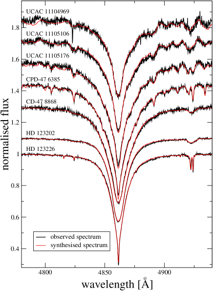
Figure 1: Comparison between the observed H$\beta$ line profile (thick lines) and synthetic line profile (thin lines) for seven stars observed with FLAMES/GIRAFFE. From top to bottom the stars here displayed are: UCAC 11104969 ($T_{\mathrm{eff}}$ = 7050 K), UCAC 11105106 ($T_{\mathrm{eff}}$ = 7500 K), UCAC 11105176 ($T_{\mathrm{eff}}$ = 8100 K), CPD-47 6385 ($T_{\mathrm{eff}}$ = 9350 K), CD-47 8868 ($T_{\mathrm{eff}}$ = 10400 K), HD 123202 ($T_{\mathrm{eff}}$ = 11400 K) and HD 123226 ($T_{\mathrm{eff}}$ = 12400 K). Profiles are vertically offset for display purpose.

Due to the very broad temperature range covered by the analysed stars, the hydrogen lines were used as both temperature and gravity indicators, because at lower temperatures hydrogen lines are more sensitive to temperature variations, while at higher temperatures gravity has the larger influence. This is also reflected on our error bars on the fundamental parameters.

Since with the fitting of the hydrogen line wings it was not always possible to derive simultaneously both $T_{\mathrm{eff}}$ and $\log g$, we adopted also two other spectroscopic indicators based on the analysis of metallic lines. In particular, $T_{\mathrm{eff}}$ was determined eliminating the correlation between line abundance and the line excitation potential ($\chi_{\mathrm{excit}}$) for a given ion/element and the surface gravity was determined with the ionisation balance of several elements. In particular we adopted mainly Fe lines to derive both $T_{\mathrm{eff}}$ and $\log g$ from metallic lines, adopting then Ti, Ca and Si lines (the latter for the hotter stars of the sample) as secondary indicators. Given the fact that the number of measurable lines decreases with increasing ${\upsilon}\sin i$, for stars with a high projected rotational velocity we ended up adopting only Fe lines.

Non-LTE effects might play an important role when measuring $\log g$ by imposing ionisation equilibrium. Fossati et al. (2009) concluded that for solar metallicity early-type stars non-LTE effects for Fe are most likely to be negligible. Mashonkina (2011) performed non-LTE calculations for Fe adopting the most complete iron model atom currently existing, and concluding that for A-type main-sequence stars non-LTE effects for FeI are less than 0.1 dex and negligible for FeII. Both Ti, Ca and Si are subject to non-LTE effects, but we considered these elements only as secondary parameter indicator, giving most of the weight to what derived from Fe lines.

For the cooler stars we were not able to apply the method based on line profile fitting of gravity-sensitive metal lines with developed wings, usually adopted to derive $\log g$ for late-type stars (see e.g. Fuhrmann et al. 1997), because the low resolution of the FLAMES/GIRAFFE spectra caused too heavy blending of those lines.

For stars with a low ${\upsilon}\sin i$  (${\upsilon}\sin i$$<30$ $\mathrm{km\,s}^{-1}$) LTE abundance analysis was based on equivalent widths, analysed with a modified version (Tsymbal 1996) of the WIDTH9 code (Kurucz 1993), while for fast rotating stars we derived the LTE abundances by line profile fitting of carefully selected lines (see Fossati et al. 2007, for more details).

The microturbulence velocity ($\upsilon_{\mathrm{mic}}$) was determined by minimising the correlation between equivalent width and abundance for several ions, for the slowly rotating stars for which it was possible to measure the line equivalent widths, or following the procedure described in Fossati et al. (2008b) for fast rotators, except for HD 123202, for which we were not able to measure $\upsilon_{\mathrm{mic}}$, which we then assumed to be 0.0 $\mathrm{km\,s}^{-1}$, with an uncertainty of 1.0 $\mathrm{km\,s}^{-1}$.

Table 2: Atmospheric parameters for the programme stars. The last six entries refer to SB2 stars for which only very few parameters could be estimated, and no abundance analysis was performed. The $\log g$ values given for the two components of HD 123225 are assumed and not measured, therefore it is not possible to give a realistic uncertainty to $T_{\mathrm{eff}}$ as well. Due to the very few measurable spectral lines, $\upsilon_{\mathrm{mic}}$ for HD 123202 is assumed.

Star	$T_{\mathrm{eff}}$		$\log g$		$\upsilon_{\mathrm{mic}}$		${\upsilon}\sin i$
name	[K]		[cgs]		[$\mathrm{km\,s}^{-1}$]		[$\mathrm{km\,s}^{-1}$]
HD 122983	10700 $\pm$	200	4.00 $\pm$	0.15	1.0 $\pm$	0.2	35 $\pm$	3
HD 123097	12000 $\pm$	300	3.96 $\pm$	0.10	1.5 $\pm$	0.6	133 $\pm$	5
HD 123182	10800 $\pm$	200	4.25 $\pm$	0.15	0.0 $\pm$	0.4	81 $\pm$	6
HD 123183	10900 $\pm$	250	4.05 $\pm$	0.15	0.6 $\pm$	0.8	275 $\pm$	14
HD 123184	10900 $\pm$	250	4.25 $\pm$	0.15	0.0 $\pm$	0.4	60 $\pm$	6
HD 123201B	11700 $\pm$	250	3.95 $\pm$	0.15	0.0 $\pm$	0.8	202 $\pm$	11
HD 123202	11400 $\pm$	250	3.70 $\pm$	0.15	0.0 $\pm$	1.0	301 $\pm$	17
HD 123226	12400 $\pm$	300	4.04 $\pm$	0.10	0.0 $\pm$	0.2	17 $\pm$	1
HD 123269	11600 $\pm$	250	3.94 $\pm$	0.15	0.0 $\pm$	0.2	25 $\pm$	2
CD-47 8868	10400 $\pm$	200	4.20 $\pm$	0.15	0.9 $\pm$	0.7	250 $\pm$	10
CD-47 8869	8400 $\pm$	200	3.60 $\pm$	0.20	1.2 $\pm$	0.7	230 $\pm$	10
CD-47 8889	10300 $\pm$	200	4.15 $\pm$	0.15	0.5 $\pm$	0.6	113 $\pm$	3
CD-47 8905	9700 $\pm$	200	4.10 $\pm$	0.20	1.6 $\pm$	0.4	160 $\pm$	6
CPD-47 6379	11000 $\pm$	250	4.30 $\pm$	0.15	1.7 $\pm$	0.6	136 $\pm$	7
CPD-47 6385	9350 $\pm$	200	4.12 $\pm$	0.20	1.6 $\pm$	0.3	55 $\pm$	5
UCAC 11104969	7050 $\pm$	150	4.00 $\pm$	0.20	1.4 $\pm$	0.9	260 $\pm$	15
UCAC 11105038	7650 $\pm$	200	4.00 $\pm$	0.20	3.4 $\pm$	0.4	85 $\pm$	5
UCAC 11105106	7500 $\pm$	200	4.00 $\pm$	0.20	2.5 $\pm$	0.6	195 $\pm$	10
UCAC 11105176	8100 $\pm$	200	4.00 $\pm$	0.20	1.8 $\pm$	0.4	125 $\pm$	7
UCAC 11105213	7600 $\pm$	200	4.00 $\pm$	0.20	1.9 $\pm$	0.3	57 $\pm$	3
UCAC 11105379	7700 $\pm$	200	4.00 $\pm$	0.20	2.1 $\pm$	0.2	44 $\pm$	2
HD 123225A	13100 $\pm$	-	3.8 $\pm$	-	$\pm$		12 $\pm$	1
HD 123225B	8000 $\pm$	-	4.0 $\pm$	-	$\pm$		20 $\pm$	2
NGC 5460 BB 338A	-						140 $\pm$	7
NGC 5460 BB 338B	-						$<$11 $\pm$	1
UCAC 11105152A	-						190 $\pm$	10
UCAC 11105152B	-						$<11$ $\pm$	1

Both the projected rotational velocity (${\upsilon}\sin i$) and ${\upsilon}_{\mathrm{r}}$ were determined by fitting synthetic spectra of several carefully selected lines on the observed spectrum.

Table 2 lists the fundamental parameters derived for each analysed star in NGC 5460. For some stars a preliminary spectral classification is given here for the first time on the basis of the derived $T_{\mathrm{eff}}$. The uncertainties of $T_{\mathrm{eff}}$ and $\log g$, listed in Table 2, were determined from the hydrogen line fitting, our main source for the parameter determination, therefore the given error bars take into account the quality of the observed spectra and the sensitivity of the hydrogen line wings to both $T_{\mathrm{eff}}$ and $\log g$ at different temperatures. Table 2 also shows that the uncertainties on $T_{\mathrm{eff}}$ and $\log g$ depend on the stellar ${\upsilon}\sin i$. This is due to the fact that we also adopted metallic lines to determine the atmospheric parameters and the precision with which we determined the element/ion abundances decreases with increasing ${\upsilon}\sin i$, for example because of the decreasing number of measurable lines for each ion.

The abundances obtained for each analysed star are shown in Table 3. The error bars are the standard deviations of the mean abundance derived from the individual line abundances, which include also the error bars in oscillator strengths determination given for the laboratory data (Fossati et al. 2009).

The standard deviation of the mean underestimates the actual abundance error bars, since uncertainties on the atmospheric parameters should also be taken into account. In particular for the fast rotating stars, the uncertainty on $\upsilon_{\mathrm{mic}}$ has a large impact on the total abundance uncertainty. For two stars with very similar atmospheric parameters, but different ${\upsilon}\sin i$ values (CPD-47 6385 and CD-47 8905) we determined the element abundances adopting model atmospheres for which we increased each atmospheric parameter one at a time, by an amount representative of the whole sample of stars: 250 K for $T_{\mathrm{eff}}$, 0.2 for $\log g$ and 0.7 $\mathrm{km\,s}^{-1}$ for $\upsilon_{\mathrm{mic}}$. Table 4 shows the results of this test. For the slow rotator, the abundance error bar is highly dominated by the uncertainty on $T_{\mathrm{eff}}$, while for the fast rotator, the uncertainty on $\upsilon_{\mathrm{mic}}$ plays a crucial role. In both cases the uncertainty on $\log g$ is almost negligible. This test also shows the dependency of the abundance error bars on the lines selected to perform the abundance analysis: for the slow rotator the abundance error bars of Mg, Ti and Ba, due to the uncertainty on $\upsilon_{\mathrm{mic}}$, are rather large. This is due to the fact that most of the lines selected to measure the abundance of these three elements are strong (e.g. the Mg triplet at $\lambda\lambda\sim$ 5167, 5172 and 5183), being therefore very sensitive to $\upsilon_{\mathrm{mic}}$ variations. Anyway, this effect is mitigated by the fact that for the slow rotators the uncertainty on $\upsilon_{\mathrm{mic}}$ is not as large as 0.7 $\mathrm{km\,s}^{-1}$, value chosen here to perform this test. Using the propagation theory in Table 4 we considered the situation where the determination of each fundamental parameter is an independent process, which in reality is not true, since there is a level of correlation between the various parameters. This makes the global uncertainties, given in columns five and nine of Table 4, upper limits. In conclusion, following the results of this test and of the ones performed by Fossati et al. (2008b) and Fossati et al. (2009), we can safely set a mean abundance uncertainty of 0.2 dex, for the slow rotators, which increases linearly with ${\upsilon}\sin i$, due to the increasing importance of the $\upsilon_{\mathrm{mic}}$ uncertainty in the total abundance error bar budget. The mean abundance error bars, adopted for each star, are shown in the last column of Table 3.

The impact of systematic uncertainties is different for different elements, but it is out of the scope of this work to go in such details, since here we are mainly interested in general trends and only marginally in the detailed abundance characteristics of each single star, which should require spectra with much higher resolution and signal-to-noise ratio (SNR), as demonstrated by Fossati et al. (2009).

Table 3: Element abundances, in $\log(N_{X}/N_{\rm tot})$, of the analysed cluster member stars. The estimated internal errors in units of 0.01 dex and the number of lines selected for each element are given in parenthesis. For comparison, the last row shows the solar abundances by Asplund et al. (2005). Abundances obtained from just one line have no error (-;1). The column labelled as ‘Uncertainty’ shows the abundance uncertainty for each star, calculated following Fossati et al. (2008b), and which is taken into account in the discussion of the results.

Star	He	C	O	Na	Mg	Al	Si	S
HD 122983	-2.00(-;1)		-3.41(-;1)		-5.22(-;1)	-6.19(-;1)	-4.41(-;1)
HD 123097	-0.90(-;1)				-4.55(36;3)	-5.85(-;1)	-4.54(01;2)
HD 123182	-1.48(-;1)		-3.41(-;1)		-4.56(01;2)	-5.43(-;1)	-4.58(09;2)
HD 123183			-3.40(11;4)		-4.30(16;3)		-4.37(19;2)
HD 123184	-0.90(05;3)	-3.47(-;1)	-3.28(01;3)		-4.35(16;5)	-5.56(-;1)	-4.39(10;4)
HD 123201B	-1.00(03;6)	-3.60(-;1)	-3.28(-;1)		-4.29(10;5)	-5.70(-;1)	-4.52(01;2)
HD 123202							-4.62(-;1)
HD 123226	-1.02(05;2)		-3.41(01;2)		-4.64(08;3)	-5.77(17;2)	-4.63(-;1)	-4.77(17;6)
HD 123269	-0.98(-;1)				-4.58(16;3)	-5.76(-;1)	-4.42(-;1)	-4.45(-;1)
CD-47 8868					-3.80(-;1)		-4.52(-;1)
CD-47 8869		-3.50(-;1)			-5.27(16;2)		-4.34(-;1)
CD-47 8889					-4.20(06;3)	-5.52(-;1)	-4.52(17;2)
CD-47 8905					-4.03(11;3)		-4.26(09;2)
CPD-47 6379					-4.10(28;3)		-4.77(45;2)
CPD-47 6385		-3.27(13;5)			-4.28(02;3)	-5.35(-;1)	-4.71(24;2)
UCAC 11104969		-3.47(-;1)			-5.11(32;2)		-3.58(-;1)
UCAC 11105038		-3.38(14;3)		-5.78(03;2)	-4.86(07;3)		-4.37(15;3)
UCAC 11105106				-6.13(06;2)	-4.62(21;4)		-4.09(21;2)
UCAC 11105176		-3.24(04;2)			-4.45(03;3)		-4.21(-;1)
UCAC 11105213		-3.49(12;3)		-5.69(04;2)	-4.87(06;3)		-4.27(13;3)	-4.37(-;1)
UCAC 11105379		-3.42(05;3)		-5.84(05;2)	-4.69(03;3)		-4.37(09;3)	-4.58(-;1)
sun	-1.11	-3.65	-3.38	-5.87	-4.51	-5.67	-4.53	-4.90
Star	Ca	Sc	Ti	V	Cr	Mn	Fe	Ni
HD 122983		-7.48(20;4)	-7.37(13;3)		-5.27(14;19)		-3.81(12;100)
HD 123097			-7.31(10;2)		-6.78(12;2)		-4.60(05;12)
HD 123182	-5.29(-;1)		-6.87(08;5)		-5.90(23;9)	-5.19(23;9)	-4.20(14;60)
HD 123183			-6.51(-;1)		-5.81(01;2)		-4.37(22;11)
HD 123184	-5.77(-;1)	-9.21(-;1)	-6.88(14;8)		-6.15(13;10)	-6.10(-;1)	-4.29(14;57)
HD 123201B			-6.54(18;5)		-5.99(14;4)		-4.47(14;20)
HD 123202					-5.94(10;2)		-4.50(07;5)
HD 123226			-7.27(-;1)		-6.63(12;6)		-4.75(15;54)	-5.86(-;1)
HD 123269			-7.26(25;2)		-6.48(13;9)		-4.57(16;60)	-5.76(-;1)
CD-47 8868			-7.04(15;2)		-6.40(25;4)		-4.25(21;13)
CD-47 8869	-5.35(-;1)	-9.68(-;1)	-6.67(08;2)		-6.58(11;4)	-6.82(-;1)	-4.50(10;15)
CD-47 8889			-7.07(13;3)		-6.16(09;5)		-4.27(17;22)
CD-47 8905			-7.00(28;4)		-6.39(10;4)		-4.43(15;21)
CPD-47 6379			-7.12(22;4)		-5.15(15;4)		-4.20(23;27)
CPD-47 6385	-5.30(09;4)	-8.81(04;3)	-6.85(13;12)		-6.04(09;17)	-5.99(03;2)	-4.38(09;59)	-5.55(30;2)
UCAC 11104969	-5.69(17;4)	-9.43(-;1)	-7.48(32;5)		-6.76(15;6)	-6.34(08;3)	-4.62(05;12)	-5.65(65;5)
UCAC 11105038	-6.23(09;8)	-9.17(19;3)	-7.64(17;19)		-6.50(15;16)	-6.83(14;3)	-5.08(13;91)	-6.09(18;9)
UCAC 11105106	-5.67(07;8)	-8.56(22;2)	-7.44(14;10)		-6.81(09;10)	-6.83(08;3)	-5.03(15;54)	-6.04(04;3)
UCAC 11105176	-5.86(06;4)	-8.82(11;2)	-6.97(19;7)		-6.33(08;10)	-6.35(17;3)	-4.80(12;61)	-5.74(16;5)
UCAC 11105213	-6.03(25;19)	-9.23(09;4)	-7.16(04;13)		-6.27(15;24)	-6.75(22;5)	-4.61(16;133)	-5.67(16;15)
UCAC 11105379	-5.89(14;15)	-9.11(11;4)	-7.22(05;15)	-7.76(-;1)	-6.39(12;22)	-6.78(12;4)	-4.74(16;129)	-6.11(18;14)
sun	-5.73	-8.99	-7.14	-8.04	-6.40	-6.65	-4.59	-5.81
Star	Cu	Zn	Sr	Y	Ba	Pr	Nd	Uncertainty
HD 122983					-8.64(-;1)	-7.57(20;3)	-7.43(10;8)	0.20
HD 123097								0.26
HD 123182				-9.81(-;1)	-9.09(-;1)			0.23
HD 123183								0.34
HD 123184			-9.34(-;1)					0.22
HD 123201B								0.30
HD 123202								0.36
HD 123226								0.20
HD 123269								0.20
CD-47 8868								0.33
CD-47 8869					-9.70(-;1)			0.32
CD-47 8889								0.25
CD-47 8905								0.28
CPD-47 6379								0.26
CPD-47 6385					-8.17(11;2)			0.21
UCAC 11104969				-8.64(03;2)	-8.55(-;1)			0.34
UCAC 11105038					-9.18(16;2)			0.23
UCAC 11105106		-6.79(-;1)			-9.63(-;1)			0.30
UCAC 11105176					-10.10(-;1)			0.26
UCAC 11105213		-7.15(-;1)		-9.64(16;3)	-8.51(16;2)			0.22
UCAC 11105379		-7.75(-;1)		-9.87(13;2)	-9.35(16;2)			0.21
sun	-7.83	-7.44	-9.12	-9.83	-9.87	-11.33	-10.59

Table 4: Error sources for the abundances of the chemical elements of CPD-47 6385 and CD-47 8905. Both stars have very similar atmospheric parameters ($T_{\mathrm{eff}}$$\sim$9500 K, $\log g$$\sim$4.1 and $\upsilon_{\mathrm{mic}}$$\sim$1.6 $\mathrm{km\,s}^{-1}$), but rather different ${\upsilon}\sin i$ values, as shown in the second table line. Columns 2$-$4 and 6$-$8 give the variation in abundance estimated by increasing $T_{\mathrm{eff}}$ by 250 K, $\log g$ by 0.1 dex, and $\upsilon_{\mathrm{mic}}$ by 0.7 $\mathrm{km\,s}^{-1}$, respectively. Columns 5 and 9 give the mean error calculated applying the standard error propagation theory on the systematic uncertainties given in Col. 2$-$4 and 6$-$8, i.e., $\sigma_{\rm abn}^{2}$ (syst.) = $\sigma_{\rm abn}^{2}$ ($T_{\mathrm{eff}}$) + $\sigma_{\rm abn}^{2}$ ($\log g$) + $\sigma_{\rm abn}^{2}$ ($\upsilon_{\mathrm{mic}}$).

	CPD-47 6385				CD-47 8905
	${\upsilon}\sin i$=55 $\mathrm{km\,s}^{-1}$				${\upsilon}\sin i$=160 $\mathrm{km\,s}^{-1}$
El.	$\sigma_{\rm abn}$($T_{\mathrm{eff}}$)	$\sigma_{\rm abn}$($\log g$)	$\sigma_{\rm abn}$($\upsilon_{\mathrm{mic}}$)	$\sigma_{\rm abn}$(syst.)	$\sigma_{\rm abn}$($T_{\mathrm{eff}}$)	$\sigma_{\rm abn}$($\log g$)	$\sigma_{\rm abn}$($\upsilon_{\mathrm{mic}}$)	$\sigma_{\rm abn}$(syst.)
	(dex)	(dex)	(dex)	(dex)	(dex)	(dex)	(dex)	(dex)
C	0.15	$-$0.04	$-$0.01	0.15
Mg	0.21	$-$0.07	$-$0.15	0.27	0.31	$-$0.07	$-$0.28	0.42
Al	0.00	0.06	$-$0.03	0.07
Si	0.09	$-$0.03	$-$0.04	0.10	0.05	$-$0.01	$-$0.06	0.08
Ca	0.25	$-$0.04	$-$0.09	0.27
Sc	0.14	0.04	$-$0.03	0.15
Ti	0.08	0.01	$-$0.17	0.19	0.17	0.05	$-$0.31	0.36
Cr	0.13	0.03	$-$0.08	0.16	0.17	0.06	$-$0.19	0.26
Mn	0.23	$-$0.01	$-$0.03	0.23
Fe	0.13	0.00	$-$0.08	0.15	0.09	0.04	$-$0.16	0.19
Ni	0.10	$-$0.03	0.00	0.10
Ba	0.26	$-$0.07	$-$0.48	0.55

4 The impact of systematic errors

The scattering of the element abundance obtained from different lines provides only a lower limit for the actual error in the abundance determination. Systematic effects introduced by the normalisation to the continuum, and inaccurate $T_{\mathrm{eff}}$ and $\log g$ estimates may have a large impact. To explore the reliability of the error estimates of Table 3 we re-analysed a number of stars in a completely independent way, using the Zeeman (Landstreet 1988; Wade et al. 2001) spectrum synthesis code. This ‘secondary’ analysis helps to ensure our results and estimated uncertainties are robust.

The Zeeman code performs polarised radiative transfer, under the assumption of LTE, using plane-parallel model atmospheres. Input LTE model atmospheres were calculated using atlas9 (Kurucz 1993), assuming solar abundances, which are a reasonable starting point as none of the stars in NGC 5460 show extreme chemical peculiarities. Input atomic data was drawn from the VALD database, using an ‘extract stellar’ request, with effective temperature and surface gravity tailored to the specific star, and solar abundances.

Initial values for temperatures and surface gravities were found by fitting synthetic Balmer lines to the observations. These values were confirmed, and when possible refined, by fitting metallic lines with a range of ionisation states and excitation potentials. The Balmer line fitting was performed by eye, though the metallic line fitting was done using $\chi^{2}$ minimisation.

Abundances, ${\upsilon}\sin i$ and $\upsilon_{\mathrm{mic}}$ were determined by fitting a synthetic spectrum to the observation, using a Levenberg-Marquardt $\chi^{2}$ minimisation procedure. This was performed for 3 segments of spectrum between 100 Å and 500 Å long in the 4500–6000 Å region. The final best fit values reported here are averages over the individual segments. Uncertainties are generally taken to be the standard deviation. For elements with less then $\sim 3$ useful lines, an uncertainty was estimated by eye, taking into account the scatter between lines, blending, and potential normalisation errors.

Best fit results for the stars analysed with this method are presented in Table 5. Figure 2 shows the histogram of the difference of the abundances obtained with the secondary and the standard analysis, divided by the error bar of the standard analysis (last column of Table 3). Generally the results are very consistent, with the abundances being within uncertainty of each other, at least within a $1.5\sigma$ limit.

This secondary analysis supports also the conclusion that HD 123182 is chemically peculiar. A large Mn overabundance is confirmed, though no Sc or Hg abundances could be derived. Our secondary analysis confirms also that HD 123183 is a chemically normal star, with a very high ${\upsilon}\sin i$, despite one published marginal magnetic field detection. In both HD 123201B and HD 123184 discrepancies in ${\upsilon}\sin i$ were again detectable for lines with high excitation potentials, particularly He lines. The secondary analysis confirms both these stars are chemically normal.

Table 5: Best fit parameters from the comparison analysis with Zeeman. Chemical abundances are in units of $\log(N_{X}/N_{tot})$. Elements marked with an asterisk are based on less than $\sim 3$ useful lines and have uncertainties estimated by eye.

	HD 123182	HD 123183	HD 123184	HD 123201B	HD 123226	CPD-476379	CPD-476385
$T_{\mathrm{eff}}$ $[$K$]$	$10800\pm 300$	$10500\pm 700$	$10900\pm 120$	$12000\pm 450$	$12140\pm 160$	$10100\pm 300$	$9360\pm 150$
$\log g$ $[$cgs$]$	$4.25\pm 0.2$	$4.3\pm 0.3$	$4.35\pm 0.2$	$4.2\pm 0.3$	$4.27\pm 0.1$	$4.15\pm 0.2$	$4.12\pm 0.2$
${\upsilon}\sin i$ $[$$\mathrm{km\,s}^{-1}$$]$	$81\pm 4$	$270\pm 15$	$63.1\pm 1.5$	$203\pm 6$	$18.1\pm 1.0$	$140\pm 8$	$56.1\pm 2.5$
$\upsilon_{\mathrm{mic}}$ $[$$\mathrm{km\,s}^{-1}$$]$	$\sim 0$	$\sim 0$	$0.4\pm 0.22$	$\sim 0$	$0.5\pm 0.5$	$1.02\pm 0.45$	$1.8\pm 0.2$
Vr $[$$\mathrm{km\,s}^{-1}$$]$	$-1\pm 6$	$-18\pm 20$	$-14\pm 1$	$-25\pm 13$	$-12\pm 1$	$-30\pm 3$	$-21\pm 1$
He	$-1.48\pm 0.4$ *		$-0.9\pm 0.2$ *	$-1.05\pm 0.2$ *	$-0.9\pm 0.2$ *
C			$-3.4\pm 0.2$ *
O	$-3.54\pm 0.1$	$-3.5\pm 0.2$ *	$-3.3\pm 0.12$	$-3.45\pm 0.2$ *	$-3.57\pm 0.2$ *	$-3.4\pm 0.21$	$-3.3\pm 0.15$ *
Na							$-5.48\pm 0.2$ *
Mg	$-4.5\pm 0.2$	$-4.9\pm 0.4$ *	$-4.56\pm 0.14$	$-4.49\pm 0.24$	$-4.87\pm 0.06$	$-4.47\pm 0.17$	$-4.40\pm 0.05$
Al	$-6.1\pm 0.5$ *		$-5.6\pm 0.2$ *	$-5.85\pm 0.4$ *	$-5.65\pm 0.15$	$-5.68\pm 0.3$ *
Si	$-4.7\pm 0.2$	$-4.5\pm 0.2$ *	$-4.4\pm 0.11$	$-4.71\pm 0.27$	$-4.57\pm 0.08$	$-4.85\pm 0.15$ *	$-4.59\pm 0.1$ *
S			$-4.4\pm 0.3$ *		$-4.92\pm 0.3$ *
Ca	$-5.68\pm 0.4$ *		$-5.52\pm 0.27$			$-5.67\pm 0.3$ *	$-5.45\pm 0.15$
Sc			$-8.8\pm 0.1$			$-8.48\pm 0.2$ *	$-8.81\pm 0.09$
Ti	$-6.88\pm 0.1$	$-7.3\pm 0.4$ *	$-7.16\pm 0.12$	$-7.26\pm 0.15$	$-7.4\pm 0.1$	$-6.87\pm 0.08$	$-6.88\pm 0.06$
V			$-8.4\pm 0.4$ *
Cr	$-6.24\pm 0.1$	$-6.9\pm 0.4$ *	$-5.99\pm 0.11$	$-6.67\pm 0.2$	$-6.53\pm 0.05$	$-5.53\pm 0.11$	$-6.21\pm 0.14$
Mn	$-5.52\pm 0.1$		$-6.4\pm 0.3$ *		$-6.72\pm 0.3$ *
Fe	$-4.31\pm 0.1$	$-4.4\pm 0.2$	$-4.41\pm 0.14$	$-4.66\pm 0.19$	$-4.73\pm 0.05$	$-4.16\pm 0.05$	$-4.35\pm 0.15$
Ni
Cu
Zn
Y			$-9.6\pm 0.4$ *				$-9.19\pm 0.4$ *
Ba			$-9.6\pm 0.4$ *				$-8.85\pm 0.4$ *

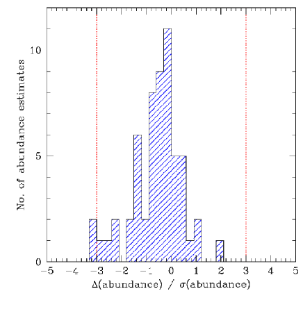
Figure 2: Histogram of the difference of the abundances obtained with the secondary and the standard analysis, divided by the error bar of the standard analysis, listed in the last column of Table 3. The dashed lines correspond to a 3-$\sigma$ difference.

5 Results

Our ${\upsilon}_{\mathrm{r}}$ measurements allowed us to derive the mean cluster radial velocity: $-17.9\pm 5.2$ $\mathrm{km\,s}^{-1}$, obtained without taking into account the double line spectroscopic binaries (SB2) stars. This value agrees rather well with $-12.70\pm 2.18$ $\mathrm{km\,s}^{-1}$, published by Kharchenko et al. (2005), in particular taking into account that the latter value is the average of the ${\upsilon}_{\mathrm{r}}$ of only three stars.

We cannot exclude that some of the analysed stars are single line spectroscopic binaries (SB1), but this was impossible to establish with the available spectra.

In the following we describe more in detail the results obtained for the most interesting objects.

5.1 HD 122983

The star HD 122983 was observed by Bagnulo et al. (2006) to measure the longitudinal magnetic field, but no field was detected. The abundance pattern shows that HD 122983 is a He-weak star, but it was not possible to determine the kind of chemical peculiarity (e.g. HgMn star). Manganese lines are too shallow to be measured and none of the covered mercury line is visible. A spectrum covering the spectral region around 3900 Å would be extremely valuable to detect the presence of Hg overabundance (Hubrig & Mathys 1996). We looked also for the overabundance of elements characteristic of HgMn stars, such as P and Xe, but without results.

5.2 HD 123182

The abundance pattern of HD 123182 reveals that the star is most likely a mild He-weak star, in particular it could be a hot Am star or a cool HgMn star. Sc lines are too weak to be measurable, so it is not possible to say whether it is underabundant or not. The not extreme overabundance of Cr and Fe (as expected for the rather high ${\upsilon}\sin i$), and the fact that Hg, P and Xe are not visible (although lines would be covered) are in agreement with an Am classification. On the other hand the clear Mn overabundance would tend more to a HgMn classification. On the basis of the available data we can only conclude that HD 123182 is a He-weak star of an unclear type. This star could also be a single line spectroscopic binary, due to the high radial velocity, compared to the one of the other cluster stars.

5.3 HD 123183

The star HD 123183 was observed with FORS1 by Bagnulo et al. (2006) who published a marginal magnetic field detection of $\langle Bz\rangle=-440\pm 146$ G. The abundance pattern does not reveal any chemical peculiarity that could strengthen this detection. The very high ${\upsilon}\sin i$ of $275\pm 14$ $\mathrm{km\,s}^{-1}$ also goes against a classification of this object as chemically peculiar. For this reason we conclude that HD 123183 is a chemically ‘normal’ early-type star. Given the very high ${\upsilon}\sin i$, it would be very valuable to perform new magnetic field measurements.

5.4 HD 123225

The FLAMES/UVES observations of HD 123225 revealed that this is a SB2 system, where both components appear to have a rather low ${\upsilon}\sin i$. The spectral lines of the two components are well separated: ${\upsilon}_{\mathrm{r}}$ of the first component is $\sim-$2 $\mathrm{km\,s}^{-1}$, while ${\upsilon}_{\mathrm{r}}$ of the second component is $\sim-53$ $\mathrm{km\,s}^{-1}$. With only one available spectrum it was not possible to perform a precise abundance analysis, but the large separation of the two components allowed to roughly estimate their $T_{\mathrm{eff}}$: 13100 K for the primary and 8000 K for the secondary star. These values were obtained from a fit of synthetic spectra on the observed H$\beta$ profile (see Fig. 3), taking into account the expected relative difference in flux due to the different stellar radii of the two components and assuming that both are main sequence stars ($\log g$ was set to 3.8 for the hotter star and to 4.0 for the cooler star).

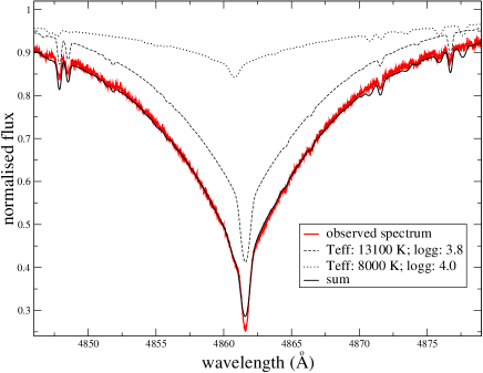
Figure 3: Fit of the observed H$\beta$ line profile for HD 123225. The red line shows the observed spectrum, while the dashed and dotted lines are the synthetic spectra of the two components assuming $T_{\mathrm{eff}}$ and $\log g$ of 13100 K and 3.8 for the hotter star and 8000 K ad 4.0 for the cooler star. The black solid line shows the sum of the two synthetic spectra.

The ${\upsilon}\sin i$ value of the primary star is $\sim$11 $\mathrm{km\,s}^{-1}$, while for the secondary star we derived a ${\upsilon}\sin i$ value of $\sim$20 $\mathrm{km\,s}^{-1}$. Given the roughly determined $T_{\mathrm{eff}}$ of the two components and their ${\upsilon}\sin i$, it is possible that both stars developed chemical peculiarities and in particular HgMn peculiarities for the primary star and Am peculiarities for the secondary star. To reveal whether HgMn peculiarities are present in the primary star, we looked for typical signatures present in HgMn stars. The spectrum reveals strong Mn lines in addition to evidences of Hg lines, allowing to conclude that the primary component is a HgMn star. This conclusion is strengthened by the fact that we found several strong lines of both Ne, P and Xe, typical of HgMn stars. For the secondary star it was not possible to determine whether it shows Am chemical peculiarities since the Sc lines are too shallow to be visible. In any case, the fact that the star seems to have Fe lines compatible with a solar iron abundance, let us believe that the secondary component is not an Am star.

HD 123225 was observed with FORS1 by Bagnulo et al. (2006) and no magnetic field was detected.

5.5 HD 123201B and HD 123184

The stars HD 123201B and HD 123184 are both chemically ‘normal’ early-type stars and share the common property of showing a different ${\upsilon}\sin i$ for the high $\chi_{\mathrm{excit}}$ lines, compared to the other spectral lines. The ${\upsilon}\sin i$ of HD 123201B, measured on low $\chi_{\mathrm{excit}}$ lines, is $\sim$202 $\mathrm{km\,s}^{-1}$, while He lines are best fit with a ${\upsilon}\sin i$ of $\sim$150 $\mathrm{km\,s}^{-1}$. The same occurs for HD 123184, for which ${\upsilon}\sin i$ is $\sim$60 $\mathrm{km\,s}^{-1}$, but He lines are best fit with a ${\upsilon}\sin i$ of $\sim$50 $\mathrm{km\,s}^{-1}$.

Figure 4 shows the comparison between the observed spectrum and two synthetic line profiles with ${\upsilon}\sin i$ = 60 and 50 $\mathrm{km\,s}^{-1}$ in the region of the FeII line at $\sim$5018 Å and of the HeI multiplet at $\sim$ 5875 Å for HD 123184. The plot shows that for the HeI multiplet the adopted stellar ${\upsilon}\sin i$ of 60 $\mathrm{km\,s}^{-1}$is far too high, while a ${\upsilon}\sin i$ of 50 $\mathrm{km\,s}^{-1}$ is necessary to fit the observed line profile. In contrast, the region around the FeII line shows that a ${\upsilon}\sin i$ of 60 $\mathrm{km\,s}^{-1}$  is required to fit this line. For both stars the He abundance was measured with the ${\upsilon}\sin i$ determined for the He lines.

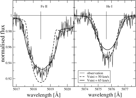
Figure 4: Comparison between the observed spectrum (thin line) and synthetic spectra calculated with ${\upsilon}\sin i$ = 60 $\mathrm{km\,s}^{-1}$ (thick line) and ${\upsilon}\sin i$ = 50 $\mathrm{km\,s}^{-1}$ (thick dashed line) in the region of the FeII line at $\sim$5018 Å  (left plot) and of the HeI multiplet at $\sim$5875 Å  (right plot), for HD 123184.

This effect is most likely a consequence of the fact that both stars are fast rotators with a rather small inclination of the rotation axis relative to the line of sight, leading to a temperature difference between the poles (hotter) and the equator (cooler) (von Zeipel 1924).

5.6 UCAC 11105038

This is an A-type star with a ${\upsilon}\sin i$ of 85$\pm$5 $\mathrm{km\,s}^{-1}$ and a relatively high $\upsilon_{\mathrm{mic}}$ of about 3.4 $\mathrm{km\,s}^{-1}$. Both ${\upsilon}\sin i$ and $\upsilon_{\mathrm{mic}}$ could indicate a possible Am chemical peculiarity of this star, in particular ${\upsilon}\sin i$ is below 90 $\mathrm{km\,s}^{-1}$ (Charbonneau & Michaud 1991), and $\upsilon_{\mathrm{mic}}$ is typical of Am stars (Landstreet 1998; Fossati et al. 2008b). Both Ca and Sc abundances are below the solar values, as well as the Ba overabundance is indicative of Am chemical peculiarities, but the underabundance of the Fe-peak elements goes against an Am classification.

6 Discussion

6.1 Abundance patterns in NGC 5460: from F- to B-type stars

Figure 5 shows the comparison among the mean abundance pattern obtained for B-, A- and F-type stars here analysed and considered members of the cluster. The error bars are the standard deviation from the mean abundance. In the whole sample, after the assignment of the cluster membership and binarity, only one F-type single star, UCAC 11104969, was left in the sample, therefore the mean abundance of the F-type stars corresponds to the abundance pattern of UCAC 11104969.

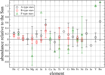
Figure 5: Comparison between the mean abundances obtained for B-, A- and F-type stars indicated by an open square, circle and triangle respectively. The error bars are the standard deviations from the calculated mean abundances. The abundance patter of the mean F-type stars is corresponds to the abundance pattern of UCAC 11104969, since it is the only F-type stars of the sample with measured abundances.

Figure 5 shows that the three abundance patterns are quite similar and concentrated around solar values except for a sulfur overabundance, which cannot be ascribed to non-LTE effects (Fossati et al. 2007), and for an apparent Am peculiarity of some elements in UCAC 11104969, excluded by the high ${\upsilon}\sin i$ value (260$\pm$15 $\mathrm{km\,s}^{-1}$).

An important result of this work is the estimation of the cluster metallicity ($Z$), spectroscopically never measured before. For the elements that most affect $Z$, such as C, O, Si, and Fe, we registered a rather good agreement among the three stellar types, with the exception of the Si abundance of UCAC 11104969, which was not taken into account in the determination of $Z$. Since the cluster metallicity should be calculated on the basis of the abundances of the cool stars (more mixed) and that only one F-type star is present in our sample, we decided to derive $Z$ from the mean abundance of UCAC 11104969 and of the A-type stars with $T_{\mathrm{eff}}$ $\leq$ 8500 K.

The cluster metallicity ($Z$) is defined as follows:

$$Z_{\rm cluster}=\frac{\sum_{a\geq 3}m_{a}10^{\log(N_{a}/N_{tot})}}{\sum_{a\geq 1}m_{a}10^{\log(N_{a}/N_{tot})}},$$ (1)

where $a$ is the atomic number of an element with atomic mass m_a. Making use of the mean abundances, we derived a metallicity of $Z$ = 0.014 $\pm$ 0.003, consistent with the solar $Z$ ($Z$=0.012, Asplund et al. 2005), adopting solar abundances by Asplund et al. (2005) for all elements that were not analysed.

The $Z$ value adopted by several other authors and used to characterise isochrones is calculated with the following approximation:

$$Z_{\mathrm{c}luster}\simeq 10^{([Fe/H]_{\mathrm{F}stars}-[Fe/H]_{\odot})}\cdot Z_{\odot}\ ,$$ (2)

assuming $Z_{\odot}$=0.019, which is favored by the theoretical stellar structure models based on (Anders & Grevesse 1989) solar abundances. We recalculated the $Z$ value of NGC 5460, according to this approximation, obtaining $Z$ = 0.013${}^{+0.008}_{-0.005}$, only about consistent with a solar metallicity. This value was derived from the mean Fe abundance of the seven stars taken into account ([Fe/H] = $-0.18\pm$0.22 dex). We believe that a solar metallicity would be anyway more appropriate for NGC 5460. The Fe underabundance of $-$0.18 dex is biased by two stars (out of a sample of seven) which show a considerable underabundance ([Fe/H]$\sim-$0.46 dex). On the other hand, for the other five stars the iron abundance is [Fe/H]=$-$0.06$\pm$0.12 dex, which leads to $Z$ = 0.017${}^{+0.005}_{-0.004}$, that, given the uncertainties, is perfectly consistent with a solar metallicity. In addition, Fig. 5 shows that the mean Fe abundance of the analysed cluster stars is well centered around the solar value.

6.2 HR diagram

With the obtained effective temperatures and the magnitudes provided by Claria et al. (1993), we built the Hertzsprung-Russell (HR) diagram of the cluster (Fig. 6), adopting a distance modulus of 9.44 mag, a reddening of 0.092 mag (both values given by WEBDA, Mermillod & Paunzen 2003), and the bolometric correction from Balona (1994).

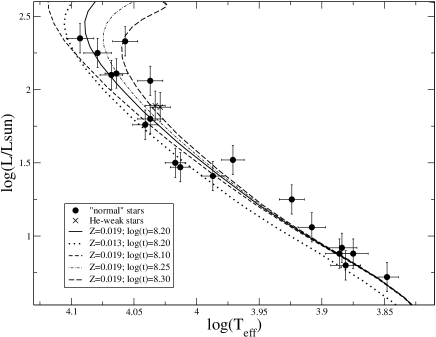
Figure 6: Hertzsprung-Russell diagram of NGC 5460. The crosses and filled circles show the position on the HR diagram for the chemically peculiar and chemically normal stars, respectively. The error bar in luminosity is 0.10 dex. The full and dotted lines show isochrones from Marigo et al. (2008) for an age of $\log t$ = 8.20 with solar metallicity ($Z$ = 0.019) and $Z$ = 0.013, respectively. The short dashed, thin dot-dashed line and long dashed line show solar metallicity isochrones of three different ages: $\log t$ = 8.10, 8.25 and 8.30, respectively.

Luminosities are listed in Table 6. With a distance modulus uncertainty of 0.20 mag, an uncertainty in the bolometric correction of about 0.07 mag, and a reddening uncertainty of 0.01 mag, we estimate the typical uncertainty in $M_{\mathrm{bol}}$ being about 0.28 mag, corresponding to an uncertainty in $\log L/L_{\odot}$ of about 0.10 dex.

Table 6: $\log L/L_{\odot}$, $\log$$T_{\mathrm{eff}}$, M/M_⊙ and fractional age ($\tau$) with associated error bars for the stars of the NGC 5460 open cluster.

Star	$\log L/L_{\odot}$	$\log$$T_{\mathrm{eff}}$	$M/M_{\odot}$		$\tau$
HD 122983	1.88	4.029	2.76 $\pm$	0.14	0.37 $\pm$	0.15
HD 123097	2.25	4.079	3.40 $\pm$	0.17	0.67 $\pm$	0.27
HD 123182	1.89	4.033	2.80 $\pm$	0.14	0.38 $\pm$	0.16
HD 123183	1.80	4.037	2.73 $\pm$	0.14	0.36 $\pm$	0.15
HD 123184	2.06	4.037	3.02 $\pm$	0.21	0.48 $\pm$	0.19
HD 123201B	2.10	4.068	3.17 $\pm$	0.16	0.55 $\pm$	0.22
HD 123202	2.33	4.057	3.45 $\pm$	0.24	0.70 $\pm$	0.28
HD 123226	2.35	4.093	3.60 $\pm$	0.18	0.79 $\pm$	0.32
HD 123269	2.11	4.064	3.15 $\pm$	0.16	0.54 $\pm$	0.22
CD-47 8868	1.50	4.017	2.30 $\pm$	0.16	0.22 $\pm$	0.09
CD-47 8869	1.25	3.924	1.94 $\pm$	0.14	0.14 $\pm$	0.05
CD-47 8889	1.47	4.013	2.35 $\pm$	0.16	0.23 $\pm$	0.09
CD-47 8905	1.41	3.987	2.20 $\pm$	0.11	0.19 $\pm$	0.08
CPD-47 6379	1.76	4.041	2.71 $\pm$	0.14	0.35 $\pm$	0.14
CPD-47 6385	1.52	3.971	2.27 $\pm$	0.16	0.21 $\pm$	0.09
UCAC 11104969	0.72	3.848	1.48 $\pm$	0.07	0.06 $\pm$	0.03
UCAC 11105038	0.92	3.884	1.66 $\pm$	0.08	0.09 $\pm$	0.04
UCAC 11105106	0.88	3.875	1.60 $\pm$	0.08	0.08 $\pm$	0.03
UCAC 11105176	1.06	3.908	1.78 $\pm$	0.09	0.11 $\pm$	0.04
UCAC 11105213	0.80	3.881	1.59 $\pm$	0.08	0.08 $\pm$	0.03
UCAC 11105379	0.88	3.886	1.64 $\pm$	0.08	0.08 $\pm$	0.03

Two stars of our sample, HD 122983 and HD 123183, are included in the work by Landstreet et al. (2007) and there is a good agreement between the obtained $\log L/L_{\odot}$ and $M/M_{\odot}$ values, where the small differences are due to the adoption of a different source for the stellar magnitudes. We adopted the magnitudes given by Claria et al. (1993), while Landstreet et al. (2007) adopted the magnitudes published by Claria (1971).

Figure 6 shows that assuming a metallicity of 0.013 would have little impact on the estimate of the cluster age, but just of the cluster distance, decreasing it by about 100 pc. Therefore, we can safely conclude that the distance of the cluster is within the range 670–770 pc. Out HR diagram allows also to better constrain the cluster age. The age of the solar metallicity isochrone fitting the cluster main sequence is $\log t$=8.10, which we can then consider as the minimum cluster age. The maximum age instead depends strongly on which stars of the upper main sequence are blue strugglers. If none of our analysed cluster stars is a blue struggler, the maximum cluster age is most likely to be $\log t$=8.25, while if HD 123226 (the hottest star in our sample) is a blue struggler the maximum cluster age is more likely to be $\log t$=8.30. On the basis of these considerations, our best estimate of the cluster age is $\log t$=8.20$\pm$0.10, in comparison to $\log t$=8.20$\pm$0.20 previously given by Ahumada & Lapasset (2007)).

6.3 Abundances vs. $T_{\mathrm{eff}}$ and ${\upsilon}\sin i$

From Fig. 7 to Fig. 9 we display the abundances of chemical elements versus $T_{\mathrm{eff}}$.

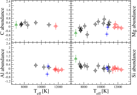
Figure 7: Abundances relative to the Sun (Asplund et al. 2005) of C, Mg, Al and Si as a function of $T_{\mathrm{eff}}$ for B-type stars (open squares), A-type stars (open circles), F-type stars (open triangles) and He-weak stars (crosses).

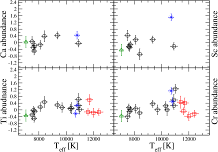
Figure 8: Same as Fig. 7, but for Ca, Sc, Ti and Cr.

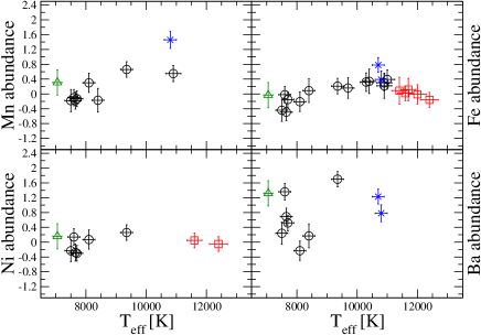
Figure 9: Same as Fig. 7, but for Mn, Fe, Ni and Ba.

For some elements, such as Mg and Fe, it is possible to notice a correlation of the abundances with $T_{\mathrm{eff}}$, with an abundance increase with $T_{\mathrm{eff}}$ up to $T_{\mathrm{eff}}$$\sim$10500 K and an abundance decrease for higher temperatures. A linear fit shows that these correlations are significant for both Mg and Fe (see Table 7).

Table 7: Correlations and relative uncertainties of the Mg and Fe element abundance as a function of $T_{\mathrm{eff}}$, in two temperature ranges: $T_{\mathrm{eff}}$$<$10500 K and $T_{\mathrm{eff}}$$>$10500 K. The last two rows show the correlations obtained for Mg and Fe from the Erspamer & North (2003) data.

Element	$T_{\mathrm{eff}}$	slope	$\sigma_{slope}$
Mg	$<$10500 K	3.04$\times$10-4	0.42$\times$10-4
Mg	$>$10500 K	$-$1.71$\times$10-4	1.08$\times$10-4
Fe	$<$10500 K	1.88$\times$10-4	0.47$\times$10-4
Fe	$>$10500 K	$-$4.03$\times$10-4	0.82$\times$10-4
Mg	$<$10500 K	7.23$\times$10-5	1.80$\times$10-5
Fe	$<$10500 K	1.21$\times$10-4	0.21$\times$10-4

These correlations could in principle not be real, but due to other factors, such as $\upsilon_{\mathrm{mic}}$, $\log g$ and ${\upsilon}\sin i$. We excluded that both $\upsilon_{\mathrm{mic}}$ and $\log g$ produced such trends, since the abundance uncertainties take into account the $\upsilon_{\mathrm{mic}}$ uncertainty, and the effect of $\log g$ variations on the abundances is much smaller than the deviations obtained here. In addition, we did not find any clear correlation between the abundances and ${\upsilon}\sin i$, as shown in Fig. 10, except for a decreasing Ba abundance with increasing ${\upsilon}\sin i$ up to ${\upsilon}\sin i$ values of about 125 $\mathrm{km\,s}^{-1}$, in agreement with predictions by Turcotte & Charbonneau (1993). We find also unlikely that our LTE approximation could be the source of the abundance correlations with $T_{\mathrm{eff}}$, since for both Mg and Fe the expected non-LTE corrections are small (Przybilla et al. 2001; Fossati et al. 2009) and their dependence on $T_{\mathrm{eff}}$ is not expected to be as pronounced as shown by our results.

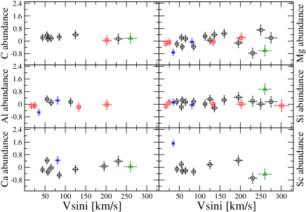
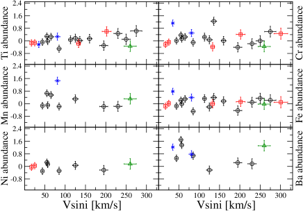
Figure 10: Abundances relative to the Sun (Asplund et al. 2005) as a function of ${\upsilon}\sin i$ for B-type stars (open squares), A-type stars (open circles), F-type stars (open triangles) and He-weak stars (crosses).

As further check for the obtained abundance correlations with $T_{\mathrm{eff}}$, we looked for similar trends in other consistently analysed sample of stars covering a large temperature range. Erspamer & North (2003) analysed the spectra of 140 A- and F-type stars, present in the ELODIE archive, obtaining for each star fundamental parameters and abundances of several elements. Figure 11 shows a comparison between the results we obtained in NGC 5460 and what published by Erspamer & North (2003) for Mg and Fe.

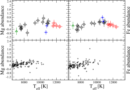
Figure 11: Comparison between the results obtained in this work (upper panels) and by Erspamer & North (2003) (lower panels), for Mg (on the left side) and Fe (on the right side). B-type stars are denoted with open squares, A-type stars with open circles, F-type stars with open triangles and He-weak stars with crosses.

We register an agreement for both elements, in particular for Fe (see Table 7), although the trends appear less pronounced in the results published by Erspamer & North (2003). Unfortunately the sample of stars analysed by Erspamer & North (2003) did not cover stars with temperatures higher than 10500 K, so that it was not possible to check the presence of the abundance drop, present in our results.

Diffusion processes could be responsible for the obtained abundance correlations with $T_{\mathrm{eff}}$. With the increase of the effective temperature the hydrogen and helium ionisation zones shift more and more towards the stellar surface, and as a consequence they become thinner and less turbulent. In this way diffusion processes become more and more effective. For example, it is well known that Ba is overabundant in early-type stars, which is a clear signature of an influence of diffusion even in chemically normal stars (Fossati et al. 2009). Another example is the presence of a correlation between strontium and oxygen or strontium and magnesium, obtained for chemically normal B-type stars by Hempel & Holweger (2003) (strontium is radiatively driven outwards, Mg and O sink down).

The efficiency of diffusion processes is reduced by rotation. In particular, simulations carried out by Turcotte & Charbonneau (1993) show that for rotational velocities higher than 125 $\mathrm{km\,s}^{-1}$ the envelope is completely mixed. This would suggest that correlations between abundances of diffusion indicator elements (such as Sr, O, Mg, and Ba) and ${\upsilon}\sin i$ should be obtained even for chemically normal star. But correlations between abundance and ${\upsilon}\sin i$ are not found here, except for Ba, one of the diffusion indicators, for which the abundance decreases mildly with ${\upsilon}\sin i$, up to ${\upsilon}\sin i$ values of $\sim$125 $\mathrm{km\,s}^{-1}$, in agreement with what predicted by Turcotte & Charbonneau (1993). Probably a much larger sample of stars, which includes chemically normal low ${\upsilon}\sin i$ stars could show the presence or not of these correlations.

7 Conclusions

We obtained low and mid-resolution spectra of several stars in the field of the NGC 5460 open cluster with the FLAMES spectrograph at the ESO/VLT, and we selected 24 probable cluster members with $T_{\mathrm{eff}}$$>7000$. This cluster was never previously spectroscopically studied.

We calculated the fundamental parameters and performed a detailed abundance analysis for all the stars of the sample, except for three objects (HD 123225, Cl NGC 5460 BB 338, and UCAC 11105152), which turned out to be double line spectroscopic binaries. Two stars, HD122983 and HD 123182, are He-weak stars, and we suspect that the hotter component of the HD 123225 SB2 system is a HgMn chemically peculiar star. Bagnulo et al. (2006) obtained a marginal magnetic field detection for HD 123183, but the star has remarkably high ${\upsilon}\sin i$ for an Ap star, and no clear chemical peculiarities.

The mean abundance pattern obtained for B-, A- and F-type stars considered members of the cluster concentrate around solar values. We determined the cluster metallicity from the cooler stars of our sample ($T_{\mathrm{eff}}$$<$8500 K). The resultant metallicity is $Z=0.014\pm 0.003$. We rederived $Z$ also from the mean iron abundance ([Fe/H]$=-0.18\pm 0.22$ dex), adopting the approximation given in Eq. 2, obtaining $Z=0.013^{+0.008}_{-0.005}$. We believe anyway that this metallicity is underestimated, due to two stars of the sample which show a particularly low iron abundance, and, without taking into account these two objects, the metallicity turned out to be almost solar ($Z$ = 0.017${}^{+0.005}_{-0.004}$).

For each star of the sample we derived photometrically $\log L/L_{\odot}$ and, adopting the spectroscopic temperatures derived for the abundance analysis, we built the HR diagram of the cluster. From a comparison between the cluster HR diagram and isochrones by Marigo et al. (2008) we obtained that the cluster distance lies in the range 670–770 pc and that the cluster age is $\log t$=$8.20\pm 0.10$, where the maximum age depends anyway on which stars of the upper main sequence are blue strugglers.

We plotted the abundances of the elements analysed in most of the stars of our sample as a function of ${\upsilon}\sin i$ and $T_{\mathrm{eff}}$. We did not find any clear abundance trend with respect to ${\upsilon}\sin i$, except for barium, for which we register a decrease of the abundance with increasing ${\upsilon}\sin i$, up to a ${\upsilon}\sin i$ of about 125 $\mathrm{km\,s}^{-1}$. For some elements, particularly Mg and Fe, we found trends between abundance and $T_{\mathrm{eff}}$; their abundances increase up to a $T_{\mathrm{eff}}$ value of about 10500 K, then decrease with increasing $T_{\mathrm{eff}}$. This abundance trend is marginally present also in the sample of stars analysed by Erspamer & North (2003), but their results do not cover the hotter region, where we found the abundance decline. We suggest that these trends might be signatures of diffusion in early-type stars.

References

- Ahumada & Lapasset (2007)) Ahumada, J. A., & Lapasset, E. 2007, A&A, 463, 789
- Anders & Grevesse (1989) Anders, E. & Grevesse, N. 1989, Geochimica et Cosmochimica Acta, 53, 197
- Asplund et al. (2005) Asplund, M., Grevesse, N., & Sauval, A. J. 2005, in ASP Conf. Ser. 336: Cosmic Abundances as Records of Stellar Evolution and Nucleosynthesis, ed. Thomas G. Barnes III & Frank N. Bash, 25
- Bagnulo et al. (2006) Bagnulo, S., Landstreet, J.D., Mason, E., et al. 2006, A&A, 450, 777
- Balona (1994) Balona, L. A. 1994, MNRAS, 268, 119
- Canuto & Mazzitelli (1991) Canuto, V. M., & Mazzitelli, I. 1991, ApJ, 370, 295
- Canuto & Mazzitelli (1992) Canuto, V. M., & Mazzitelli, I. 1992, ApJ, 389, 724
- Charbonneau & Michaud (1991) Charbonneau, P., & Michaud, G. 1991, ApJ, 370, 693
- Claria (1971) Claria, J. J. 1971, AJ, 76, 639
- Claria et al. (1993) Claria, J. J., Lapasset, E., & Bosio, M. A. 1993, A&AS, 99, 1
- Dias et al. (2006) Dias, W. S., Assafin, M., Flório, V., Alessi, B. S., & Líbero, V. 2006, A&A, 446, 949
- Erspamer & North (2003) Erspamer, D., & North, P. 2003, A&A, 398, 1121
- Fossati et al. (2007) Fossati, L., Bagnulo, S., Monier, R., et al. 2007, A&A, 476, 911
- Fossati et al. (2008a) Fossati, L., Bagnulo, S., Monier, R., et al. 2008a, Contributions of the Astronomical Observatory Skalnate Pleso, 38, 123
- Fossati et al. (2008b) Fossati, L., Bagnulo, S., Landstreet, J, et al. 2008b, A&A, 483, 891
- Fossati et al. (2009) Fossati, L., Ryabchikova, T., Bagnulo, S., et al. 2009, A&A, 503, 945
- Fossati et al. (2010) Fossati, L., Mochnacki, S., Landstreet, J., & Weiss, W. 2010, A&A, 510, A8
- Fuhrmann et al. (1997) Fuhrmann, K., Pfeiffer, M., Frank, C., Reetz, J., & Gehren, T. 1997, A&A, 323, 909
- Gebran & Monie (2005) Gebran, M., & Monier, R. 2005, Memorie della Societa Astronomica Italiana Supplement, 8, 200
- Gebran & Monier (2008) Gebran, M., & Monier, R. 2008, A&A, 483, 567
- Gebran et al. (2008) Gebran, M., Monier, R., & Richard, O. 2008, A&A, 479, 189
- Gebran et al. (2010) Gebran, M., Vick, M., Monier, R., & Fossati, L. 2010, A&A, in press, arXiv: 1006.5284
- Heiter et al. (2002) Heiter, U., Kupka, F., van’t Veer–Menneret, C., Barban, C., et al. 2002, A&A, 392, 619
- Hempel & Holweger (2003) Hempel, M., & Holweger, H. 2003, A&A, 408, 1065
- Hog et al. (2000) Hog, E., Fabricius, C., Makarov, V. V. et al. 2000, A&A, 355, L27
- Hubrig & Mathys (1996) Hubrig, S., & Mathys, G. 1996, A&AS, 120, 457
- Iliev & Budaj (2008) Iliev, I. K., & Budaj, J. 2008, Contributions of the Astronomical Observatory Skalnate Pleso, 38, 129
- Kharchenko et al. (2004) Kharchenko, N. V., Piskunov, A. E., Röser, S., Schilbach, E., & Scholz, R.-D. 2004, AJ, 325, 740
- Kharchenko et al. (2005) Kharchenko, N. V., Piskunov, A. E., Röser, S., Schilbach, E., & Scholz, R.–D. 2005, A&A, 438, 1163
- Kochukhov (2007) Kochukhov, O. 2007, Spectrum synthesis for magnetic, chemically stratified stellar atmospheres, Physics of Magnetic Stars, 109, 118
- Kupka et al. (1999) Kupka, F., Piskunov, N., Ryabchikova, T. A., Stempels, H. C., & Weiss, W. W. 1999, A&AS, 138, 119
- Kurucz (1993) Kurucz, R. 1993, ATLAS9: Stellar Atmosphere Programs and 2 km/s grid. Kurucz CD-ROM No. 13 (Cambridge: Smithsonian Astrophysical Observatory)
- Landstreet (1998) Landstreet, J. D. 1998, A&A, 338, 1041
- Landstreet (1988) Landstreet, J. D. 1988, ApJ, 326, 967
- Landstreet et al. (2007) Landstreet, J. D., Bagnulo, S., Andretta, V., et al. 2007, A&A, 470, 685
- Marigo et al. (2008) Marigo, P., Girardi, L., Bressan, A., et al. 2008, A&A, 482, 883
- Mashonkina (2011) Mashonkina, L. 2011, Magnetic Stars-2010, Proceedings of an international conference held in N. Archyz, Russia, 27-30 August 2010 (in press)
- Mermillod & Paunzen (2003) Mermilliod, J.-C., & Paunzen, E. 2003, A&A, 410, 511
- Pasquini et al. (2002) Pasquini, L., et al. 2002, The Messenger, 110, 1
- Piskunov et al. (1995) Piskunov, N. E., Kupka, F., Ryabchikova, T. A., Weiss, W. W., & Jeffery, C. S. 1995, A&AS, 112, 525
- Przybilla et al. (2001) Przybilla, N., Butler, K., Becker, S. R., & Kudritzki, R. P. 2001, A&A, 369, 1009
- Rentzsch-Holm (1996) Rentzsch-Holm, I. 1996, A&A, 312, 966
- Robichon et al. (1999) Robichon, N., Arenou, F., Mermilliod, J.-C., & Turon, C. 1999, A&A, 345, 471
- Ryabchikova et al. (1999) Ryabchikova, T. A., Piskunov, N. E., Stempels, H. C., Kupka, F., & Weiss, W. W. 1999, Phis. Scr., T83, 162
- Ryabchikova et al. (2009)) Ryabchikova, T., Fossati, L., & Shulyak, D. 2009, A&A, 506, 203
- Shulyak et al. (2004) Shulyak, D., Tsymbal, V., Ryabchikova, T., Stütz Ch., & Weiss, W. W. 2004, A&A, 428, 993
- Tsymbal (1996) Tsymbal, V. V. 1996, in ASP Conf. Ser. 108, Model Atmospheres and Spectral Synthesis, ed. S. J., Adelman, F., Kupka, & W. W., Weiss, 198
- Turcotte & Charbonneau (1993) Turcotte, S., & Charbonneau, P. 1993, ApJ, 413, 376
- Villanova et al. (2009) Villanova, S., Carraro, G., & Saviane, I. 2009, A&A, 504, 845
- von Zeipel (1924) von Zeipel, H. 1924, MNRAS, 84, 684
- Wade et al. (2001) Wade, G. A., Bagnulo, S., Kochukhov, O., Landstreet, J. D., Piskunov, N., & Stift, M. J. 2001, A&A, 374, 265
- Zacharias et al. (2004) Zacharias, N., Urban, S. E., Zacharias, M. I. et al. 2004, AJ, 127, 3043