Controlling transfer of quantum correlations among bi-partitions of a composite quantum system by combining noisy environments

Abstract

The correlation dynamics is investigated for various bi-partitions of a composite system consisting of two qubits, and two independent and non-identical noisy environments. The two qubits have no direct interaction with each other and locally interact with their environments. Classical and quantum correlations including entanglement are initially prepared only between the two qubits. We find that, contrary to the identical noisy environment case, the entanglement and quantum correlation transfer directions can be controlled by combining different noisy environments. The amplitude damping environment determines whether there exists entanglement transfer among the bi-partitions of a composite system. When one qubit is coupled to an amplitude damping environment but another one to a bit-flip one, we find a very interesting result that all the quantum and classical correlations, and even the entanglement, originally existing between the qubits, can be completely transferred without any loss to the qubit coupled to the bit-flip environment and the amplitude-damping environment. We also notice that it is possible to distinguish the quantum correlation from the classical correlation and entanglement by combining different noisy environments.

I Introduction

Entanglement is a powerful resource for many quantum information protocols Nielsen . It is once considered as a unique nonclassical correlation existing in a multi-partite quantum state. However, some investigations have shown that even unentangled states can also possess nonclassical correlations Ollivier ; Henderson ; Vedral ; ex1 . Computers based on these states can be used to solve certain tasks more efficiently than their classical counterparts Knill . Besides, distinguishing classical and quantum correlations in a multi-partite quantum state is vital in quantum information theory. As a consequence, a lot of interest have been devoted to the definition and study of correlations in quantum systems Henderson ; measure2 ; measure3 ; measure4 ; measure5 . Among them, quantifying the quantumness of correlations with quantum discord (QD) Ollivier , proposed firstly by Olliver and Zurek, has received great attention. And till now many aspects concerning with QD have been discussed, e.g., finding analytical expression of QD for a certain class of states measure4 ; analytical ; analytical2 , the interplay of QD with quantum phase transitions QPT1 ; QPT2 ; QPT3 ; QPT4 ; QPT5 , studying QD in continuous variable systems variable1 ; variable2 .

As all realistic systems are inevitably coupled to their surrounding environments which lead to the degradation of their quantum correlations, recently, the investigation of correlation dynamics under the influence of various kinds of decoherence scenarios has become an active subject in both theory and experiment Markovian ; non-Markovian1 ; non-Markovian2 ; sudden tran 1 ; sudden tran 2 ; Quantum dot ; Main Ref ; ex2 ; ex3 ; ex4 . Werlang et al. Markovian ; non-Markovian1 investigated the QD dynamics of open systems. It is found that the QD and entanglement show very different dynamical behaviors and the QD is more robust to decoherence. Recently, an interesting dynamical behavior of correlations, named sudden transition, has been observed sudden tran 1 ; sudden tran 2 . It shows that under certain initial states the correlation undergoes sudden change between a “classical decoherence” phase and a “quantum decoherence” phase non-Markovian2 ; sudden tran 1 . This sudden transition behavior can be explained by a geometrical way and has connection with the property of environment non-Markovian2 ; sudden tran 1 . Moreover, the dynamical behavior of QD is also investigated in the solid state system Quantum dot .

Experimental investigations of nonclassical correlations have also received much attention ex1 ; ex2 ; ex3 ; ex4 . Using an optical architecture, Lanyon et al. ex1 experimentally proved that even fully separable states can be used to construct quantum computer owing to the quantum correlation that contained in these states. Xu et al. ex2 ; ex3 investigated both the Markovian and non-Markovian dynamics of classical and quantum correlations and observed the sudden transition behavior of quantum discord. In a recent paper, Soares-Pinto et al. ex4 reported a theoretical and experimental result on the dynamics of quantum and classical correlations in an NMR quadrupolar system.

We notice that existing investigations on the correlation dynamics in quantum states consider a total system consisting of two quantum subsystems and two local environments Markovian ; non-Markovian1 ; non-Markovian2 ; sudden tran 1 ; sudden tran 2 ; Quantum dot ; Main Ref ; ex2 ; ex3 ; ex4 . In general, the quantum systems are postulated to locally interact with either a common or two identical environments. However, in practice, two quantum subsystems may be spatially far away and locally interact with different kinds of environments. For example, subsystem (A) may be coupled to an amplitude-damping environment but subsystem (B) may be to a phase-damping one. In this situation, the question is raised how correlation dynamics of the subsystems is affected by the different combination of the environments. In fact, it has been shown that the correlation dynamics under the action of amplitude-damping reservoir displays much different behavior in comparison with the action of phase-damping one Main Ref . On the other hand, it may be easy in experiment to prepare quantum correlations such as entanglement between certain bi-partitions of a composite system. However, computation and information processing may require quantum correlations between other bi-partitions. Therefore, one may need to transfer quantum correlations initially prepared from one bi-partition to another. Motivated by these considerations, we here study the correlation dynamics for various bi-partitions of a composite system consisting of two qubits $A$ and $B$, and two local environments $E_{A}$ and $E_{B}$. In contrast to previous investigations Markovian ; non-Markovian1 ; non-Markovian2 ; sudden tran 1 ; sudden tran 2 ; Quantum dot ; Main Ref , we here assume that $E_{A}$ and $E_{B}$ are non-identical. We find that, contrary to what is usually stated in the literatures Main Ref ; PRL , the transfer direction of either the entanglement or other quantum correlations can be controlled by combining different noisy environments. We also notice that the amplitude damping process determines whether there exists entanglement transfer among the bi-partitions of a composite system. For the amplitude damping environment plus the bit-flip environment case, we find a very interesting result that all the quantum and classical correlations, and even the entanglement, originally existing between the qubits, can be completely transferred without any loss to the qubit coupled to the bit-flip environment and the amplitude-damping environment. We also notice that it is possible to distinguish the quantum correlation from the classical correlation and entanglement by combing different environments.

This paper is organized as follows. In Sec. II, several definitions of quantum and classical correlations are reviewed. In Sec. III, the model is introduced, and the numerical results are shown and detailed discussions are given. Finally, a brief summary is given in Sec. IV.

II Classical and Quantum Correlations

As well known, the total correlation between two random variables $A$ and$\ B$ can be described by the mutual information Nielsen ; mutual1 ; mutual2 . In classical information theory (CIT), there exist two equivalent expressions for the classical mutual information Nielsen ; Ollivier ; Henderson

$$I_{C}\left(A\colon B\right)=H(A)+H(B)-H(A,B)$$ (1)

and

$$J_{C}\left(A\colon B\right)=H(A)-H(A\|B).$$ (2)

In Eqs. (1) and (2) $H(X)=-\sum_{x}p_{x}\log_{2}p_{x}$ $(X=A$, $B$ and $AB)$ is the Shannon entropy for the variable $X$ with $p_{x}$ being the probability of $X$ assuming the value $x$. In Eq. (2), $H(A\|B)=-\sum_{a,b}p_{ab}\log_{2}p_{a\mid b}=H(A,B)-H(B)$ $(p_{a\mid b}=p_{ab}/p_{b})$ is the conditional entropy, which represents a weighted average of the entropies of $A$ given the value of $B$.

In quantum information theory (QIT), the total correlation of a bipartite system can be expressed in terms of the quantum mutual information Nielsen ; mutual1 ; mutual2

$$I_{q}\left(\rho_{A\colon B}\right)=S(\rho_{A})+S(\rho_{B})-S(\rho_{AB}),$$ (3)

which is the straightforward extension of (1). Here, $S(\rho_{A(B)})=-Tr(\rho_{A(B)}\log_{2}\rho_{A(B)})$ is the von Neumann entropy of the subsystem $A(B)$, and $S(\rho_{AB})=-Tr(\rho_{AB}\log_{2}\rho_{AB})$ is the entropy of the composite system $AB$.

From Eq. (2), we see that the value of $H(A\|B)$ is a measurement dependence. It is well known that quantum measurement may fully destroy a quantum state, so the extension of (2) to quantum realm is no longer straightforward. The counterpart of (2) in QIT is defined as

$$J_{q}\left(\rho_{A\colon B}\right)=S(\rho_{A})-S_{\left\{\Pi_{j}^{B}\right\}}\left(\rho_{A\mid B}\right),$$ (4)

in which, $\left\{\Pi_{j}^{B}\right\}$ describes a set of projectors performed locally on $B$. $S_{\left\{\Pi_{j}^{B}\right\}}\left(\rho_{A\mid B}\right)=\sum_{j}q_{j}S(\rho_{A}^{j})$ with $\rho_{A}^{j}=\Pi_{j}^{B}\rho_{AB}\Pi_{j}^{B}/q_{j}$ and the probability $q_{j}=Tr(\Pi_{j}^{B}\rho_{AB}\Pi_{j}^{B})$. In this article, we choose $\Pi_{j}^{B}=\left|\theta_{j}\right\rangle\left\langle\theta_{j}\right|$, in which $\left|\theta_{1}\right\rangle=\cos\theta\left|0\right\rangle+e^{i\phi}\sin\theta\left|1\right\rangle$ and $\left|\theta_{2}\right\rangle=-\cos\theta\left|1\right\rangle+e^{-i\phi}\sin\theta\left|0\right\rangle$, with $0\leq\theta\leq\pi$ and $0\leq\phi\leq 2\pi$. From (4), we see that different choices of $\left\{\Pi_{j}^{B}\right\}$ may lead to different values of $J_{q}\left(\rho_{A\colon B}\right)$. The minimum difference between $I_{q}\left(\rho_{A\colon B}\right)$ and $J_{q}\left(\rho_{A\colon B}\right)$, called quantum discord (QD) Ollivier , can be used to describe the quantum correlation of a bipartite quantum system

$$D\left(\rho_{A\colon B}\right)=\min_{\left\{\Pi_{j}^{B}\right\}}\left[I_{q}\left(\rho_{A\colon B}\right)-J_{q}\left(\rho_{A\colon B}\right)\right]$$ (5)

or equivalently

$$D\left(\rho_{A\colon B}\right)=I_{q}\left(\rho_{A\colon B}\right)-\max_{\left\{\Pi_{j}^{B}\right\}}\left[J_{q}\left(\rho_{A\colon B}\right)\right].$$ (6)

Based on (3) and (6), the classical correlation contained in a quantum system may be defined as Henderson

$$C\left(\rho_{AB}\right)\equiv I_{q}\left(\rho_{A\colon B}\right)-D\left(\rho_{A\colon B}\right)=\max_{\left\{\Pi_{j}^{B}\right\}}\left[S\left(\rho_{A}\right)-S_{\left\{\Pi_{j}^{B}\right\}}\left(\rho_{A\mid B}\right)\right].$$ (7)

Here, we must note that the definitions of (6) and (7) valid only when $D\left(\rho_{A\colon B}\right)$ and $C\left(\rho_{AB}\right)$ are symmetric under the interchange of $A\leftrightarrow B$. Otherwise, we have to adopt the “two-side” measurements for these correlations two1 ; two2 ; two3 ; two4 . Under this circumstance, the classical correlation equals to the maximum classical mutual information that is obtained by local measurements over both partitions of the system two1 ; two2 ; two3 ; two4

$$K\left(\rho_{AB}\right)\equiv\max_{\left\{\Pi_{i}^{A}\otimes\Pi_{j}^{B}\right\}}\left[I_{C}\left(A\colon B\right)\right],$$ (8)

where $\left\{\Pi_{i}^{A}\otimes\Pi_{j}^{B}\right\}$ denotes the set of local measures over subsystems $A$ and $B$, with $I_{C}\left(A\colon B\right)$ is given by Eq. (1).

Accordingly, the quantum correlation can be defined as two1 ; two2 ; two3 ; two4

$$Q\left(\rho_{AB}\right)\equiv I_{q}\left(\rho_{A\colon B}\right)-K\left(\rho_{AB}\right).$$ (9)

Since the two subsystems under consideration are coupled to non-identical environments and then their states are asymmetric about an interchange between the two partitions, we will use Eqs. (8) and (9) to qualify the classical and quantum correlations, respectively.

III Dynamics of classical and quantum correlations under the action of various combinations of environments

In this section, we investigate the dynamics of correlations between various bi-partitions of a system consisting of two qubits and two independent noisy environments. In contrast to the previously studied cases where two qubits are coupled to the same kind of noise environments Main Ref , we here consider qubits $A$ and $B$ coupled to independent and non-identical environments. For example, qubit $A$ is coupled to the amplitude-damping environment but qubit $B$ to the phase-damping one. We will consider three kinds of combined noisy environments, i.e., the amplitude-damping plus the phase-damping environments (APE), the amplitude-damping plus the bit-flip environments (ABE) and the phase-damping plus the phase-flip environments (PPE). In the present investigation, it is always assumed that there is no direct interactions between either the qubits or the environments.

The initial state of the two qubits $A$ and $B$ is given by

$$\rho_{AB}(0)=\frac{1}{4}\left(\sum_{i=0}^{3}c_{i}\sigma_{A}^{i}\otimes\sigma_{B}^{i}\right),$$ (10)

where $\sigma_{A,B}^{i}$ is the Pauli matrix $(i=x,y,z)$, $\sigma_{A,B}^{0}$ is the $2\times 2$ identity matrix, and the coefficients $c_{i}$ $(c_{0}\equiv 1)$ take real values under the restriction that $\rho_{AB}$ must be positive and normalized. The states (10) represent a general class of quantum states including both the Werner states $(\left|c_{1}\right|=\left|c_{2}\right|=\left|c_{3}\right|=a,$ $0<a<1)$ and the Bell states $(\left|c_{1}\right|=\left|c_{2}\right|=\left|c_{3}\right|=1)$. In the following discussions, we will set $c_{1}=c_{2}=c_{3}=-a$.

III.1 Combining Amplitude-Damping and Phase-Damping Environments

In this subsection, we will investigate the dynamics of correlations among qubits $A$, $B$, amplitude-damping and phase-damping noisy environments.

The state map that describes the action of amplitude-damping environment over qubit $A$ is given by Main Ref ; map1 ; map2

$$\left|0\right\rangle_{A}\left|0\right\rangle_{E_{A}}\rightarrow\left|0\right\rangle_{A}\left|0\right\rangle_{E_{A}},$$ (11)

$$\left|1\right\rangle_{A}\left|0\right\rangle_{E_{A}}\rightarrow\sqrt{q}\left|1\right\rangle_{A}\left|0\right\rangle_{E_{A}}+\sqrt{p}\left|0\right\rangle_{A}\left|1\right\rangle_{E_{A}}.$$ (12)

where $\left|0\right\rangle_{A}$ and $\left|1\right\rangle_{A}$ are the ground and excited states of qubit $A$, respectively. $\left|0\right\rangle_{E_{A}}$ and $\left|1\right\rangle_{E_{A}}$ are the states of the environment with no excitation and one excitation distributed over all its modes, respectively. Meanwhile, we set $p\in[0,1]$ which corresponds to the reduced parameter of time and $q=1-p$. The advantage of using $p$ instead of an explicit function of time is the possibility of describing a wide range of physical systems in the same model Nielsen ; Main Ref . The Kraus operators corresponding to (11) and (12) are Nielsen

$$\Gamma_{1}^{A}=\left(\begin{array}[]{cc}1&0\\ 0&\sqrt{q}\end{array}\right),\Gamma_{2}^{A}=\left(\begin{array}[]{cc}0&\sqrt{p}\\ 0&0\end{array}\right).$$ (13)

Similarly, the action of phase-damping over qubit $B$ can be described by the state map Main Ref ; map1 ; map2

$$\left|0\right\rangle_{B}\left|0\right\rangle_{E_{B}}\rightarrow\left|0\right\rangle_{B}\left|0\right\rangle_{E_{B}},$$ (14)

$$\left|1\right\rangle_{B}\left|0\right\rangle_{E_{B}}\rightarrow\sqrt{q}\left|1\right\rangle_{B}\left|0\right\rangle_{E_{B}}+\sqrt{p}\left|1\right\rangle_{B}\left|1\right\rangle_{E_{B}}.$$ (15)

The Kraus operators describing the phase-damping are given by Nielsen

$$\Gamma_{1}^{B}=\left(\begin{array}[]{cc}1&0\\ 0&\sqrt{q}\end{array}\right),\Gamma_{2}^{B}=\left(\begin{array}[]{cc}0&0\\ 0&\sqrt{p}\end{array}\right).$$ (16)

The initial state of the two environments is supposed to be in the vacuum $\left|00\right\rangle_{E_{A}E_{B}}$. Combined with (10), the initial state of the whole system (qubits plus environments) can be written as

$$\rho_{ABE_{A}E_{B}}(0)=\frac{1}{4}\left(\sum_{i=0}^{3}c_{i}\sigma_{i}^{A}\otimes\sigma_{i}^{B}\right)\otimes\left|00\right\rangle_{E_{A}E_{B}}\left\langle 00\right|.$$ (17)

By use of Eqs. (13), (16) and (17), the density matrix of the whole system after the initial moment can be written as

$$\rho_{ABE_{A}E_{B}}=\sum_{i,j=1}^{2}\Gamma_{i}^{(A)}\Gamma_{j}^{(B)}\rho_{ABE_{A}E_{B}}(0)\Gamma_{i}^{(A)\dagger}\Gamma_{j}^{(B)\dagger}.$$ (18)

Since we are interested in the correlation dynamics of various bi-partitions of the whole system, the reduced density matrices are sufficient for our purpose.

Taking the partial trace of $\rho_{ABE_{A}E_{B}}$ over all irrelative variables, we can obtain the reduced density matrices for the various bi-partitions of system. In the representation expanded by the basis $\left\{\left|00\right\rangle_{AB},\left|01\right\rangle_{AB},\left|10\right\rangle_{AB},\left|11\right\rangle_{AB}\right\}$, we have the following results. The reduced density matrix of the qubits A and B is given by

$$\rho_{AB}=\frac{1}{4}\left(\begin{array}[]{cccc}a_{+}+pa_{-}&0&0&qb_{-}\\ 0&a_{-}+pa_{+}&qb_{+}&0\\ 0&qb_{+}&qa_{-}&0\\ qb_{-}&0&0&qa_{+}\end{array}\right),$$ (19)

where $a_{\pm}=\left(c_{0}\pm c_{3}\right),b_{\pm}=\left(c_{1}\pm c_{2}\right)$.

The reduced density matrices for other bi-partitions $AE_{A},BE_{B},AE_{B}$ and $BE_{A}$ are as follows

$$\rho_{AE_{A}}=\frac{1}{2}\left(\begin{array}[]{cccc}1&0&0&0\\ 0&p&\sqrt{pq}&0\\ 0&\sqrt{pq}&q&0\\ 0&0&0&0\end{array}\right),$$ (20)

$$\rho_{BE_{B}}=\frac{1}{2}\left(\begin{array}[]{cccc}1&0&0&0\\ 0&0&0&0\\ 0&0&q&\sqrt{pq}\\ 0&0&\sqrt{pq}&p\end{array}\right),$$ (21)

$$\rho_{AE_{B}}=\frac{1}{4}\left(\begin{array}[]{cccc}1+pqa_{+}&\sqrt{pq}(pa_{+}+a_{-})&0&0\\ \sqrt{pq}(pa_{+}+a_{-})&p(pa_{+}+a_{-})&0&0\\ 0&0&q(qa_{+}+a_{-})&q\sqrt{pq}a_{+}\\ 0&0&q\sqrt{pq}a_{+}&pqa_{+}\end{array}\right),$$ (22)

$$\rho_{BE_{A}}=\frac{1}{4}\left(\begin{array}[]{cccc}a_{+}+qa_{-}&0&0&\sqrt{pq}b_{-}\\ 0&pa_{-}&\sqrt{pq}b_{+}&0\\ 0&\sqrt{pq}b_{+}&a_{-}+qa_{+}&0\\ \sqrt{pq}b_{-}&0&0&pa_{+}\end{array}\right).$$ (23)

From (20) and (23), we see that the reduced density matrices for the bi-partitions $AE_{A}$ and $BE_{B}\$ are independent on $c_{i}$, so the correlation dynamical behavior of the partitions are not affected by the initial states. The reduced density matrix for partition $E_{A}E_{B}$ is given by

$$\rho_{E_{A}E_{B}}=\frac{1}{4}\left(\begin{array}[]{cccc}(1+q^{2})a_{+}+2qa_{-}&\sqrt{pq}(a_{-}+qa_{+})&0&0\\ \sqrt{pq}(a_{-}+qa_{+})&p(a_{-}+qa_{+})&0&0\\ 0&0&p(a_{-}+qa_{+})&p\sqrt{pq}a_{+}\\ 0&0&p\sqrt{pq}a_{+}&p^{2}a_{+}\end{array}\right).$$ (24)

Explicitly knowing the reduced density matrices for all the bi-partitions, we are in a position to investigate the dynamical behaviors of various correlations, i.e., total correlation (3), classical correlation (8), quantum correlation (9) and entanglement. To qualify entanglement, we use the Wootters concurrence concurrence , which is defined as $C=\max\left\{0,\sqrt{\lambda_{1}}-\sqrt{\lambda_{2}}-\sqrt{\lambda_{3}}-\sqrt{\lambda_{4}}\right\}$, where ${\lambda_{i}}$ are the eigenvalues of the matrix $R=\rho_{AB}\left(\sigma_{A}^{y}\otimes\sigma_{B}^{y}\right)\rho_{AB}^{\ast}\left(\sigma_{A}^{y}\otimes\sigma_{B}^{y}\right)$ arranged in decreasing order of magnitude, $\rho_{AB}^{\ast}$ is the complex conjugate of $\rho_{AB}$ and $\sigma_{A,B}^{y}$ are the Pauli matrices for subsystems $A$ and $B$. The concurrence attains its maximum value $1$ for maximally entangled states and $0$ for separable states.

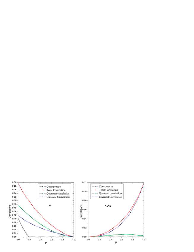
Figure 1: Correlation dynamics for the partitions $AB$ and $E_{A}E_{B}$ under action of the amplitude and phase damping reservoirs when the initial state is the Werner state ($a=0.4$). The lines with red triangle, flipped green triangle, blue star and black square represent total correlation, quantum correlation, classical correlation and entanglement, respectively.

In Fig. 1, various correlations are plotted as a function of the parameter $p$ for the bi-partitions $AB$ and $E_{A}E_{B}$ when the initial state is the Werner state with $a=0.4$. One can see that entanglement appears the sudden death (ESD) behavior ESD . Contrary to what happens to entanglement, the quantum correlation of $AB$ has no sudden death but monotonously decreases to zero in the asymptotic limit ($p=1$). It means the robustness of the quantum correlation to decoherence Markovian ; non-Markovian1 .

Although the classical correlation between qubits A and B decreases monotonously as $p$ increases, the classical correlation between $E_{A}$ and$\ E_{B}$ increases monotonously and arrives at the maximal value in the asymptotic limit ($p=1$). In this sense, one may say that the classical correlation lost from the partition $AB$ partially transfers to the partition $E_{A}E_{B}$.

However, much different from the quantum correlation between A and B, the quantum correlation of the partition $E_{A}E_{B}$ firstly increases and finally decreases to zero in the asymptotic limit, and shows the sudden change behavior during the evolution analytical . From Fig. 1, we also see that there is no entanglement between $E_{A}$ and$\ E_{B}$ in the whole $p$ range. Therefore, in contrast to the classical correlation, the entanglement and the quantum correlation for the partition $AB$ are not transferred to the two environments. This result is much different from that obtained only with amplitude-damping channels Main Ref and that presented in the reference PRL .

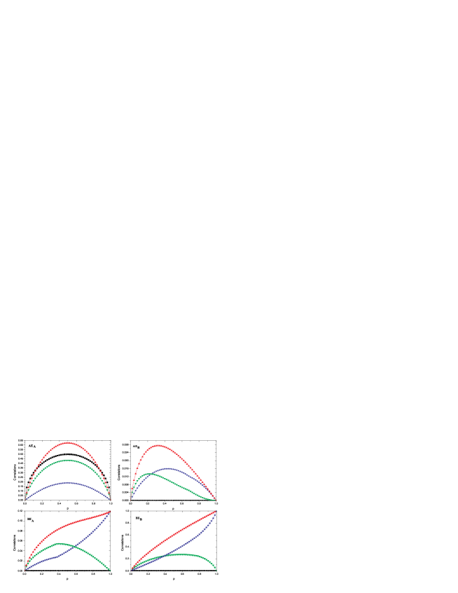
Figure 2: Correlation dynamics for the partitions $AE_{A},AE_{B},BE_{A}$ and $BE_{B}$ under the action of amplitude and phase damping environments when the initial state is the Werner state ($a=0.4$). The lines are marked as in Fig. 1.

The correlation dynamics for other bi-partitions, i.e., $AE_{A},AE_{B},BE_{A}$ and $BE_{B}$, are shown in Fig. 2. In these figures we see that the correlation dynamics between $A$ and the environments differs from that between $B$ and the environments. All the correlations (classical and quantum correlations) between $A$ and the environments completely vanish in the asymptotic limit. However, the classical correlation can be created between $B$ and $E_{A}$ ($E_{B}$). This result differs from the situation only with the amplitude-damping environments, where qubit can only construct nonclassical correlation with its own environment Main Ref . Another interesting result shown in Fig. 2 is that both the classical and quantum correlations of $BE_{A}$ exhibit sudden change behavior analytical . Fig. 2 also shows that during the evolution, the quantum correlation can be constructed in all the bi-partitions, but entanglement can only be created in $AE_{A}$.

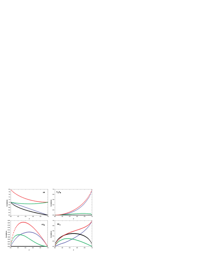
Figure 3: Correlation dynamics for the partitions $AB,E_{A}E_{B},AE_{B}$ and $BE_{A}$ with the amplitude damping and phase damping environments when the initial state is the Bell state ($a=1$). The lines are marked as in Fig. 1.

The correlation dynamics for the initial Bell state ($a=1$) is plotted in Fig. 3. It is very interesting that in the asymptotic limit the quantum correlation of $AB$ always remains and is equal to its initial value $1$ while the entanglement and the classical correlation decay to zero. This result completely differs from that of the Werner state as shown in Fig. 2. It shows that the nonclassical correlation can exist even in a separable state Ollivier . We also observe that the classical correlation transfers to the partitions $E_{A}E_{B}$ and $BE_{A}$.

III.2 Combining Amplitude-Damping and Bit-Flip Environments

Now let us consider the correlation dynamics for various bi-partitions of the system under the action of the amplitude-damping and flip reservoirs. Suppose that the qubits $A$ and $B$ are coupled to the amplitude-damping and bit-flip environments. The effect of a flip environment over qubit $B$ can be described by the state map map1 ; map2

$$\left|0\right\rangle_{B}\left|0\right\rangle_{E_{B}}\rightarrow\sqrt{p}\left|0\right\rangle_{B}\left|0\right\rangle_{E_{B}}+(i)^{k}\sqrt{q}\left|1\right\rangle_{B}\left|1\right\rangle_{E_{B}},$$ (25)

$$\left|1\right\rangle_{B}\left|0\right\rangle_{E_{B}}\rightarrow\sqrt{p}\left|1\right\rangle_{B}\left|0\right\rangle_{E_{B}}+(-i)^{k}\sqrt{q}\left|0\right\rangle_{B}\left|1\right\rangle_{E_{B}},$$ (26)

where $k=0$ is for the bit-flip environment, $k=1$ for the bit-phase-flip environment. Since the correlation dynamics does not depend on $k$, in what follows, we will consider only the bit-flip environment ($k=0$). The Kraus operators of the bit-flip are as follows Nielsen

$$\Gamma_{1}^{B}=\left(\begin{array}[]{cc}\sqrt{p}&0\\ 0&\sqrt{p}\end{array}\right),\Gamma_{2}^{B}=\left(\begin{array}[]{cc}0&\sqrt{q}\\ \sqrt{q}&0\end{array}\right).$$ (27)

The initial state of the whole system is still supposed to be (17). From Eqs. (11), (12), (25) and (26), we can obtain the density matrix of the whole system. The reduced density matrices for various bi-partitions can then be analytical obtained, which are given in the appendix A.

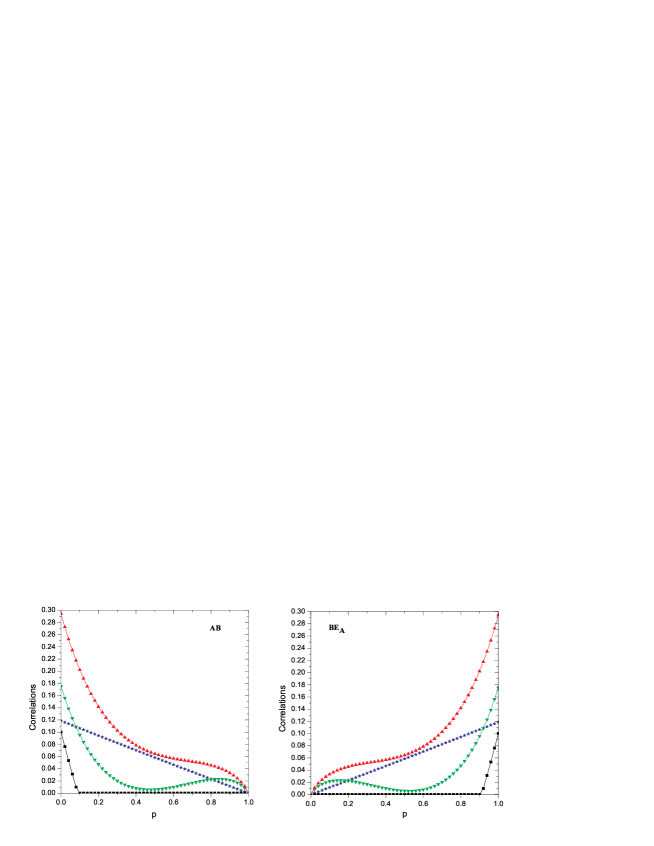
Figure 4: Correlation dynamics for the partitions $AB$ and $BE_{A}$ with the combined amplitude damping and bit flip environments when the initial state is the Werner state ($a=0.4$). The lines are marked as in Fig. 1.

In Fig. 4, the correlation dynamics for the bipartitions $AB$ and $BE_{A}$ are shown. We observe that the total, classical and quantum correlations vanish at the asymptotic limit $p=1$ but the entanglement suddenly and completely disappears at a finite point. It is also noticed that in the asymptotic limit all the correlations including entanglement are fully transferred to the partition $BE_{A}$ rather than that of the two environments $E_{A}$ and $E_{B}$ PRL ; Main Ref . In Fig. 5, the correlation dynamics for the other four bi-partitions are shown. From these figures, one may see that although there exist bipartite correlations during the evolution process, they all vanish in the asymptotic limit. The four bi-partitions $AE_{A},AE_{B},BE_{B}$ and $E_{B}E_{A}$ can then be treated as transfer bridges for correlations.

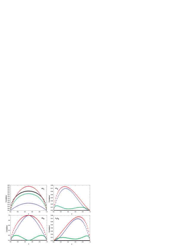
Figure 5: Correlation dynamics for the partitions $AE_{A},AE_{B},BE_{B}$ and $E_{A}E_{B}$ with the combined amplitude damping and bit fip environments when the initial state is the Werner state ($a=0.4$). The lines are marked as in Fig. 1.

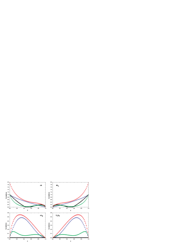
Figure 6: Correlation dynamics for the partitions $AB,E_{A}E_{B},AE_{B}$ and $BE_{A}$ with the combined amplitude damping and bit flip environments when the initial state is the Bell state ($a=1$). The lines are marked as in Fig. 1.

In Fig. 6, the correlation dynamics for various partitions of the system with the initial Bell state is shown. It is noticed that all the correlations and entanglement of $AB$ can be fully transferred to the partition $BE_{A}$. One may also find that there is the death and revival of entanglement under the action of the combined amplitude-damping and bit-flip environments for the Bell state with $a=1$.

From the above discussions, we obtain a very interesting result that all the quantum and classical correlations, and even the entanglement, originally prepared between the qubits $A$ and $B$, can be completely transferred to the partition $BE_{A}$ under the action of the amplitude damping and bit-flip environments.

III.3 Combining Phase-Damping and Phase-Flip Environments

In this subsection, we will consider the situation where two quits $A$ and $B$ interact independently and locally with the phase-damping and phase-flip environments, respectively. The corresponding state map induced by a phase-flip environment over qubit $B$ is given by map1 ; map2

$$\left|0\right\rangle_{B}\left|0\right\rangle_{E_{B}}\rightarrow\sqrt{p}\left|0\right\rangle_{B}\left|0\right\rangle_{E_{B}}+\sqrt{q}\left|0\right\rangle_{B}\left|1\right\rangle_{E_{B}},$$ (28)

$$\left|1\right\rangle_{B}\left|0\right\rangle_{E_{B}}\rightarrow\sqrt{p}\left|1\right\rangle_{B}\left|0\right\rangle_{E_{B}}-\sqrt{q}\left|1\right\rangle_{B}\left|1\right\rangle_{E_{B}}.$$ (29)

The Kraus operators of the phase-flip environment are as follows Nielsen

$$\Gamma_{1}^{B}=\left(\begin{array}[]{cc}\sqrt{p_{1}}&0\\ 0&\sqrt{p_{1}}\end{array}\right),\Gamma_{2}^{B}=\left(\begin{array}[]{cc}\sqrt{q_{1}}&0\\ 0&-\sqrt{q_{1}}\end{array}\right).$$ (30)

It is known that a unitary recombination of the elements in (16) can give the expression of (30) Nielsen . In particular, the phase-damping process is exactly the same as the phase-flip one when $p_{1}=(1+\sqrt{1-q})/2$. In the present investigation, we set $p_{1}=p$ and $q_{1}=1-p_{1}$ which guarantees that $A$ and $B$ undergoing non-identical environments.

Starting from the initial state defined by Eq. (17) and using the same method mentioned in the preceding subsections, we can obtain the reduced density matrices for various bi-partitions of the system, which are shown in the appendix B.

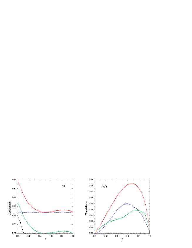
Figure 7: Correlation dynamics for the partitions $AB$ and $E_{A}E_{B}$ with the combined phase damping and phase flip environments when the initial state is the Werner state ($a=0.4$). The lines are marked as in Fig. 1.

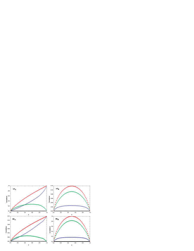
Figure 8: Correlation dynamics for the partitions $AE_{A},AE_{B},BE_{A}$ and $BE_{B}$ with the combined phase damping and phase flip environments for the Werner state ($a=0.4$). The lines are marked as in Fig. 1.

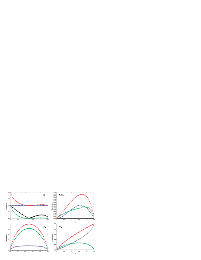
Figure 9: Correlation dynamics for the partitions $AB,E_{A}E_{B},AE_{B}$ and $BE_{A}$ with the combined phase damping and phase flip environments for the Bell state ($a=1$). The lines are marked as in Fig. 1.

In Fig. 7, the correlation dynamics for the partitions $AB$ and $E_{A}E_{B}$ is shown. It can be seen that the total and quantum correlations display the decay and revival behavior while the entanglement exhibits the ESD. This result differs from that of the pure phase-damping environment where the quantum and total correlations monotonously decrease with $p$ increasing Main Ref . In particular, the classical correlation of $AB$ remains a constant in the whole range. This indicates that the classical correlation is immune to the decoherence. This result may lead to an operational way of measuring both the classical and quantum correlation in a composite system analytical . All the correlations of $E_{A}E_{B}$ firstly increase and reach to the maximal values with $p$ increasing, and then decrease to zero in the asymptotic limit ($p=1$). This phenomenon differs also from that of the pure phase-damping environment where classical and quantum correlations between the environments reach to a same finite value at $p=1$ Main Ref .

Fig. 8 shows the correlation evolution for other bi-partitions of the system. It is observed that only the classical correlations can be created among the bi-partitions $AE_{A}$ and $BE_{A}$ in the asymptotic limit ($p=1$). The quantum correlation can exist among the various bi-partitions only during the evolution. However, there exist no entanglement between any partitions during the whole evolution and the entanglement exiting in the initial state is fully evaporated, which is very similar to that of the pure phase-damping noisy environment Main Ref .

The correlation dynamics is shown in Fig. 9 when the two qubits are initially in the Bell state . In these figures, it is seen that the entanglement displays the death and revival phenomenon and the classical correlation keeps constant during the evolution. The quantum correlation and entanglement existing in the initial state are fully evaporated in the asymptotic limit ($p=1$). As the same as shown in Fig. 8, only the classical correlation between the qubit $A(B)$ and the phase-damping environment can be created.

IV Summary

We study the quantum and classical correlation (including entanglement) dynamics of two qubits $A$ and $B$ which are independently and locally coupled to two non-identical environments $E_{A}$ and $E_{B}$, respectively. Three different combinations of noisy environments are considered, i.e., the amplitude plus phase damping environments (APE), the amplitude-damping plus the bit-flip environments (ABE) and the phase-damping plus the phase-flip environments (PPE). We find that, contrary to the single-type noisy environment case, the entanglement and quantum correlation transfer direction can be controlled by combining the different noisy environments. This may provides us a way of manipulating the correlation dynamics of a composite system. The amplitude-damping environment plays a very important role in the correlation dynamics. It determines whether there exists a correlation transfer among the bi-partitions of a composite system. If there is no amplitude damping, e.g. in the PPE, the initial entanglement is completely evaporated. In the ABE case we show that all the quantum and classical correlations, and even entanglement, which exist in the initial state of the two qubits, can be completely transferred to the bi-partition $BE_{A}$ without any loss. When the initial state is the Bell one, in the APE case the quantum correlation between the two qubits can remain the initial value in the asymptotic limit while the classical correlation and entanglement decay to zero, but in the PPE case the classical correlation keeps constant while the quantum correlation and entanglement decay to zero. This result shows that it is possible to distinguish the quantum correlation form the classical correlation and entanglement by combining different kinds of environments. In the combined environments ABE and PPE, even for the Bell state, the entanglement can display the sudden death (ESD) and revival phenomenon. We also notice that the quantum correlation can appear in arbitrary bi-partitions and have no sudden death behavior during the evolution, which means the robustness of the quantum correlation to decoherence.

IV.1 Appendix A: Reduced Density Matrices for Various Bi-partitions under the Action of Amplitude-Damping and Bit-Flip Environments

The reduced density matrix for the partition $AB$, obtained by taking the partial trace of $\rho_{ABE_{A}E_{B}}$ over the degrees of freedom of the reservoir is given by

$$\rho_{AB}=\frac{1}{4}\left(\begin{array}[]{cccc}2p^{2}+qa_{-}&0&0&\sqrt{q}(pb_{-}+qb_{+})\\ 0&2p^{2}+qa_{+}&\sqrt{q}(pb_{+}+qb_{-})&0\\ 0&\sqrt{q}(pb_{+}+qb_{-})&q(pa_{-}+qa_{+})&0\\ \sqrt{q}(pb_{-}+qb_{+})&0&0&q(qa_{-}+pa_{+})\end{array}\right).$$ (31)

For the partitions $AE_{A},BE_{B},AE_{B}$ and $BE_{A}$, the reduced-density operators are as follows

$$\rho_{AE_{A}}=\frac{1}{2}\left(\begin{array}[]{cccc}1&0&0&0\\ 0&p&\sqrt{pq}&0\\ 0&\sqrt{pq}&q&0\\ 0&0&0&0\end{array}\right),$$ (32)

$$\rho_{BE_{B}}=\frac{1}{2}\left(\begin{array}[]{cccc}p&0&0&\sqrt{pq}\\ 0&q&\sqrt{pq}&0\\ 0&\sqrt{pq}&p&0\\ \sqrt{pq}&0&0&q\end{array}\right),$$ (33)

$$\rho_{AE_{B}}=\frac{1}{2}\left(\begin{array}[]{cccc}(p+p^{2})&0&0&q\sqrt{p}c_{1}\\ 0&(1+p)q&q\sqrt{p}c_{1}&0\\ 0&q\sqrt{p}c_{1}&pq&0\\ q\sqrt{p}c_{1}&0&0&q^{2}\end{array}\right),$$ (34)

$$\rho_{BE_{A}}=\frac{1}{4}\left(\begin{array}[]{cccc}(1+p)D&0&0&\sqrt{p}B\\ 0&pC&\sqrt{p}A&0\\ 0&\sqrt{p}A&(1+p)C&0\\ \sqrt{p}B&0&0&pD\end{array}\right),$$ (35)

where $A=(qb_{-}+pb_{+}),B=(pb_{-}+qb_{+}),C=(pa_{-}+qa_{+})$ and $D=(pa_{+}+qa_{-})$.

After tracing out the degrees of freedom of the two qubits, we obtain the reduced density matrix for the two environments $E_{A}$ and $E_{B}$

$$\rho_{E_{A}E_{B}}=\frac{1}{2}\left(\begin{array}[]{cccc}p(1+q)&0&0&p\sqrt{q}c_{1}\\ 0&q(2-p)&p\sqrt{q}c_{1}&0\\ 0&p\sqrt{q}c_{1}&p^{2}&0\\ p\sqrt{q}c_{1}&0&0&pq\end{array}\right).$$ (36)

IV.2 Appendix B: Density Matrices for Various Bi-partitions under the Action of Phase-Damping and Phase-Flip Environments

The reduced density matrix for $AB$ under the influence of the mixed phase damping and phase flip environments is

$$\rho_{AB}=\frac{1}{4}\left(\begin{array}[]{cccc}a_{+}&0&0&\sqrt{q}(p-q)b_{-}\\ 0&a_{-}&\sqrt{q}(p-q)b_{+}&0\\ 0&\sqrt{q}(p-q)b_{+}&a_{-}&0\\ \sqrt{q}(p-q)b_{-}&0&0&a_{+}\end{array}\right).$$ (37)

For the partitions $AE_{A},BE_{B},AE_{B}$ and $BE_{A}$, the reduced-density operators are analytically given by

$$\rho_{AE_{A}}=\frac{1}{2}\left(\begin{array}[]{cccc}1&0&0&0\\ 0&0&0&0\\ 0&0&q&\sqrt{pq}\\ 0&0&\sqrt{pq}&p\end{array}\right),$$ (38)

$$\rho_{BE_{B}}=\frac{1}{2}\left(\begin{array}[]{cccc}p&\sqrt{pq}&0&0\\ \sqrt{pq}&q&0&0\\ 0&0&p&-\sqrt{pq}\\ 0&0&-\sqrt{pq}&q\end{array}\right),$$ (39)

$$\rho_{AE_{B}}=\frac{1}{2}\left(\begin{array}[]{cccc}p&\sqrt{pq}c_{3}&0&0\\ \sqrt{pq}c_{3}&q&0&0\\ 0&0&p&-\sqrt{pq}c_{3}\\ 0&0&-\sqrt{pq}c_{3}&q\end{array}\right),$$ (40)

$$\rho_{BE_{A}}=\frac{1}{4}\left(\begin{array}[]{cccc}a_{+}+qa_{-}&0&\sqrt{pq}a_{-}&0\\ 0&a_{-}+qa_{+}&0&\sqrt{pq}a_{+}\\ \sqrt{pq}a_{-}&0&pa_{-}&0\\ 0&\sqrt{pq}a_{+}&0&pa_{+}\end{array}\right).$$ (41)

Similarly, the reduced density matrix for partition $E_{A}E_{B}$ is

$$\rho_{E_{A}E_{B}}=\frac{1}{2}\left(\begin{array}[]{cccc}p(1+q)&-p\sqrt{pq}c_{3}&p\sqrt{pq}&-pqc_{3}\\ -p\sqrt{pq}c_{3}&q(1+q)&-pqc_{3}&q\sqrt{pq}\\ p\sqrt{pq}&-pqc_{3}&p^{2}&-p\sqrt{pq}c_{3}\\ -pqc_{3}&q\sqrt{pq}&-p\sqrt{pq}c_{3}&pq\end{array}\right).$$ (42)

References

- (1) M. A. Neilsen and I. L. Chuang, Quantum Computation and Quantum Information (Cambridge University Press, Cambridge, England, 2000).
- (2) H. Ollivier and W. H. Zurek, Phys. Rev. Lett. 88, 017901 (2001).
- (3) L. Henderson and V. Vedral, J. Phys. A 34, 68899 (2001).
- (4) V. Vedral, Phys. Rev. Lett. 90, 050401 (2003).
- (5) B. P. Lanyon, M. Barbieri, M. P. Almeida, and A. G. White, Phys. Rev. Lett. 101, 200501 (2008).
- (6) E. Knill and R. Laflamme, Phys. Rev. Lett. 81, 5672 (1992).
- (7) J. Oppenheim, M. Horodecki, P. Horodecki, and R. Horodecki, Phys. Rev. Lett. 89, 180402 (2002).
- (8) B. Groisman, S. Popescu, and A. Winter, Phys. Rev. A 72, 032317 (2005).
- (9) S. Luo, Phys. Rev. A 77, 022301 (2008).
- (10) K. Modi, T. Paterek, W. Son, V. Vedral, and M. Williamson, Phys. Rev. Lett. 104, 080501 (2010).
- (11) J. Maziero, L. C. Céleri, R. M. Serra, and V. Vedral, Phys. Rev. A 80, 044102 (2009).
- (12) Mazhar Ali, A. R. P. Rau, G. Alber, Phys. Rev. A 81, 042105 (2010).
- (13) R. Dillenschneider, Phys. Rev. B 78, 224413 (2008).
- (14) M. S. Sarandy, Phys. Rev. A 80, 022108 (2009).
- (15) T. Werlang, G. Rigolin, Phys. Rev. A 81, 044101 (2010).
- (16) T. Werlang, C. Trippe, G. A. P. Ribeiro, G. Rigolin, Phys. Rev. Lett. 105, 095702 (2010).
- (17) Z. -Y Sun, L. Li, K. -L Yao, G. -H Du, J. -W Liu, B. Luo, N. Li and H. -N Li, Phys. Rev. A 82, 032310 (2010).
- (18) P. Giorda, M. G. A. Paris, Phys. Rev. Lett. 105, 020503 (2010).
- (19) G. Adesso, A. Datta, Phys. Rev. Lett. 105, 030501 (2010).
- (20) T. Werlang, S. Souza, F. F. Fanchini, and C. J. Villas Boas, Phys. Rev. A 80, 024103 (2009).
- (21) F. F. Fanchini, T. Werlang, C. A. Brasil, L. G. E. Arruda, and A. O. Caldeira, Phys. Rev. A 81, 052107 (2010).
- (22) L. Mazzola, J. Piilo, and S. Maniscalco, arXiv:1006.1805 (2010).
- (23) L. Mazzola, J. Piilo, and S. Maniscalco, Phys. Rev. Lett. 104, 200401 (2010).
- (24) L. C. Céleri, A. G. S. Landulfo, R. M. Serra, and G. E. A. Matsas, Phys. Rev. A 81, 062130 (2010).
- (25) F. F. Fanchini, L. K. Castelano, A. O. Caldeira, arXiv:0912.1468 (2010).
- (26) J. Maziero, T. Werlang, F. F. Fanchini, L. C. Céleri, R. M. Serra, Phys. Rev. A 81, 022116 (2010).
- (27) J. -S. Xu, X. -Y. Xu, C. -F. Li, C. -J. Zhang, X. -B. Zou, and G. -C. Guo, Nat. Commun. 1, 7 (2010).
- (28) J. -S. Xu, C. -F. Li, C. -J. Zhang, X. -Y. Xu, Y. -S. Zhang, and G. -C. Guo, arXiv:1005.4510 (2010).
- (29) D. O. Soares-Pinto, L. C. Céleri, R. Auccaise, F. F. Fanchini, et al., Phys. Rev. A 81, 062118 (2010).
- (30) C. E. López, G. Romero, F. Lastra, E. Solano, and J. C. Retamal, Phys. Rev. Lett. 101, 080503 (2008).
- (31) B. Groisman, S. Popescu, and A. Winter, Phys. Rev. A 72, 032317 (2005).
- (32) B. Schumacher, M. D. Westmoreland, Phys. Rev. A 74, 042305 (2006).
- (33) B. M. Terhal, M. Horodecki, D. W. Leung, and D. P. DiVincenzo, J. Math. Phys. 43, 4286 (2002).
- (34) D. P. DiVincenzo, M. Horodecki, D. W. Leung, J. A. Smolin, and B. M. Terhal, Phys. Rev. Lett. 92, 067902 (2004).
- (35) M. Piani, P. Horodecki, and R. Horodecki, Phys. Rev. Lett. 100, 090502 (2008).
- (36) M. Piani, M. Christandl, C. E. Mora, and P. Horodecki, Phys. Rev. Lett. 102, 250503 (2009).
- (37) D. W. Leung, J. Math. Phys. 44, 528 (2003).
- (38) A. Salles, F. de Melo, M. P. Almeida, M. Hor-Meyll, S. P. Walborn, P. H. Souto Ribeiro, and L. Davidovich, Phys. Rev. A 78, 022322 (2008).
- (39) W. K. Wootters, Phys. Rev. Lett. 80, 2245 (1998).
- (40) T. Yu, J. H. Eberly, Phys. Rev. Lett. 93, 140404 (2004); T. Yu, J. H. Eberly, ibid. 96, 140403 (2006); T. Yu, J. H. Eberly, Science 323, 598 (2009).