Error Estimates in Horocycle Averages Asymptotics:
Challenges from String Theory

Abstract.

There is an intriguing connection between the dynamics of the horocycle flow in the modular surface $SL_{2}(\boldsymbol{Z})\backslash SL_{2}(\boldsymbol{R})$ and the Riemann hypothesis. It appears in the error term for the asymptotic of the horocycle average of a modular function of rapid decay. We study whether similar results occur for a broader class of modular functions, including functions of polynomial growth, and of exponential growth at the cusp. Hints on their long horocycle average are derived by translating the horocycle flow dynamical problem in string theory language. Results are then proved by designing an unfolding trick involving a Theta series, related to the spectral Eisenstein series by Mellin integral transform. We discuss how the string theory point of view leads to an interesting open question, regarding the behavior of long horocycle averages of a certain class of automorphic forms of exponential growth at the cusp.

1. Introduction

In this paper we exploit a novel angle for obtaining some insights on the long horocycle average asymptotic for certain classes of $SL_{2}(\boldsymbol{Z})$-invariant automorphic functions. We focus on modular functions of polynomial growth at the cusp, and on a certain class of modular functions of (bounded) exponential growth. Automorphic functions with such growing conditions play a role in string theory, in the context of perturbative (one-loop) closed string amplitudes. Remarkably, their horocycle averages contain information on the numbers of physical degrees of freedom of closed strings particle-like excitations [C1],[CC1],[CC3],[ACER].

The advantage of translating the dynamical problem in string theory language is in the possibility of using consistency conditions from string theory to gain insights on the horocycle average asymptotic. For the two classes of modular forms we focus on, the string theory perspective suggests a universal behavior of their long horocycle average, which appears somehow surprising from the perspective of the theory of automorphic forms. Our results are then obtained by an unfolding method that involves a Theta series, connected to the spectral Eisenstein series by Mellin integral transform. We illustrate advantages of the Theta unfolding for dealing with automorphic forms of not so mild growing conditions, over the classical Rankin-Selberg method. In particular, we derive some results previously obtained by Zagier [Za2] via considerably shorter proofs on the analytic continuation of the Rankin-Selberg integral transform for automorphic functions of polynomial growth. We then obtain asymptotics for long horocycle averages of modular functions of polynomial growth, including a relation between the error estimate and the Riemann hypothesis. For modular function of rapid decay the same kind of relation was originally obtained in [Za1].

When applied to modular functions playing a role in string theory, our results lead to fascinating connections between enumerative properties of closed string spectra and the Riemann hypothesis [C1],[CC1],[ACER],[CC2],[CC3]. These connections extend to multi-loops closed string amplitudes [CC1],[CC3] and results for measure rigidity of unipotent flows in homogenous spaces [Ra] are intertwined with properties of perturbative closed string theory [CC2].

Let $\boldsymbol{\mathcal{H}}=\{z=x+iy\in\boldsymbol{\mathbb{C}}|y>0\}$ be the upper complex plane, horocycles in $\boldsymbol{\mathcal{H}}$ are both circles tangent to the real axis in rational points (cusps), and horizonal lines, (which can be thought as circles tangent to the $z=i\infty$ cusp).

$\begin{pmatrix}a&b\\ c&d\end{pmatrix}\in SL_{2}(\boldsymbol{R})$ acts on $z\in\boldsymbol{\mathcal{H}}$ through the Möbius transformation $z\rightarrow\frac{az+b}{cz+d}$. The following one-parameter action of the upper triangular unipotent subgroup $\boldsymbol{U}\subset SL_{2}(\boldsymbol{R})$

$$\boldsymbol{g}_{u}:=\Big{\{}\begin{pmatrix}1&t\\ 0&1\end{pmatrix},\,|t|\leq|u|,\,\Big{\}},\qquad u\in\mathbb{R}$$

generates motions along horizontal lines in $\boldsymbol{\mathcal{H}}$. Long horocycles in $\boldsymbol{\mathcal{H}}$ do not exhibit interesting dynamics in the half-plane $\boldsymbol{\mathcal{H}}$, since the orbit $\boldsymbol{g}_{u}(x+iy)=\{x+t+iy,|t|\leq|u|\}$ for $u\rightarrow\pm\infty$ just escapes to infinity. However, $\boldsymbol{g}_{u}(x+iy)$ has an interesting dynamics in the quotient space $\boldsymbol{\Gamma}\backslash\boldsymbol{\mathcal{H}}$, $\boldsymbol{\Gamma}\simeq SL_{2}(\boldsymbol{Z})$. The horocycle $\boldsymbol{g}_{u=1}(x+iy)$ is a closed orbit in $\boldsymbol{\Gamma}\backslash\boldsymbol{\mathcal{H}}$ with length $1/y$, as measured by the hyperbolic metric $ds^{2}=y^{-2}(dx^{2}+dy^{2})$. Quite remarkably, in the long length limit $y\rightarrow 0$, the horocycle $\boldsymbol{g}_{u=1}(x+iy)$ tends to cover uniformly the modular domain $\boldsymbol{\Gamma}\backslash\boldsymbol{\mathcal{H}}$ [He], [Fu],[DS], (see figure 1. for plots of horocycles in the modular domain of increasing length obtained with Mathematica)

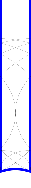
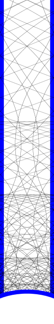
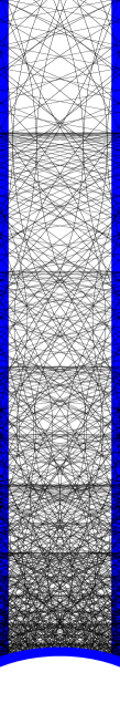
Figure 1. Modular images of horocycles of increasing length. It is interesting to study the image of $H_{\alpha}=\mathbb{R}+i\alpha$ in the standard $SL_{2}(\boldsymbol{Z})$ fundamental domain as $\alpha\rightarrow 0$. Left: modular image of the line $y=\frac{1}{8}$. Center: modular image of the line $y=\frac{1}{100}$. Right: modular image of the line $y=\frac{1}{400}$. In all cases the modular domain is truncated at $y>10$. The modular image of a line $y=\alpha$ tends to become dense for $\alpha\rightarrow 0$ [He].

Methods involving the theory of automorphic forms lead to interesting results for horocycle flow asymptotic. Quite remarkable is the relation between error estimates for asymptotics involving the average of an automorphic forms along long horocycles and the Riemann hypothesis. By using the Rankin-Selberg method, Zagier [Za1] has obtained the intriguing result

(1.1) $$\int_{0}^{1}dxf(x,y)\sim\frac{3}{\pi}\int_{\boldsymbol{\mathcal{D}}}d\mu f+O(y^{1-\frac{\Theta}{2}}),\qquad y\rightarrow 0$$

when $f$ is a smooth modular invariant function of rapid decay at the cusp $y\rightarrow\infty$. Indeed, in order to have a sufficient condition for (1.1) to hold, one has to add some smoothness condition on $f$ and a growing condition on its Laplacian $\Delta f$, [Ve], (this is discussed in details in §2, proposition 3). In eq. (1.1) $\mu$ is the hyperbolic $\boldsymbol{\mathcal{H}}$ measure, $d\mu=y^{-2}dxdy$, and the error estimate is governed by $\Theta=\rm{Sup}\{\Re(\rho)|\boldsymbol{\zeta}^{*}(\rho)=0\}$, the superior of the real part of the non trivial zeros of the Riemann zeta function $\boldsymbol{\zeta}(s)$, ($\boldsymbol{\zeta}^{*}(s)=\pi^{-s/2}\boldsymbol{\Gamma}(s/2)\boldsymbol{\zeta}(s)$).

The error estimate for the convergence rate in (1.1) is remarkably linked to the Riemann hypothesis (RH), indeed, RH is equivalent to the following condition

(1.2) $$\int_{0}^{1}dxf(x,y)\sim\frac{3}{\pi}\int_{\boldsymbol{\mathcal{D}}}d\mu f+O(y^{3/4-\epsilon}),\qquad y\rightarrow 0$$

for every $f\in C_{00}^{\infty}(\boldsymbol{\Gamma}\backslash\mathcal{H})$. Up to date, the error term is $o(y^{1/2})$ unconditionally as a consequence of the bound $\Theta\leq 1$ on the real part of the Riemann zeta functions zeros $\rho$’s.

Notation and Terminology

$\bullet$ $\boldsymbol{\mathcal{H}}=\{z=x+iy\in\mathbb{C},\,\,y>0\}$, the upper complex plane.

$\bullet$ $\boldsymbol{\Gamma}\simeq SL_{2}(\boldsymbol{Z})$, the modular group.

$\bullet$ $\boldsymbol{\mathcal{D}}\simeq\boldsymbol{\Gamma}\backslash\boldsymbol{\mathcal{H}}$, the standard $SL_{2}(\boldsymbol{Z})$ fundamental domain with cusp at $z=i\infty$

$\bullet$ $\boldsymbol{\Gamma}_{\infty}\subset\boldsymbol{\Gamma}$, the subgroup of upper triangular matrices.

$\bullet$ $\boldsymbol{\zeta}(s)=\sum_{n\in\mathbb{N}}n^{-s}$, $\Re(s)>1$, the Riemann zeta function.

$\bullet$ $\boldsymbol{\zeta}^{*}(s)=\pi^{-s/2}\boldsymbol{\Gamma}(s/2)\boldsymbol{\zeta}(s)$.

$\bullet$ $\boldsymbol{\Theta}_{t}(z)=\sum_{(m,n)\in\mathbb{Z}^{2}\backslash\{0\}}e^{-\pi t\frac{|mz+n|^{2}}{y}}$.

$\bullet$ $\boldsymbol{E}_{s}(z)=\frac{1}{2}\sum_{(c,d)\in\mathbb{Z}^{2},(c,d)=1}y^{s}|cz+d|^{-2s}$.

$\bullet$ $\boldsymbol{E}^{*}_{s}(z)=\pi^{-s}\boldsymbol{\Gamma}(s)\sum_{(m,n)\in\mathbb{Z}^{2}\backslash\{0\}}y^{s}|mz+n|^{-2s}$.

$\bullet$ $\boldsymbol{\vartheta}_{t}(y)=\sum_{n\in\mathbb{N}_{>0}}e^{-\pi\frac{t}{y}n^{2}}$.

$\bullet$ $\boldsymbol{\mathcal{M}}_{y}[\varphi](s)=\int_{0}^{\infty}dyy^{s-1}\varphi(y)$, the Mellin transform of the function $\varphi$.

$\bullet$ $\mathcal{P}[\varphi](z)=\sum_{\gamma\in\boldsymbol{\Gamma}_{\infty}\backslash\boldsymbol{\Gamma}}\varphi(\Im(\gamma(z)))$, the Poincaré series of the function $\varphi:\mathbb{R}_{>0}\rightarrow\mathbb{C}$.

$\bullet$ $\boldsymbol{a}_{0}(y)=\int_{0}^{1}dxf(x,y)$, the constant term of the modular invariant function $f(x,y)=\sum_{n\in\mathbb{Z}}\boldsymbol{a}_{n}(y)e^{2\pi inx}$.

$\bullet$ $\langle f,g\rangle_{\boldsymbol{\Gamma}\backslash\boldsymbol{\mathcal{H}}}=\int_{\boldsymbol{\mathcal{D}}}dxdyy^{-2}\bar{f}(z)g(z)$, the Petersson inner product of the modular invariant functions $f(z)$, $g(z)$.

$\bullet$ $\langle\varphi,\xi\rangle_{\boldsymbol{U}\backslash\boldsymbol{\mathcal{H}}}=\int_{0}^{\infty}dyy^{-2}\bar{\varphi}(y)\xi(y)$, the inner product on the space of functions $\boldsymbol{U}\backslash\boldsymbol{\mathcal{H}}\simeq\mathbb{R}_{>0}\rightarrow\mathbb{C}$.

Due to $\boldsymbol{\Gamma}_{\infty}=\boldsymbol{U}\cap SL_{2}(\boldsymbol{Z})$ invariance, a modular invariant function $f=f(x,y)$, can be decomposed in Fourier series in the $x$ variable, $f(x,y)=\sum_{n\in\mathbb{Z}}\boldsymbol{a}_{n}(y)e^{2\pi inx}$. The constant Fourier term $\boldsymbol{a}_{0}(y)$ then gives the $f$ average along the horocycle $\boldsymbol{\mathcal{H}}_{y}:=(\mathbb{R}+iy)/\boldsymbol{\Gamma}_{\infty}$

(1.3) $$\boldsymbol{a}_{0}(y)=\int_{0}^{1}dxf(x,y)=\frac{1}{L(\boldsymbol{\mathcal{H}}_{y})}\int_{\boldsymbol{\mathcal{H}}_{y}}dsf,$$

where $L(\boldsymbol{\mathcal{H}}_{y})=1/y$ is the horocycle length, measured by the hyperbolic $\boldsymbol{\mathcal{H}}$ metric, $ds=y^{-1}\sqrt{dx^{2}+dy^{2}}$.

In this paper we focus on two classes of growing conditions for $SL_{2}(\boldsymbol{Z})$-invariant functions:

modular functions with polynomial growth at the cusp $y\rightarrow\infty$

(1.4) $$\boldsymbol{\mathcal{C}}_{TypeII}=\{f(x,y)\sim\sum_{i=1}^{l}\frac{c_{i}}{n_{i}!}\,y^{\alpha_{i}}\log^{n_{i}}y,\,\,y\rightarrow\infty,\,\,\,c_{i},\alpha_{i}\in\mathbb{C},\Re(\alpha_{i})<1/2,n_{i}\in\mathbb{N}_{\geq 0}\},$$

and modular functions with bounded exponential growth at the cusp, whose horocycle average $\boldsymbol{a}_{0}(y)$ grows polynomially at the cusp $y\rightarrow\infty$:

(1.5) $$\boldsymbol{\mathcal{C}}_{Heterotic}=\{f(x,y)\sim y^{\alpha}e^{\pi\beta y}e^{2\pi i\kappa x},y\rightarrow\infty;\beta<1,\kappa\in\mathbb{Z}\backslash\{0\},\Re(\alpha)<1/2\}.$$

The choices of symbols $\boldsymbol{\mathcal{C}}_{TypeII}$ and $\boldsymbol{\mathcal{C}}_{Heterotic}$, reflect the appearance of modular functions with such growing conditions respectively in type II string and heterotic string genus one closed string amplitudes, (with no tachyons in the spectrum). Bounds on $\alpha$ and on $\beta$ in (1.4) and (1.5) are universal in string theory, and follow by consistency requirements, (unitarity of the quantum worldsheet conformal field theory [GSW]).

String theory suggests that automorphic functions with growing conditions in $\boldsymbol{\mathcal{C}}_{TypeII}$ or in $\boldsymbol{\mathcal{C}}_{Heterotic}$ do have convergent horocycle average in the long limit $y\rightarrow 0$, and should exhibit asymptotic behavior similar to (1.1).

In this paper we prove theorems for long horocycle average asymptotic of automorphic functions in $\boldsymbol{\mathcal{C}}_{TypeII}$. We also prove some weaker results for $\boldsymbol{\mathcal{C}}_{Heterotic}$, and leave open the complete answer on long horocycle averages for automorhic functions in $\boldsymbol{\mathcal{C}}_{Heterotic}$. We believe this is an interesting open question, since peculiar features of the class of function $\boldsymbol{\mathcal{C}}_{Heterotic}$ and the bounds on $\alpha$ and on $\beta$ for a sufficient condition for convergence of the long horocycle average do not seem to emerge from the theory of automorphic functions. A complete answer on the horocycle average asymptotic for modular function in $\boldsymbol{\mathcal{C}}_{Heterotic}$ would probe the benefit one may actually gain by translating the homogenous dynamics horocycle problem in string theory terms.

In the rest of the introduction, we summarize our results and illustrate ideas and methods employed to derive them. In order to introduce main concepts on which we focus in this paper, we start in the next section with a brief illustration on how the asymptotic displayed in (1.1) for modular function of rapid decay is derived by the Rankin-Selberg method [Za1], (more material on that is presented in §2).

We then switch to modular functions of polynomial growth and discuss why their long horocycle asymptotic behavior cannot be derived by the standard Rankin-Selberg method. In dealing with modular functions of polynomial growth, Zagier [Za2] has designed a Rankin-Selberg method which is based on an unfolding method for modular integrals on a truncated version of the fundamental domain $\boldsymbol{\mathcal{D}}$. We contrast Zagier’s method with an alternative unfolding method we propose here, which relies on a unfolding trick employing the theta series $\boldsymbol{\Theta}_{t}(\tau)$. This theta series $\boldsymbol{\Theta}_{t}(\tau)$ is related to the spectral Eisenstein series $\boldsymbol{E}_{s}(\tau)$ by a Mellin transform. One of the advantages of this Theta method is to avoid complications with unfolding on a truncated version of the fundamental domain $\boldsymbol{\mathcal{D}}$.

1.1. Modular functions of rapid decay and the Rankin-Selberg method

Let us consider the Rankin-Selberg integral

(1.6) $$\langle\boldsymbol{E}_{s}(z),f(z)\rangle_{\boldsymbol{\Gamma}\backslash\boldsymbol{\mathcal{H}}}=\int_{\boldsymbol{\mathcal{D}}}dxdyy^{-2}\boldsymbol{E}_{s}(z)\,f(x,y),$$

when $f=f(x,y)$ is a modular invariant function of rapid decay at the cusp $y\rightarrow\infty$.

The spectral Eisenstein series $\boldsymbol{E}_{s}(z)$ has a Poincaré series representation for $\Re(s)>1$

(1.7) $$\boldsymbol{E}_{s}(z)=\sum_{\gamma\in\boldsymbol{\Gamma}_{\infty}\backslash\boldsymbol{\Gamma}}\Im(\gamma(z))^{s},\qquad\Re(s)>1,$$

where $\gamma(z)=\frac{az+b}{cz+d}$, with $\begin{pmatrix}a&b\\ c&d\end{pmatrix}\in\boldsymbol{\Gamma}$.

The possibility of exchanging the series with the integration on the fundamental domain $\boldsymbol{\mathcal{D}}$

$$\int_{\boldsymbol{\mathcal{D}}}dxdyy^{-2}\boldsymbol{E}_{s}(z)\,f(x,y) = \int_{\boldsymbol{\mathcal{D}}}dxdyy^{-2}\,f(x,y)\,\sum_{\boldsymbol{\gamma}\in\boldsymbol{\Gamma}_{\infty}\backslash\boldsymbol{\Gamma}}\Im(\gamma(z))^{s}$$

$$= \sum_{\gamma\in\boldsymbol{\Gamma}_{\infty}\backslash\boldsymbol{\Gamma}}\int_{\boldsymbol{\mathcal{D}}}dxdyy^{-2}\,f(x,y)\,\Im(\gamma(z))^{s},$$

(1.8)

amounts in being able to perform the unfolding trick. This corresponds to using modular transformations $\gamma\in\boldsymbol{\Gamma}_{\infty}\backslash\boldsymbol{\Gamma}$, to unfold the integration domain $\boldsymbol{\mathcal{D}}\simeq\boldsymbol{\Gamma}\backslash\boldsymbol{\mathcal{H}}$ into the half-infinite strip $\boldsymbol{\Gamma}_{\infty}\backslash\boldsymbol{\mathcal{H}}\simeq[-1/2,1/2)\times(0,\infty)\subset\boldsymbol{\mathcal{H}}$.

When $f=f(x,y)$ is of rapid decay at the cusp $y\rightarrow\infty$, since $\boldsymbol{E}_{s}(z)$ is of polynomial growth at the cusp

$$\boldsymbol{E}_{s}(z)\sim y^{s}+\frac{\boldsymbol{\zeta}^{*}(2s-1)}{\boldsymbol{\zeta}^{*}(2s)}y^{1-s}+o(y^{-N}),\qquad y\rightarrow\infty,\qquad\forall N>0,$$

eq. (1.8) follows by Lebesgue dominated convergence theorem on the sequence of products of partial sums of the series in (1.7) times the function $f(x,y)$.

This leads to connect the Rankin-Selberg integral to the Mellin transform of the function $\boldsymbol{a}_{0}(y)/y$

(1.9) $$\int_{0}^{\infty}dy\,y^{s-2}\boldsymbol{a}_{0}(y)=\int_{\boldsymbol{\mathcal{D}}}dxdy\,y^{-2}\boldsymbol{E}_{s}(z)f(x,y).$$

A relevant issue at this point is to determine analytic properties of the integral in the r.h.s. as a function of the complex variable $s$. Uniform convergence for $y\rightarrow\infty$ of the Rankin-Selberg integral with respect to the complex variable $s$, assures that the integral function in the r.h.s. $\boldsymbol{I}(s):=\langle\boldsymbol{E}_{s}(z),f(z)\rangle_{\boldsymbol{\Gamma}\backslash\boldsymbol{\mathcal{H}}}$ inherits analytic properties of $\boldsymbol{E}_{s}(z)$. In the present case $f$ is of rapid decay, and uniform convergence of the integral function $\boldsymbol{I}(s)$ holds. Thus the Mellin transform in the l.h.s. of (1.9) inherits as a function of the variable $s\in\mathbb{C}$ the same analytic properties of the Eisenstein series $\boldsymbol{E}_{s}(z)$.

The spectral Eisenstein series $\boldsymbol{E}_{s}(z)$ has a simple pole in $s=1$ with residue $\frac{1}{2\boldsymbol{\zeta}^{*}(2)}=\frac{3}{\pi}$, and poles in $s=\frac{\rho}{2}$, where $\rho$’s are the non trivial zeros of the Riemann zeta function.

This leads to the following meromorphic continuation for the Mellin transform of the function $\boldsymbol{a}_{0}(y)/y$

(1.10) $$\langle y^{s},\boldsymbol{a}_{0}(y)\rangle_{U\backslash\boldsymbol{\mathcal{H}}}=\int_{0}^{\infty}dy\,y^{s-2}\boldsymbol{a}_{0}(y)=\frac{C_{0}}{s-1}+\sum_{\boldsymbol{\zeta}^{*}(\rho)=0}\frac{C_{\rho}}{s-\rho/2},$$

where

$$C_{0}=Res_{s\rightarrow 1}\int_{\boldsymbol{\mathcal{D}}}dxdy\,y^{-2}\boldsymbol{E}_{s}(z)f(z)=\frac{3}{\pi}\int_{\boldsymbol{\mathcal{D}}}dxdy\,y^{-2}f(z),$$

and

$$C_{\rho}=Res_{s\rightarrow\rho/2}\int_{\boldsymbol{\mathcal{D}}}dxdy\,y^{-2}\boldsymbol{E}_{s}(z)f(z),$$

(whenever $\rho$ is a multiple non trivial zero of $\zeta(s)$, one has to raise the denominator in (1.10) to a power equal the order of this zero ).

One finally obtains the $y\rightarrow 0$ behavior of $\boldsymbol{a}_{0}(y)$ displayed in (1.1) by using the meromorphic continuation given in (1.10), whenever the inverse Mellin transform exists, with the help of the following proposition:

Proposition 1.

Let $\varphi=\varphi(y)$ be a function $\varphi:(0,\infty)\rightarrow\mathbb{C}$, of rapid decay for $y\rightarrow\infty$, with Mellin transform $\boldsymbol{\mathcal{M}}[\varphi](s)$.

Suppose, that $\boldsymbol{\mathcal{M}}[\varphi](s)$ can be analytically continued to the meromorphic function

(1.11) $$\boldsymbol{\mathcal{M}}[\varphi](s)=-\sum_{i=1}^{l}\frac{1}{(\alpha_{i}-s)^{n_{i}+1}},\qquad\alpha_{i}\in\mathbb{C},\quad n_{i}\in\mathbb{N}_{\geq 0},$$

then the following asymptotic holds true

$$\varphi(y)\sim\sum_{i=1}^{l}\frac{1}{n_{i}!}\,y^{-\alpha_{i}}\log^{n_{i}}y+o(y^{N})\qquad y\rightarrow 0,\qquad\forall N>0.$$

Therefore, if one supplies extra conditions on $f$, which guarantee convergence of the inverse Mellin transform integral, (discussion on this matter is postponed to section §2), then from eq. (1.10) and proposition 1, one can prove the asymptotic (1.1) to hold.

In section §2 extra material on the rapid decay case is provided. There, we also contrast horocycle average asymptotic of $f$ of rapid decay with asymptotic and error estimate of the rate of uniform distribution of the horocycle itself $\boldsymbol{\Gamma}_{\infty}\backslash(\mathbb{R}+iy)$ in $\boldsymbol{\mathcal{D}}$ in the limit $y\rightarrow 0$.

1.2. Modular functions of not-so-mild growing conditions

Let us start by discussing what does not go through in the analysis presented in the previous section when one considers modular functions which decay slower at the cusp then those of rapid decay.

When $f$ is in $\boldsymbol{\mathcal{C}}_{TypeII}$ (1.4), the Rankin-Selberg integral in (1.6) is convergent for $Max\{\alpha_{i}\}<\Re(s)<1-Max\{\alpha_{i}\}$, but it is not uniformly convergent. When ${\rm{min}}\{\alpha_{i}\}>0$ this domain of convergence is disjointed from the strip $\Re(s)>1$ of convergence of $\boldsymbol{E}_{s}(z)$ as the Poincaré series (1.7). This implies that one cannot use Lebesgue dominate convergence theorem for proving the unfolding trick (1.8), and thus one cannot reach eq. (1.9).

Moreover, for $f\in\boldsymbol{\mathcal{C}}_{TypeII}$ , the Rankin-Selberg integral is not uniformly convergent for $y\rightarrow\infty$ with respect to the complex parameter $s$. This leads to the expectation that $\boldsymbol{I}(s)$ does not inherits only analytic properties of $\boldsymbol{E}_{s}(z)$, but that $\boldsymbol{I}(s)$ had singularities also depending on $\alpha_{i}$, $n_{i}$.

Zagier [Za2] has designed a Rankin-Selberg method for automorphic functions of polynomial behavior at the cusp by devising an unfolding trick for modular integral restricted to a truncated version of the fundamental domain $\boldsymbol{\mathcal{D}}_{T}:=\{x+iy\in\boldsymbol{\mathcal{D}}|y\leq T,\,T>1\}$. In this way, He connects analytic properties of the Rankin-Selberg integral on $\boldsymbol{\mathcal{D}}_{T}$, to various quantities involving the modular function $f(x,y)$, and its constant term $\boldsymbol{a}_{0}(y)$. Then by studying the $T\rightarrow\infty$ limit, He obtains analytic properties of the following Rankin-Selberg integral transform

(1.12) $$\boldsymbol{R}^{*}(f,s):=\boldsymbol{\zeta}^{*}(2s)\int_{0}^{\infty}dyy^{s-2}\left(\boldsymbol{a}_{0}(y)-\varphi(y)\right),$$

where,

$$\varphi(y):=\sum_{i=1}^{l}\frac{c_{i}}{n_{i}!}\,y^{\alpha_{i}}\log^{n_{i}}y$$

is the leading polynomial growing part of $f(x,y)$ in the $y\rightarrow\infty$ limit.

$\boldsymbol{R}^{*}(f,s)$ is the relevant integral transform for the polynomial growth case, which parallels the Mellin transform (1.9) of the rapid decay case. Analytic continuation of $\boldsymbol{R}^{*}(f,s)$ is given by the following theorem:

Theorem 1.

(Zagier, [Za2]) Let $f$ be a modular invariant function of polynomial growth at the cusp

$$f(x,y)\sim\sum_{i=1}^{l}\frac{c_{i}}{n_{i}!}\,y^{\alpha_{i}}\log^{n_{i}}y+o(y^{-N}),\qquad y\rightarrow\infty,\qquad\forall N>0,$$

then the Rankin-Selberg transform (1.12) can be analytically continued to the meromorphic function

(1.13) $$\boldsymbol{R}^{*}(f,s)=\sum_{i=1}^{l}c_{i}\left(\frac{\boldsymbol{\zeta}^{*}(2s)}{(1-s-\alpha_{i})^{n_{i}+1}}+\frac{\boldsymbol{\zeta}^{*}(2s-1)}{(s-\alpha_{i})^{n_{i}+1}}+\frac{{\rm{entire\,\,function\,\,of}\,\,s}}{s(s-1)}\right).$$

Eq. (1.13) parallels eq. (1.10) of the rapid decay case.

We shall now present our methods, which allow also to prove theorem 1 by a distinct route. This route avoids to use unfolding tricks on truncated versions of $\boldsymbol{\mathcal{D}}$ as in [Za2]. With this method we will also prove various results of this paper. In order to illustrate our methods, and in the polynomial growing case, to contrast it with those in [Za2], we start by introducing the following

Lattices series magic square:

(1.14) $$\begin{array}[c]{ccc}\boldsymbol{\Theta}_{t}(z)&\overset{\boldsymbol{\mathcal{M}}_{t}}{\longrightarrow}&\boldsymbol{E}^{*}_{s}(z)\\ &&\\ \uparrow\mathcal{P}_{y}&&\uparrow\mathcal{P}_{y}\\ &&\\ \boldsymbol{\vartheta}_{t}(\Im(z))&\overset{\boldsymbol{\mathcal{M}}_{t}}{\longrightarrow}&\boldsymbol{\mathcal{E}}^{*}_{s}(z)\end{array}$$

relating four functions of great relevance in analytic number theory. In the upper vertexes of the square sit two $2$-dimensional lattices series, the dressed spectral Eisenstein series $\boldsymbol{E}^{*}_{s}(z)$, and the $2$-lattice theta series $\boldsymbol{\Theta}_{t}(z)$,

$$\boldsymbol{E}^{*}_{s}(z):=\pi^{-s}\boldsymbol{\Gamma}(s)\sum_{\omega\in\Lambda_{z}}\left(\frac{|\omega|^{2}}{\Im(z)}\right)^{-s},$$

$$\boldsymbol{\Theta}_{t}(z):=\sum_{\omega\in\Lambda_{z}}e^{-\pi t\left(\frac{|\omega|^{2}}{\Im(z)}\right)},$$

with $\Lambda_{z}:=\{mz+n\in\mathbb{C},\,(m,n)\in\mathbb{Z}^{2}\setminus\{0\},z\in\boldsymbol{\mathcal{H}}\}$ a two dimensional lattice, with modular parameter $z$. These two $2$-lattice series are related by Mellin integral transform $\boldsymbol{\mathcal{M}}$

$$\boldsymbol{E}^{*}_{s}(z):=\int_{0}^{\infty}dt\,t^{s-1}\boldsymbol{\Theta}_{t}(z)=\int_{0}^{\infty}dt\,t^{s-1}\sum_{\omega\in\Lambda_{z}}e^{-\pi t\left(\frac{|\omega|^{2}}{\Im(z)}\right)}.$$

In the lower vertices of the magic square sit two $1$-dimensional lattice $\mathbb{N}_{>0}$ series, that are the homologous of the two dimensional ones

$$\boldsymbol{\mathcal{E}}^{*}_{s}(\Im(z)):=\pi^{-s}\boldsymbol{\Gamma}(s)\sum_{n\in\mathbb{N}_{>0}}\left(\frac{n^{2}}{\Im(z)}\right)^{-s}=\Im(z)^{s}\boldsymbol{\zeta}^{*}(2s),$$

$$\boldsymbol{\vartheta}_{t}(\Im(z)):=\sum_{n\in\mathbb{N}_{>0}}e^{-\pi t\left(\frac{n^{2}}{\Im(z)}\right)}.$$

The above two $1$-dimensional lattice series are also related by a Mellin integral transform

(1.15) $$\boldsymbol{\mathcal{E}}^{*}_{s}(\Im(z)):=\int_{0}^{\infty}dt\,t^{s-1}\boldsymbol{\vartheta}_{t}(\Im(z)).$$

The vertical arrows in the magic square uplift one dimensional lattice series to two dimensional lattice series. This works through the relation $\Lambda_{z}=\mathbb{N}_{>0}\otimes\tilde{\Lambda}_{z}$, where $\tilde{\Lambda}_{z}:=\{cz+d|(c,d)\in\mathbb{Z}^{2},(c,d)=1\}$ is the co-primed $2$-lattice. The $\tilde{\Lambda}_{z}$ modular group is $\boldsymbol{\Gamma}\sim SL_{2}(\boldsymbol{Z})$ identified by the $\mathbb{N}_{>0}$ left action, i.e. $\boldsymbol{\Gamma}_{\infty}\backslash\boldsymbol{\Gamma}$. Therefore

$$\boldsymbol{E}^{*}_{s}(z) = \pi^{-s}\boldsymbol{\Gamma}(s)\sum_{\omega\in\Lambda_{z}}\left(\frac{|\omega|^{2}}{\Im(z)}\right)^{-s},$$

$$= \pi^{-s}\boldsymbol{\Gamma}(s)\sum_{n\in\mathbb{N}_{>0}}\sum_{\tilde{\omega}\in\tilde{\Lambda}_{z}}\left(\frac{|\tilde{\omega}|^{2}}{\Im(z)}\right)^{-s}$$

$$= \sum_{\gamma\in\boldsymbol{\Gamma}_{\infty}\backslash\boldsymbol{\Gamma}}\mathcal{E}^{*}_{s}(\Im(\gamma(z))),$$

and by applying a reasoning as above

(1.16) $$\boldsymbol{\Theta}^{*}_{t}(z)=\sum_{\gamma\in\boldsymbol{\Gamma}_{\infty}\backslash\boldsymbol{\Gamma}}\boldsymbol{\vartheta}_{t}(\Im(\gamma(z))).$$

Given a modular invariant function $f=f(x,y)$, by taking inner products both in $\boldsymbol{\Gamma}\backslash\boldsymbol{\mathcal{H}}$ aand in $\boldsymbol{U}\backslash\boldsymbol{\mathcal{H}}\simeq\mathbb{R}_{>0}$ with functions appearing in diagram (1.14), one finds a set of relations displayed by the following

Inner products magic square:

(1.17) $$\begin{array}[c]{ccc}\langle\boldsymbol{\Theta}_{t}(z),f(z)\rangle_{\boldsymbol{\Gamma}\backslash\boldsymbol{\mathcal{H}}}&\overset{\boldsymbol{\mathcal{M}}_{t}}{\longrightarrow}&\langle\boldsymbol{E}^{*}_{s}(z),f(z)\rangle_{\boldsymbol{\Gamma}\backslash\boldsymbol{\mathcal{H}}}\\ &&\\ \downarrow Unfolding&&\downarrow Unfolding\\ &&\\ \langle\boldsymbol{\vartheta}_{t}(y),\boldsymbol{a}_{0}(y)\rangle_{U\backslash\boldsymbol{\mathcal{H}}}&\overset{\boldsymbol{\mathcal{M}}_{t}}{\longrightarrow}&\boldsymbol{\zeta}^{*}(2s)\langle y^{s},\boldsymbol{a}_{0}(y)\rangle_{U\backslash\boldsymbol{\mathcal{H}}}.\end{array}$$

The inner product on $\boldsymbol{\Gamma}\backslash\boldsymbol{\mathcal{H}}$ corresponds to the Petersson inner product between two modular invariant functions. Given two modular functions $f$ and $g$, it is defined as follows

(1.18) $$\langle f,g\rangle_{\boldsymbol{\Gamma}\backslash\boldsymbol{\mathcal{H}}}:=\int_{\boldsymbol{\Gamma}\backslash\boldsymbol{\mathcal{H}}}dxdy\,y^{-2}\bar{f}(z)g(z),$$

where $\bar{f}$ is the complex conjugate of $f$. The inner product on $\boldsymbol{U}\backslash\boldsymbol{\mathcal{H}}$ for a pair of functions $\varphi$ and $\xi$ on $\mathbb{R}_{>0}$ with values in $\mathbb{C}$ is defined as

(1.19) $$\langle\varphi,\xi\rangle_{\boldsymbol{U}\backslash\boldsymbol{\mathcal{H}}}:=\int_{0}^{\infty}dy\,y^{-2}\bar{\varphi}(y)\xi(y).$$

Vertical arrows in the diagram (1.17) correspond to the following unfolding trick, which allows to identify the constant map $\boldsymbol{a}_{0}$ as the adjoint map of the Poincaré map $\mathcal{P}$ with respect to the inner products (1.18) and (1.19)

$$\langle\mathcal{P}[\varphi],f\rangle_{\boldsymbol{\Gamma}\backslash\boldsymbol{\mathcal{H}}} = \int_{\boldsymbol{\Gamma}\backslash\boldsymbol{\mathcal{H}}}dxdy\,y^{-2}\mathcal{P}[\varphi](z)f(z),$$

$$= \int_{\boldsymbol{\Gamma}\backslash\boldsymbol{\mathcal{H}}}dxdy\,y^{-2}f(z)\,\sum_{\gamma\in\boldsymbol{\Gamma}_{\infty}\backslash\boldsymbol{\Gamma}}\varphi(\Im(\gamma(z)))$$

$$= \sum_{\gamma\in\boldsymbol{\Gamma}_{\infty}\backslash\boldsymbol{\Gamma}}\int_{\Gamma\backslash\boldsymbol{\mathcal{H}}}dxdy\,y^{-2}f(z)\,\varphi(\Im(\gamma(z)))$$

$$= \int_{0}^{\infty}dy\,y^{-2}\bar{\varphi}(y)\int_{0}^{1}dxf(z)$$

$$= \langle\varphi,\boldsymbol{a}_{0}[f]\rangle_{U\backslash\boldsymbol{\mathcal{H}}},$$

(1.20)

where $\boldsymbol{a}_{0}[f]$ is the constant map,

$$\boldsymbol{a}_{0}[f](y):=\int_{0}^{1}dxf(x,y).$$

As already remarked in (1.3), the constant map $\boldsymbol{a}_{0}$ in geometrical terms gives the horocycle average of the modular invariant function $f$.

The above unfolding trick is equivalent of being able to exchange in the inner product $\langle\mathcal{P}[\varphi],f\rangle_{\boldsymbol{\Gamma}\backslash\boldsymbol{\mathcal{H}}}$ the series over modular transformations in $\boldsymbol{\Gamma}_{\infty}\backslash\boldsymbol{\Gamma}$, with integration on the fundamental domain $\boldsymbol{\mathcal{D}}\simeq\boldsymbol{\Gamma}\backslash\boldsymbol{\mathcal{H}}$. This possibility depends on the behavior at the cusp of the product of the modular function $f(z)$ with the Poincaré series $\sum_{\gamma\in\boldsymbol{\Gamma}_{\infty}\backslash\boldsymbol{\Gamma}}\varphi(\Im(\gamma(z)))$.

In the rest of this introduction, we discuss and contrast the classical Rankin-Selberg method, which we introduced in §1.1, and it corresponds to moving along the right column of diagram 1.17 in the direction of the arrow, to a Theta unfolding method. This alternative method corresponds to moving along the left column of diagram 1.17 in the direction of the vertical arrow, and then by using the horizontal lower arrow. For various classes of growing conditions at the cusp, we shall contrast unfolding of a modular integral of the product of a function $f$ with the spectral Eisenstein series $\textbf{E}^{*}_{s}(z)$, with unfolding by using the double theta series $\boldsymbol{\Theta}_{t}(z)$. Discussions and results of this paper should illustrate advantages of using the double theta series $\boldsymbol{\Theta}_{t}(z)$ unfolding trick, when one considers modular invariant functions which have not-so-mild growing conditions at the cusp. The general idea is that whether $\boldsymbol{E}^{*}_{s}(z)$ grows polynomially at the cusp, $\boldsymbol{\Theta}_{t}(z)$ provides a better convergence for the modular integral, since the subseries of terms of $\boldsymbol{\Theta}_{t}(z)$ which decay exponentially at the cusp, are precisely those which allow to perform the unfolding trick. This unfolding trick allows a better control for modular functions with not-so-mild growing condition at the cusp.

To summarize, our Theta method corresponds to the following route in the 1.17 diagram

(1.21) $$\begin{array}[c]{ccc}\langle\boldsymbol{\Theta}_{t}(z),f(z)\rangle_{\boldsymbol{\Gamma}\backslash\boldsymbol{\mathcal{H}}}&&\\ &&\\ \downarrow Unfolding&&\\ &&\\ \langle\boldsymbol{\vartheta}_{t}(y),\boldsymbol{a}_{0}(y)\rangle_{U\backslash\boldsymbol{\mathcal{H}}}&\overset{\boldsymbol{\mathcal{M}}_{t}}{\longrightarrow}&\boldsymbol{\zeta}^{*}(2s)\langle y^{s},\boldsymbol{a}_{0}(y)\rangle_{U\backslash\boldsymbol{\mathcal{H}}}=\boldsymbol{R}^{*}(f,s).\end{array}$$

For $f$ of polynomial growth, the advantage of this route is that no truncations of the domain of integration $\boldsymbol{\mathcal{D}}$ are required. Unfolding of the integration domain in the modular integral

(1.22) $$\langle\boldsymbol{\Theta}_{t}(z),f(z)\rangle_{\boldsymbol{\Gamma}\backslash\boldsymbol{\mathcal{H}}}=\int_{\boldsymbol{\mathcal{D}}}dxdy\,y^{-2}f(x,y)\,\sum_{(m,n)\in\mathbb{Z}^{2}\setminus\{0\}}e^{-\frac{\pi}{y}|mz+n|^{2}},$$

follows from the following decomposition for the theta series $\boldsymbol{\Theta}_{t}(z)$

(1.23) $$\boldsymbol{\Theta}_{t}(z)=\sum_{(m,n)\in\mathbb{Z}^{2}\setminus\{0\}}e^{-\pi t\frac{(mx+n)^{2}+m^{2}y^{2}}{y}}=1+\boldsymbol{\vartheta}_{t}(\Im(z))+\sum_{\gamma\in\boldsymbol{\Gamma}_{\infty}\backslash\boldsymbol{\Gamma}^{{}^{\prime}}}\boldsymbol{\vartheta}_{t}(\Im(\gamma(z))),\qquad\boldsymbol{\Gamma}^{{}^{\prime}}:=\boldsymbol{\Gamma}\,\,\setminus\,\,\{\mathbb{I}\},$$

with $\gamma(z):=\frac{az+b}{cz+d}$.

One uses modular transformations appearing in the third term on the r.h.s., of the form

$$\boldsymbol{\vartheta}_{t}(\Im(\gamma(z)))=\sum_{r\neq 0}e^{-\pi\frac{r^{2}t}{y}((cx+d)^{2}+c^{2}y^{2})}\qquad c,d\in\mathbb{Z},c\neq 0,(c,d)=1,$$

that correspond to the $m\neq 0$ subseries in (1.23), and decay exponentially for $y\rightarrow\infty$. Thus, for $f$ in $\boldsymbol{\mathcal{C}}_{TypeII}$, by dominate convergence theorem one can unfold the modular integral $\langle\boldsymbol{\Theta}_{t}(z),f(z)\rangle_{\boldsymbol{\Gamma}\backslash\boldsymbol{\mathcal{H}}}$ in the upper vertex of the triangular diagram 1.21, and obtain the quantity in the left lower vertex $\langle\boldsymbol{\vartheta}_{t}(y),\boldsymbol{a}_{0}(y)\rangle_{U\backslash\boldsymbol{\mathcal{H}}}$. This corresponds to prove the vertical arrow of the triangular diagram 1.21 to hold for functions in $\boldsymbol{\mathcal{C}}_{TypeII}$.

As a next step, in section 3, we estimate both the $t\rightarrow 0$ and the $t\rightarrow\infty$ asymptotics of the function

(1.24) $$\boldsymbol{i}(t):=\langle\boldsymbol{\vartheta}_{t}(y),\boldsymbol{a}_{0}(y)\rangle_{U\backslash\boldsymbol{\mathcal{H}}},$$

which appears in the left lower vertex of 1.21. Due to the arrow in the lower side of the triangular diagram 1.21, knowledge of $t\rightarrow 0$ and $t\rightarrow\infty$ asymptotics of the function $\boldsymbol{i}(t)$ allows to reconstruct meromorphic expansion of its Mellin transform in the right lower vertex of 1.21. Since the function in the right lower corner coincides with the Rankin-Selberg transform of the constant term $\boldsymbol{a}_{0}(y)$, this allows to prove theorem 1. Moreover, the lower row of diagram (1.21) shows a simple connection between the two functions $\boldsymbol{i}(t)$ and $\boldsymbol{a}_{0}(y)$. This allows to obtain the $y\rightarrow 0$ asymptotic of $\boldsymbol{a}_{0}(y)$ by means of the $\boldsymbol{i}(t)$ asymptotic. By this route, in §3 we shall prove the following

Theorem 2.

For a given $f=f(x,y)$ modular invariant function with polynomial behavior at the cusp

$$f(x,y)\sim\sum_{i=1}^{l}\frac{c_{i}}{n_{i}!}\,y^{\alpha_{i}}\log^{n_{i}}y+o(y^{-N}),\qquad y\rightarrow\infty\qquad\forall N>0,$$

for $c_{i},\alpha_{i}\in\mathbb{C}$, $\Re(\alpha_{i})<1/2$, $n_{i}\in\mathbb{N}_{\geq 0}$, the following asymptotic holds true

$$\boldsymbol{a}_{0}(y)\sim C_{0}+\sum_{\boldsymbol{\zeta}^{*}(\rho)=0}C_{\rho}y^{1-\frac{\rho}{2}}+\sum_{i=1}^{l}\frac{c_{i}}{n_{i}!}\,\frac{\boldsymbol{\zeta}^{*}(2\alpha_{i}-1)}{\boldsymbol{\zeta}^{*}(2\alpha_{i})}y^{1-\alpha_{i}}\log^{n_{i}}y+o(y^{N}),\quad y\rightarrow 0,\quad\forall N>0,$$

where

$$C_{0}=\frac{3}{\pi}\int_{\boldsymbol{\mathcal{D}}}dxdyy^{-2}f(z).$$

We now sketch how in §3 we do prove asymptotics for the function $\boldsymbol{i}(t)$. This is done in two steps, first we need the following lemma

Lemma 1.

Given a modular invariant function $f=f(x,y)$ with finite integral on $\boldsymbol{\mathcal{D}}$, $C_{0}:=<1,f>_{\boldsymbol{\Gamma}\backslash\boldsymbol{\mathcal{H}}}$. Let $\boldsymbol{a}_{0}(y)$ the $f$ constant Fourier term, then the following relation holds true

$$\langle\boldsymbol{\vartheta}_{t}(y),\boldsymbol{a}_{0}(y)\rangle_{U\backslash\boldsymbol{\mathcal{H}}}=\frac{1}{t}\langle\boldsymbol{\vartheta}_{1/t}(y),\boldsymbol{a}_{0}(y)\rangle_{U\backslash\boldsymbol{\mathcal{H}}}+\frac{C_{0}}{t}-C_{0}.$$

Lemma 1 then allows to prove the following lemma on asymptotics of the function $\boldsymbol{i}(t)$

Lemma 2.

Let $f=f(x,y)$ a modular invariant function with polynomial behavior at the cusp

$$f(x,y)\sim\sum_{i=1}^{l}\frac{c_{i}}{n_{i}!}\,y^{\alpha_{i}}\,\log^{n_{i}}y+o(y^{-N}),\qquad y\rightarrow\infty\qquad\forall N>0$$

where $\alpha_{i},c_{i}\in\mathbb{C}$, $\Re(\alpha_{i})<1/2$, $n_{i}\in\mathbb{N}_{\geq 0}$.

Then, for the function $\boldsymbol{i}(t):=\langle\boldsymbol{\vartheta}_{t}(y),\boldsymbol{a}_{0}(y)\rangle_{U\backslash\boldsymbol{\mathcal{H}}}$ the following asymptotics hold true

$$i) \qquad\boldsymbol{i}(t)\sim\sum_{i=1}^{l}\frac{c_{i}}{n_{i}!}\boldsymbol{\zeta}^{*}(2\alpha_{i}-1)t^{\alpha_{i}-1}\,\log^{n_{i}}t+O\left(t^{A-1}\log^{N-1}t\right),\qquad t\rightarrow\infty$$

$$ii) \qquad\boldsymbol{i}(t)\sim-C_{0}+\frac{C_{0}}{t}-\sum_{i=1}^{l}\frac{c_{i}}{n_{i}!}\boldsymbol{\zeta}^{*}(2\alpha_{i}-1)t^{-\alpha_{i}}\log^{n_{i}}t+O\left(t^{-a}\log^{n-1}t\right),\qquad t\rightarrow 0$$

where $A:=max\{\Re(\alpha_{i})\}$, $a:=min\{\Re(\alpha_{i})\}$, $N:=max\{n_{i}\}$, $n:=min\{n_{i}\}$, and

$$C_{0}=\int_{\boldsymbol{\mathcal{D}}}dxdyy^{-2}f(z).$$

Then we also recover Zagier result on the analytic continuation (1.13) of the Rankin-Selberg transform $\boldsymbol{R}^{*}(f,s)$ in theorem 1. Our proof for (1.13) uses lemma 2, the horizontal arrow in diagram 1.21 and proposition 1. Thereafter, with all the collected results we prove theorem 2, on the long horocycle average asymptotic of functions in $\boldsymbol{\mathcal{C}}_{TypeII}$.

1.3. String inspired class of modular functions of exponential growth at the cusp

Section §4 deals with the class of modular function with (bounded) exponential growing conditions in $\boldsymbol{\mathcal{C}}_{Heterotic}$ (1.5). Examples of functions with such exponentially growing conditions do appear in one-loop amplitudes in heterotic string theory. We are able to prove much weaker results on the $y\rightarrow 0$ behavior of their horocycle average. However, string theory suggests better converging behavior then what we managed to prove in this paper. We leave string theory suggestions as open question at the end of section §4. By following the route given by the arrows in diagram (1.21), we are able to prove the following bound on the growing of the long horocycle average for modular functions in $\boldsymbol{\mathcal{C}}_{Heterotic}$:

Theorem 3.

Let $f=f(x,y)$ a modular invariant function with growing conditions in the class $\boldsymbol{\mathcal{C}}_{Heterotic}$ defined by eq. (1.5), then

(1.25) $$\boldsymbol{a}_{0}(y)\sim o(e^{C/y})\qquad y\rightarrow 0,\qquad\forall c\in\mathbb{C},\,\Re(C)>0.$$

As discussed at the beginning of the introduction, string theory suggests a much stronger result on the $\boldsymbol{a}_{0}(y)$ asymptotic, namely that in the $y\rightarrow 0$ limit $\boldsymbol{a}_{0}(y)$ is convergent have asymptotic as in theorem 2. This leads to the following open question:

Open Problem 1.

(Prove or disprove the following statement): Given $f=f(x,y)$ modular invariant function in the class $\boldsymbol{\mathcal{C}}_{Heterotic}$ (1.5), the following asymptotic holds true

$$\boldsymbol{a}_{0}(y)\sim C_{0}+\sum_{\boldsymbol{\zeta}^{*}(\rho)=0}C_{\rho}y^{1-\frac{\rho}{2}}+\frac{\boldsymbol{\zeta}^{*}(2\alpha-1)}{\boldsymbol{\zeta}^{*}(2\alpha)}y^{1-\alpha}+o(y^{N}),\qquad\forall N>0,\qquad y\rightarrow 0,$$

and,

$$C_{0}=\frac{3}{\pi}\int_{\boldsymbol{\mathcal{D}}}dy\,y^{-2}\int dxf(x.y).$$

where this integral is meant in the conditional sense, with integration along the real axis performed first.

Besides discussing string theory hints for the above open question, at the end of section 4 we also remark the possibility of having a sort of rigidity in the way the constant term $\boldsymbol{a}_{0}(y)$ may grow in the $y\rightarrow 0$ limit. The following result related to this issue is given at the end of section 4:

Proposition 2.

Given a $SL_{2}(\boldsymbol{Z})$ invariant function $f$ which grows as $f(x,y)\sim e^{2\pi\beta y}e^{2\pi i\kappa x}$ for $y\rightarrow\infty$ for a certain non-zero integer $\kappa\in\mathbb{Z}\,\backslash\,\{0\}$. Then

$$\boldsymbol{a}_{0}(y)+\sum_{r\in\mathbb{Z}\,\backslash\,\{0\}}\boldsymbol{a}_{r}(y)e^{2\pi ir\frac{a}{c}}\sim e^{-2\pi i\kappa\frac{d}{c}}e^{2\pi\beta\frac{c^{2}}{y}},\qquad y\rightarrow 0,$$

for every pairs of Farey fractions $\frac{a}{c}$, $\frac{d}{c}$, $a,c,d\in\mathbb{Z}$, $(a,c)=1$, $|a|<c$, $(d,c)=1$ $|d|<c$, $c>0$. $\boldsymbol{a}_{r}(y)$ are the Fourier modes in the expansion $f(x,y)=\sum_{r\in\mathbb{Z}}\boldsymbol{a}_{r}(y)e^{2\pi irx}$.

We end up section 4 by discussing the possibility that proposition 2 together with the bound given by theorem 3 may be of help in addressing the open question raised in the open problem 1.

2. Rapid decay case: the Rankin-Selberg method and Zagier connection to RH

This section contains a review in some details of the Rankin-Selberg method
[R-S] for automorphic functions of rapid decay, (some of the material contained in this section overlaps with §1.1). We review in details, Zagier proof [Za1] of the dependence of the error estimate in the horocycle average asymptotic of modular function of rapid decay on the Riemann hypothesis, (eq. (1.1) in the introduction). Most of the material is contained in [Za1], although we have expanded some of the discussions in [Za1].

Given $f=f(x,y)$ a modular invariant function of rapid decay at the cusp $y\rightarrow\infty$, the Rankin-Selberg integral is the following modular integral

(2.1) $$\boldsymbol{I}(s)=\int_{\boldsymbol{\mathcal{D}}}dxdyy^{-2}f(z)\boldsymbol{E}_{s}(z),$$

on the $SL_{2}(\boldsymbol{Z})$ fundamental domain $\boldsymbol{\mathcal{D}}$, where

$$\boldsymbol{E}_{s}(z)=\sum_{\gamma\in\boldsymbol{\Gamma}_{\infty}\backslash\boldsymbol{\Gamma}}\Im(\gamma(z))^{s}=\frac{1}{2}\sum_{c,d\in\mathbb{Z},(c,d)=1}\frac{y^{s}}{|cz+d|^{2s}},\qquad\Re(s)>1,$$

is the spectral Eisenstein series. $\boldsymbol{E}_{s}(z)$ can be analytically continued to the full plane $s$, except for a simple pole in $s=1$ with residue $\frac{3}{\pi}$, and poles in $s=\rho/2$, where $\rho$’s are the non trivial zeros of the Riemann zeta function, $\boldsymbol{\zeta}^{*}(\rho)=0$.

2.1. Unfolding and analytic heritage

The sequence of partial sums of $\boldsymbol{E}_{s}(z)$ times the function $f(z)$ is dominated by $\boldsymbol{E}_{s}(z)|f(z)|$, a integrable function on $\boldsymbol{\mathcal{D}}$, for $\Re(s)>1$. Thus, by dominated convergence Lebesgue theorem, one can exchange the series with the integral, which amounts to use the unfolding trick for enlarging the integration domain to half-infinite strip $[-1/2,1/2)\times(0,\infty)\subset\boldsymbol{\mathcal{H}}$

$$\boldsymbol{I}(s) = \int_{\boldsymbol{\mathcal{D}}}dxdyy^{-2}f(z)\sum_{\gamma\in\boldsymbol{\Gamma}_{\infty}\backslash\boldsymbol{\Gamma}}\Im(\gamma(z))^{s}$$

$$= \sum_{\gamma\in\boldsymbol{\Gamma}_{\infty}\backslash\boldsymbol{\Gamma}}\int_{\boldsymbol{\Gamma}\backslash\boldsymbol{\mathcal{H}}}dxdyy^{s-2}f(z)$$

$$= \int_{0}^{\infty}dyy^{s-2}\boldsymbol{a}_{0}(y).$$

The integral function $\boldsymbol{I}(s)$ inherits analytic properties of $\boldsymbol{E}_{s}(z)$, since the modular integral (2.1) is uniformly convergent for $y\rightarrow\infty$ in the complex parameter $s$. In fact $\boldsymbol{E}_{s}(z)$ grows polynomially for $y\rightarrow\infty$

$$\boldsymbol{E}_{s}(z)\sim y^{s}+\frac{\boldsymbol{\zeta}^{*}(2s-1)}{\boldsymbol{\zeta}^{*}(2s)}y^{1-s}\qquad y\rightarrow\infty,$$

while $f(x,y)$ is of rapid decay for $y\rightarrow\infty$.

Uniform convergence of the modular integral for the complex parameter $s$ on a set $\boldsymbol{A}$ for $z\rightarrow i\infty$ means that given $\epsilon>0$ there exists a corresponding neighborhood $\mathcal{U}_{\epsilon}$ of the cusp $z=i\infty$ such that

$$\left|\int_{\mathcal{U}_{\epsilon}}dxdyy^{-2}f(z)\partial^{n}_{s}\boldsymbol{E}_{s}(z)\right|<\epsilon\qquad\forall s\in\boldsymbol{A},\qquad\forall n.$$

In this case $\mathcal{U}_{\epsilon}=\{z\in\boldsymbol{\mathcal{D}}|\Im(z)>M_{\epsilon}\}$.

2.2. Poles and Residues of $\boldsymbol{E}_{s}(z)$

$\boldsymbol{E}_{s}(z)$ has a simple pole in $s=1$ with residue $3/\pi$. In fact

$$\boldsymbol{E}^{*}_{s}(z)=\boldsymbol{\zeta}^{*}(2s)\boldsymbol{E}_{s}(z)=\frac{1}{2}\pi^{-s}\boldsymbol{\Gamma}(s)\sum_{(m,n)\in\mathbb{Z}^{2}\backslash\{0\}}\frac{y^{s}}{|mz+n|^{2s}},$$

is the Mellin transform with respect to the variable $t$ of the function $\boldsymbol{\Theta}_{t}(z)$

(2.2) $$\boldsymbol{E}^{*}_{s}(z)=\frac{1}{2}\int_{0}^{\infty}dt\,t^{s-1}\boldsymbol{\Theta}_{t}(z).$$

Double Poisson summation gives

$$\boldsymbol{\Theta}_{t}(z)=-1+\frac{1}{t}+\frac{1}{t}\boldsymbol{\Theta}_{1/t}(z),$$

thus

$$\boldsymbol{\Theta}_{t}(z)\sim-1+\frac{1}{t}\qquad t\rightarrow 0,$$

while $\boldsymbol{\Theta}_{t}(z)$ is of rapid decay for $t\rightarrow\infty$. Therefore by proposition 1, $\boldsymbol{E}^{*}_{s}(z)$ has a pole in $s=0$ with residue $-1/2$ and pole in $s=1$ with residue $1/2$. Therefore,

$$\boldsymbol{E}_{s}(z)=\frac{\boldsymbol{E}^{*}_{s}(z)}{\boldsymbol{\zeta}^{*}(2s)}$$

has a pole in $s=1$ with residue $\frac{1}{2\boldsymbol{\zeta}^{*}(s)}=3/\pi$ and poles in $\rho/2$, where $\rho$’s are the zeros of the Riemann zeta function $\boldsymbol{\zeta}^{*}(\rho)=0$.

2.3. Zagier’s result on $\boldsymbol{a}_{0}(y)$, $y\rightarrow 0$ asymptotic

A sufficient condition for the following $y\rightarrow 0$ asymptotic to hold, (displayed in (1.1))

(2.3) $$\boldsymbol{a}_{0}(y)\sim C+\sum_{\boldsymbol{\zeta}^{*}(\rho)=0}C_{\rho}y^{1-\rho/2}\qquad y\rightarrow 0,$$

is $f$ of rapid decay at the cusp $y\rightarrow\infty$, plus some degree of smoothness of the function $f(x,y)$, and suitable $y\rightarrow\infty$ growing conditions for $\Delta f$, (where $\Delta:=y^{2}(\partial^{2}_{x}+\partial^{2}_{y})$ is the hyperbolic Laplacian). We make this precise, and derive a sufficient condition for (2.3) to occur.

The starting point is the Rankin-Selberg integral

(2.4) $$\boldsymbol{I}(s)=\int_{\boldsymbol{\mathcal{D}}}dxdy\,y^{-2}\boldsymbol{E}_{s}(z)f(z).$$

Since the integral function $\boldsymbol{I}(s)$ inherits analytic properties of $\boldsymbol{E}_{s}(z)$, $\boldsymbol{I}(s)$ has a meromorphic continuation with poles in $s=1$, and $s=\rho/2$, with $\rho$’s such that $\boldsymbol{\zeta}^{*}(\rho)=0$. Define $\Theta:=Sup\{\Re(\rho)|\boldsymbol{\zeta}^{*}(\rho)=0\}$, $1/2\leq\Theta<1$, then $\boldsymbol{I}(s)-\frac{C}{s-1}$ is defined on $\Re(s)>\Theta/2$.

Since $\boldsymbol{I}(s)=\boldsymbol{\mathcal{M}}[y^{-1}\boldsymbol{a}_{0}(y)](s)$, a way to obtain (2.3) is to use an inverse Mellin transform argument [Ve]. The Mellin inverse-transform of $\boldsymbol{I}(s)$ is

(2.5) $$\boldsymbol{\mathcal{M}}^{-1}[\boldsymbol{I}(s)](y)=\frac{1}{2\pi i}\int_{\sigma-i\infty}^{\sigma+i\infty}ds\,y^{-s}\boldsymbol{I}(s)=\frac{y^{-\sigma}}{2\pi i}\int_{-\infty}^{\infty}dt\,y^{-it}\boldsymbol{I}(\sigma+it),$$

wherever $\boldsymbol{I}(\sigma+it)$ falls off as $o(1/t)$ for $t\rightarrow\pm\infty$.

If $f(z)$ is twice differentiable, then one can use $\Delta\boldsymbol{E}_{s}(z)=s(1-s)\boldsymbol{E}_{s}(z)$ and by integration by parts one finds

(2.6) $$\boldsymbol{I}(s)=\frac{1}{s(s-1)}\int_{\boldsymbol{\mathcal{D}}}dxdy\,y^{-2}\boldsymbol{E}_{s}(z)\Delta f(z).$$

This shows that $I(\sigma+it)$ falls off as $t^{-2}$ for $t\rightarrow\pm\infty$, whenever the integral r.h.s. of (2.6) is convergent. For our purposes one has to check that this integral is convergent in $\sigma=\frac{\Theta}{2}+\epsilon$. For $y\rightarrow\infty$, the Eisenstein series goes as $E_{z}(s)\sim y^{s}+\frac{\boldsymbol{\zeta}^{*}(2s-1)}{\boldsymbol{\zeta}^{*}(2s)}y^{1-s}$, and since $1/4<\sigma=\frac{\Theta}{2}+\epsilon<1/2$, indeed $E_{\frac{\Theta}{2}+\epsilon}(z)\sim y^{1-\frac{\Theta}{2}-\epsilon}$. Thus the integral in (2.6) is convergent if $\Delta f(z)$ respects and upper bound for its polynomial growing $y\rightarrow\infty$, namely $\Delta f(z)\lesssim O(y^{1/4})$.

Alltogether, we have the following sufficient condition:

Proposition 3.

Given $f=f(x,y)$ a modular invariant function of rapid decay $y\rightarrow\infty$. If $f$ is twice differentiable and $\Delta f\lesssim O(y^{1/4})$ for $y\rightarrow\infty$, then the following holds true

(2.7) $$\boldsymbol{a}_{0}(y)\sim C+O(y^{1-\frac{\Theta}{2}})\qquad y\rightarrow 0,$$

with $\Theta:=Sup\{\Re(\rho)|\boldsymbol{\zeta}^{*}(\rho)=0\}$.

2.4. Rate of uniform distribution of long horocycles

For the rate of uniform distribution of horocycles $\boldsymbol{\mathcal{H}}_{y}:=(\mathbb{R}+iy)/\boldsymbol{\Gamma}_{\infty}\subset\boldsymbol{\mathcal{D}}$, in the modular surface $\boldsymbol{\mathcal{D}}\simeq\boldsymbol{\Gamma}\backslash\boldsymbol{\mathcal{H}}$, one can prove that

(2.8) $$\frac{L(\boldsymbol{\mathcal{H}}_{1/y}\cap\boldsymbol{\mathcal{U}})}{L(\boldsymbol{\mathcal{H}}_{1/y})}\sim\frac{A(\boldsymbol{\mathcal{U}})}{A(\boldsymbol{\mathcal{D}})}+O(y^{1/2}),\qquad y\rightarrow 0$$

for every open set $\boldsymbol{\mathcal{U}}\subset\boldsymbol{\mathcal{D}}$. $L$ indicates hyperbolic length, ($L(\gamma)=\int_{\gamma}y^{-1}\sqrt{dx^{2}+dy^{2}}$ for a given curve $\gamma\subset\boldsymbol{\mathcal{H}}$), and $A$ hyperbolic area $A(\boldsymbol{\mathcal{U}})=\int_{\boldsymbol{\mathcal{U}}}dxdyy^{-2}$. Eq. (2.8) shows that for every open set $\boldsymbol{\mathcal{U}}$ contained in $\boldsymbol{\mathcal{D}}$, the portion of horocycle $\boldsymbol{\mathcal{H}}_{y}$ contained in $\boldsymbol{\mathcal{U}}$ in the limit $y\rightarrow 0$ tends to become proportional to the ratio between the area $A(\boldsymbol{\mathcal{U}})$ of $\boldsymbol{\mathcal{U}}$, and the area $A(\boldsymbol{\mathcal{D}})=\pi/3$ of $\boldsymbol{\mathcal{D}}$.

The missing presence of $\Theta=Sup\{\Re(\rho)|\boldsymbol{\zeta}^{*}(\rho)=0\}$ and thus the missing link with the Riemann hypothesis in the error estimate of (2.8) is due to the fact that some of the arguments used to prove proposition (3) do not go through in the present case. In fact, one has

(2.9) $$\frac{L(\boldsymbol{\mathcal{H}}_{1/y}\cap\boldsymbol{\mathcal{U}})}{L(\boldsymbol{\mathcal{H}}_{1/y})}=\int_{0}^{1}dx\,\,\boldsymbol{\chi}_{\boldsymbol{\mathcal{U}}}(x+iy),$$

where $\boldsymbol{\chi}_{\boldsymbol{\mathcal{U}}}(z)$ is the characteristic function of $\boldsymbol{\mathcal{U}}\subset\boldsymbol{\mathcal{D}}$. Also, by using the Rankin-Selberg method

(2.10) $$I_{\boldsymbol{\chi}}(s):=\boldsymbol{\mathcal{M}}\left(\frac{1}{y}\frac{L(\boldsymbol{\mathcal{H}}_{1/y}\cap\boldsymbol{\mathcal{U}})}{L(\boldsymbol{\mathcal{H}}_{1/y})}\right)(s)=\int_{\boldsymbol{\mathcal{D}}}dxdy\,y^{-2}\boldsymbol{\chi}_{\boldsymbol{\mathcal{U}}}(z)\boldsymbol{E}_{z}(s).$$

Since $\boldsymbol{\chi}_{\boldsymbol{\mathcal{U}}}(z)$ is not smooth, one cannot use the Laplacian $\boldsymbol{\Delta}$ argument, as it was done for deriving proposition 3. Thus, the inverse-Mellin argument does not go through, and there is no connection between the rate of uniform distribution of long horocycles in the modular surface $\boldsymbol{\Gamma}\backslash\boldsymbol{\mathcal{H}}$ and the Riemann hypothesis.

3. Modular functions of polynomial growth

For a modular invariant function $f$ of polynomial growth at the cusp

$$f(z)\sim\varphi(y)+o(y^{-N}),\qquad y\rightarrow\infty\qquad\forall N>0$$

where

(3.1) $$\varphi(y):=\sum_{i=1}^{l}\frac{c_{i}}{n_{i}!}\,y^{\alpha_{i}}\,\log^{n_{i}}y,$$

and

$$\alpha_{i},c_{i}\in\mathbb{C},\Re(\alpha_{i})<1/2,n_{i}\in\mathbb{N}_{\geq 0}.$$

Zagier [Za2] has obtained analytic continuation and functional equation of the following Rankin-Selberg integral transform

$$\boldsymbol{R}^{*}(f,s): = \boldsymbol{\zeta}^{*}(2s)\int_{0}^{\infty}dyy^{s-2}(\boldsymbol{a}_{0}(y)-\varphi(y))$$

$$= \sum_{i=1}^{l}c_{i}\left(\frac{\boldsymbol{\zeta}^{*}(2s)}{(1-s-\alpha_{i})^{n_{i}+1}}+\frac{\boldsymbol{\zeta}^{*}(2s-1)}{(s-\alpha_{i})^{n_{i}+1}}+\frac{{\rm{entire\,\,function\,\,of}}\,\,s}{s(s-1)}\right).$$

(3.2)

Eq. (3.2) is obtained in [Za2] by a method which in terms of the following diagram

(3.3) $$\begin{array}[c]{ccc}\langle\boldsymbol{\Theta}_{t}(z),f(z)\rangle_{\boldsymbol{\Gamma}\backslash\boldsymbol{\mathcal{H}}}&\overset{\boldsymbol{\mathcal{M}}_{t}}{\longrightarrow}&\langle\boldsymbol{E}^{*}_{s}(z),f(z)\rangle_{\boldsymbol{\Gamma}\backslash\boldsymbol{\mathcal{H}}}\\ &&\\ \downarrow Unfolding&&\downarrow Unfolding\\ &&\\ \langle\boldsymbol{\vartheta}_{t}(y),\boldsymbol{a}_{0}(y)\rangle_{U\backslash\boldsymbol{\mathcal{H}}}&\overset{\boldsymbol{\mathcal{M}}_{t}}{\longrightarrow}&\boldsymbol{\zeta}^{*}(2s)\langle y^{s},\boldsymbol{a}_{0}(y)\rangle_{U\backslash\boldsymbol{\mathcal{H}}},\end{array}$$

corresponds in considering the Rankin-Selberg integral in the right upper vertex of diagram 3.3, albeit with a regularization in the integration in the presence of a cutoff $T>1$, $\boldsymbol{\mathcal{D}}_{T}=\{z\in\boldsymbol{\mathcal{D}}|y<T,\}$. This truncation allows to apply a version of the unfolding trick devised for truncated domains $\boldsymbol{\mathcal{D}}_{T}$, and to move along the right column of this diagram. The obtained unfolded $T$-dependent quantity comprises several terms, and a careful analysis of the $T\rightarrow\infty$ limit [Za2] allows to extract information on $\boldsymbol{R}^{*}(f,s)=\boldsymbol{\zeta}^{*}(2s)\langle y^{s},\boldsymbol{a}_{0}(y)\rangle_{U\backslash\boldsymbol{\mathcal{H}}}$, in the lower right corner of the diagram 3.3. This leads to prove equation (3.2) for the meromorphic continuation of $\boldsymbol{R}^{*}(f,s)$, plus additional results on functional equation for the Rankin-Selberg transform $\boldsymbol{R}^{*}(f,s)$ [Za2].

Here we employ an alternative method which leads us to prove (3.2). This method allows us to obtain results on the long horocycle average of functions with growing conditions given in (3.1), i.e. functions in $\boldsymbol{\mathcal{C}}_{TypeII}$. Our method comprises the following two steps in the diagram

(3.4) $$\begin{array}[c]{ccc}\langle\boldsymbol{\Theta}_{t}(z),f(z)\rangle_{\boldsymbol{\Gamma}\backslash\boldsymbol{\mathcal{H}}}&&\\ &&\\ \downarrow Unfolding&&\\ &&\\ \langle\boldsymbol{\vartheta}_{t}(y),\boldsymbol{a}_{0}(y)\rangle_{U\backslash\boldsymbol{\mathcal{H}}}&\overset{\boldsymbol{\mathcal{M}}_{t}}{\longrightarrow}&\boldsymbol{\zeta}^{*}(2s)\langle y^{s},\boldsymbol{a}_{0}(y)\rangle_{U\backslash\boldsymbol{\mathcal{H}}}=\boldsymbol{R}^{*}(f,s).\end{array}$$

The advantage of this route is that it does not require regularization (truncations) of the domain of integration $\boldsymbol{\mathcal{D}}$. In order to perform the unfolding of the integration domain in the modular integral

(3.5) $$\langle\boldsymbol{\Theta}_{t}(z),f(z)\rangle_{\boldsymbol{\Gamma}\backslash\boldsymbol{\mathcal{H}}}=\int_{\boldsymbol{\mathcal{D}}}dxdy\,y^{-2}f(x,y)\,\sum_{(m,n)\in\mathbb{Z}^{2}\setminus\{0\}}e^{-\frac{\pi}{y}|mz+n|^{2}},$$

from the decomposition for the theta series $\boldsymbol{\Theta}_{t}(z)$

$$\boldsymbol{\Theta}_{t}(z)=\sum_{(m,n)\in\mathbb{Z}^{2}\setminus\{0\}}e^{-\pi t\frac{(mx+n)^{2}+m^{2}y^{2}}{y}}=1+\boldsymbol{\vartheta}(t/y)+\sum_{\gamma\in\boldsymbol{\Gamma}_{\infty}\backslash\boldsymbol{\Gamma}^{{}^{\prime}}}\boldsymbol{\vartheta}_{t}(1/\Im(\gamma(z))),$$

one uses contributions from the third term on the r.h.s., where $\boldsymbol{\Gamma}^{{}^{\prime}}:=\boldsymbol{\Gamma}\,\,\setminus\,\,\{\mathbb{I}\}$ is the set of modular transformations minus the identity $\mathbb{I}$. Each term in this series has the form

$$\boldsymbol{\vartheta}_{t}(1/\Im(\gamma(z)))=\sum_{r\neq 0}e^{-\pi\frac{r^{2}}{y}((cx+d)^{2}+c^{2}y^{2})}\qquad c,d\in\mathbb{Z},c\neq 0,(c,d)=1$$

and corresponds to the $m\neq 0$ subseries in (3.5), whose terms decay exponentially for $y\rightarrow\infty$. Thus by dominate convergence theorem one can unfold the modular integral $\langle\boldsymbol{\Theta}_{t}(z),f(z)\rangle_{\boldsymbol{\Gamma}\backslash\boldsymbol{\mathcal{H}}}$ in the left upper entry of (3.4) and prove the vertical arrow connecting the left upper entry with the left lower entry $\langle\boldsymbol{\vartheta}_{t}(y),\boldsymbol{a}_{0}(y)\rangle_{U\backslash\boldsymbol{\mathcal{H}}}$.

The unfolding trick is doable without using a truncated domain, since the integral in the left upper corner of the diagram is convergent, under the assumptions $\Re(\alpha_{i})<1/2$, for the growing term $\varphi(y)$ in (3.1). Indeed, by Poisson summation one can check that $\boldsymbol{\Theta}_{t}(z)\sim\sqrt{y}$ for $y\rightarrow\infty$. Moreover, $\boldsymbol{\Theta}_{t}(z)$ has series representation convergent for every $t>0$. Thus we have the following proposition for Theta-unfolding of a modular invariant function $f$ with growing conditions in $\boldsymbol{\mathcal{C}}_{TypeII}$ (1.4):

Proposition 4.

Let $f=f(x,y)$ a modular invariant function of polynomial growth at the cusp $y\rightarrow\infty$

$$f(x,y)\sim\sum_{i=1}^{l}\frac{c_{i}}{n_{i}!}\,y^{\alpha_{i}}\,\log^{n_{i}}y+o(y^{-N}),\qquad\forall N\geq 0,\qquad y\rightarrow\infty$$

with

$$\alpha_{i},c_{i}\in\mathbb{C},\Re(\alpha_{i})<1/2,n_{i}\in\mathbb{N}_{\geq 0}.$$

Then, the following Theta-unfolding relation holds true

(3.6) $$\int_{\boldsymbol{\mathcal{D}}}dxdy\,y^{-2}f(x,y)\boldsymbol{\Theta}_{t}(z)=\int_{0}^{\infty}dy\,y^{-2}\boldsymbol{a}_{0}(y)\boldsymbol{\vartheta}_{t}(y).$$

Proposition 4 states that the vertical arrow in diagram (3.4) holds true for modular functions of polynomial growth class $\boldsymbol{\mathcal{C}}_{TypeII}$.

The horizontal arrow in diagram (3.4) indicates that due to the relation between the functions

(3.7) $$\boldsymbol{i}(t):=\langle\boldsymbol{\vartheta}_{t}(y),\boldsymbol{a}_{0}(y)\rangle_{U\backslash\boldsymbol{\mathcal{H}}}$$

and the function $\boldsymbol{\zeta}^{*}(2s)\langle y^{s},\boldsymbol{a}_{0}(y)\rangle_{U\backslash\boldsymbol{\mathcal{H}}}$ through Mellin transform, knowledge of the $t\rightarrow\infty$ and $t\rightarrow 0$ asymptotics for $\boldsymbol{i}(t)$ implies knowledge of the meromorphic continuation with orders and locations of poles of the function $\boldsymbol{\zeta}^{*}(2s)\langle y^{s},\boldsymbol{a}_{0}(y)\rangle_{U\backslash\boldsymbol{\mathcal{H}}}$ of complex variable $s$. We therefore prove $\boldsymbol{i}(t)$ asymptotics in two steps, by the two following lemmas.

Lemma.

1. Let $f=f(x,y)$ a modular invariant functions with growing conditions as in proposition 4. Let $C_{0}:=<1,f>_{\boldsymbol{\Gamma}\backslash\boldsymbol{\mathcal{H}}}$, its integral over the fundamental domain $\boldsymbol{\mathcal{D}}$, and let $\boldsymbol{a}_{0}(y)$ be the $f$ constant term.

Then, the following relation holds true

$$\langle\boldsymbol{\vartheta}_{t}(y),\boldsymbol{a}_{0}(y)\rangle_{U\backslash\boldsymbol{\mathcal{H}}}=\frac{1}{t}\langle\boldsymbol{\vartheta}_{1/t}(y),\boldsymbol{a}_{0}(y)\rangle_{U\backslash\boldsymbol{\mathcal{H}}}+\frac{C_{0}}{t}-C_{0}$$

Proof.

By double Poisson summation one finds $\boldsymbol{\Theta}_{t}(z)=\frac{1}{t}\boldsymbol{\Theta}_{1/t}(z)-\frac{1}{t}-1$. The thesis then follows by applying the Theta-unfolding in proposition 4, which corresponds of using the left column in diagram 3.4.

∎

By previous lemma, we are now in the position of proving the following lemma on the asymptotics $t\rightarrow\infty$ and $t\rightarrow 0$ of the function $\boldsymbol{i}(t)$ defined by (3.7), (which appears in the left lower entry of diagram 3.4):

Lemma.

2. Let $f=f(x,y)$ a modular invariant function with polynomial behavior at the cusp

$$f(z)\sim\sum_{i=1}^{l}\frac{c_{i}}{n_{i}!}\,y^{\alpha_{i}}\,\log^{n_{i}}y+o(y^{-N}),\qquad y\rightarrow\infty\qquad\forall N>0$$

where $\alpha_{i},c_{i}\in\mathbb{C}$, $\Re(\alpha_{i})<1/2$, $n_{i}\in\mathbb{N}_{\geq 0}$.

Then, for the function $\boldsymbol{i}(t):=\langle\boldsymbol{\vartheta}_{t}(y),\boldsymbol{a}_{0}(y)\rangle_{U\backslash\boldsymbol{\mathcal{H}}}$ the following asymptotics hold true

$$i) \qquad\boldsymbol{i}(t)\sim\sum_{i=1}^{l}\frac{c_{i}}{n_{i}!}\boldsymbol{\zeta}^{*}(2\alpha_{i}-1)t^{\alpha_{i}-1}\,\log^{n_{i}}t+O\left(t^{A-1}\log^{N-1}t\right),\qquad t\rightarrow\infty$$

$$ii) \qquad\boldsymbol{i}(t)\sim-C_{0}+\frac{C_{0}}{t}-\sum_{i=1}^{l}\frac{c_{i}}{n_{i}!}\boldsymbol{\zeta}^{*}(2\alpha_{i}-1)t^{-\alpha_{i}}\log^{n_{i}}t+O\left(t^{-a}\log^{n-1}t\right),\qquad t\rightarrow 0$$

where $A:=max\{\Re(\alpha_{i})\}$, $a:=min\{\Re(\alpha_{i})\}$, $N:=max\{n_{i}\}$, $n:=min\{n_{i}\}$, and

$$C_{0}=\int_{\boldsymbol{\mathcal{D}}}dxdyy^{-2}f(z).$$

Proof.

We start by proving i), $\boldsymbol{i}(t)$ is the following integral function

$$\boldsymbol{i}(t)=\int_{0}^{\infty}dyy^{-2}\boldsymbol{a}_{0}(y)\sum_{r\in\mathbb{Z}\backslash\{0\}}e^{-\pi r^{2}\frac{t}{y}},$$

by change of integration variable $y\rightarrow ty$ one finds

$$\boldsymbol{i}(t)=\frac{1}{t}\int_{0}^{\infty}dyy^{-2}\boldsymbol{a}_{0}(yt)\sum_{r\in\mathbb{Z}\backslash\{0\}}e^{-\pi\frac{r^{2}}{y}}.$$

Therefore for $t\rightarrow\infty$

$$\boldsymbol{i}(t) \sim \sum_{i=1}^{l}\frac{c_{i}}{n_{i}!}t^{\alpha_{i}-1}\int_{0}^{\infty}dyy^{-2+\alpha_{i}}\left(\log y+\log t\right)^{n_{i}}\sum_{r\in\mathbb{Z}\backslash\{0\}}e^{-\pi\frac{r^{2}}{y}},$$

$$\sim \sum_{i=1}^{l}\frac{c_{i}}{n_{i}!}\boldsymbol{\zeta}^{*}(2\alpha_{i}-1)t^{\alpha_{i}-1}\,\log^{n_{i}}t+O\left(t^{A-1}\log^{N-1}y\right).$$

In order to prove ii), we use lemma Lemma which allows to rewrite $\boldsymbol{i}(t)$ in the following form

$$\boldsymbol{i}(t) = \frac{1}{t}\int_{0}^{\infty}dyy^{-2}\boldsymbol{a}_{0}(y)\boldsymbol{\vartheta}_{1/t}(y)+\frac{C_{0}}{t}-C_{0}$$

$$= \int_{0}^{\infty}dyy^{-2}\boldsymbol{a}_{0}(y/t)\sum_{r\in\mathbb{Z}\backslash\{0\}}e^{-\pi\frac{r^{2}}{y}}+\frac{C_{0}}{t}-C_{0},$$

also for $t\rightarrow 0$

$$\int_{0}^{\infty}dyy^{-2}\boldsymbol{a}_{0}(y/t)\sum_{r\in\mathbb{Z}\backslash\{0\}}e^{-\pi\frac{r^{2}}{y}}$$

$$\sim \sum_{i=1}^{l}\frac{c_{i}}{n_{i}!}\int_{0}^{\infty}dyy^{-2-\alpha_{i}}\left(\log y-\log t\right)^{n_{i}}\sum_{r\in\mathbb{Z}\backslash\{0\}}e^{-\pi\frac{r^{2}}{y}}$$

$$\sim -\sum_{i=1}^{l}\frac{c_{i}}{n_{i}!}\boldsymbol{\zeta}^{*}(2\alpha_{i}-1)t^{-\alpha_{i}}\log^{n_{i}}t+O\left(t^{-a}\log^{n-1}t\right)$$

∎

In order to prove Zagier theorem 1 on the analytic continuation of the Rankin-Selberg transform, from lemma Lemma and from the lower row of diagram 3.3, we also need proposition 1 on standard properties of Mellin transforms. Due to the lower row in diagram 1.21, by applying proposition 1 on the asymptotics in lemma Lemma, we obtain analytic continuation of the Rankin-Selberg transform, as in theorem 1.

From lower row of diagram 1.21, lemma Lemma and proposition 1, we also prove the following theorem on the asymptotic of the long horocycle average of a modular function in $\boldsymbol{\mathcal{C}}_{TypeII}$:

Theorem.

2. Let $f=f(x,y)$ a modular invariant function of polynomial growth at the cusp

$$f(x,y)\sim\sum_{i=1}^{l}\frac{c_{i}}{n_{i}!}\,y^{\alpha_{i}}\,\log^{n_{i}}y+o(y^{-N}),\qquad y\rightarrow\infty\qquad\forall N>0$$

where $\alpha_{i},c_{i}\in\mathbb{C}$, $\Re(\alpha_{i})<1/2$, $n_{i}\in\mathbb{N}_{\geq 0}$.

The long length limit of the $f$ horocycle average has the following asymptotic

$$\boldsymbol{a}_{0}(y)\sim C_{0}+\sum_{\boldsymbol{\zeta}^{*}(\rho)=0}C_{\rho}y^{1-\frac{\rho}{2}}+\sum_{i=1}^{l}\frac{c_{i}}{n_{i}!}\frac{\boldsymbol{\zeta}^{*}(2\alpha_{i}-1)}{\boldsymbol{\zeta}^{*}(2\alpha_{i})}y^{1-\alpha_{i}}\log^{n_{i}}y+O\left(y^{1-A}\log^{n-1}y\right)\qquad y\rightarrow 0,$$

where $A:=max\{\Re(\alpha_{i})\}$, $n:=min\{n_{i}\}$, and

$$C_{0}=\frac{3}{\pi}\int_{\boldsymbol{\mathcal{D}}}dxdy\,y^{-2}f(z).$$

4. Modular functions of exponential growth

We now turn to discuss modular invariant functions in the class of growing conditions $\boldsymbol{\mathcal{C}}_{Heterotic}$, defined in (1.5). Proofs are obtained by using same methods we employed in previous sections for the $\boldsymbol{\mathcal{C}}_{TypeII}$ case, i.e. by following the arrows in diagram 3.4.

We start by proving a bound on the growing of the long horocycle average for a modular function in $\boldsymbol{\mathcal{C}}_{Heterotic}$. Some of the ideas contained in the proof of theorem 3 are taken from [KS].

Theorem.

3. Let $f=f(x,y)$ be a modular invariant function with the following growing condition

$$f(x,y)\sim y^{\alpha}e^{2\pi i\kappa x}e^{\pi\beta y}\qquad y\rightarrow\infty\qquad\kappa\in\mathbb{Z}\,\,\setminus\,\,\{0\},\qquad\beta<1,\qquad\alpha\in\mathbb{C},\,\,\Re(\alpha)<1/2.$$

Then the growth of the long horocycle average $\boldsymbol{a}_{0}(y)$ satisfies the following bound

$$\boldsymbol{a}_{0}(y)\lesssim o(e^{C/y})\qquad y\rightarrow 0,\qquad\forall C\in\mathbb{C},\,\,\Re(C)>0.$$

Proof.

We consider the following Theta-integral on the modular domain $\boldsymbol{\mathcal{D}}$

(4.1) $$\boldsymbol{I}(t):=\int_{\boldsymbol{\mathcal{D}}}dxdyy^{-2}f(z)\sum_{(m,n)\in\mathbb{Z}^{2}\backslash\{0\}}e^{-\frac{\pi t}{y}|mx+n|^{2}},$$

which corresponds to Petersson inner product of the theta series $\boldsymbol{\Theta}_{t}(z)$ with the function $f$ which appears in the left upper entry of diagram 3.4. Due to the $f$ growing conditions for $y\rightarrow\infty$, the function $\boldsymbol{I}(t)$, for small $t$, has to be understood as the result of an integration over $\boldsymbol{\mathcal{D}}$, with integration along the real axis performed first. In fact, the modular integral is only conditionally convergent for $z\rightarrow i\infty$.

We employ the following decomposition for the theta series $\boldsymbol{\Theta}_{t}(z)$

$$\boldsymbol{\Theta}_{t}(z)=\sum_{(m,n)\in\mathbb{Z}^{2}\backslash\{0\}}e^{-\frac{\pi t}{y}|mz+n|^{2}}=\sum_{\mathbb{Z}\backslash\{0\}}e^{-\pi t\frac{r^{2}}{y}}+\sum_{\boldsymbol{\Gamma}_{\infty}\backslash\boldsymbol{\Gamma}^{{}^{\prime}}}\sum_{\mathbb{Z}\backslash\{0\}}e^{-\pi t\frac{r^{2}}{\Im(\gamma(z))}},$$

where $\boldsymbol{\Gamma}^{{}^{\prime}}=\boldsymbol{\Gamma}\,\backslash\,\{\mathbb{I}\}$ is the modular group $\boldsymbol{\Gamma}$ minus the identity $\mathbb{I}$.

One has for $\gamma\in\boldsymbol{\Gamma}_{\infty}\backslash\boldsymbol{\Gamma}^{{}^{\prime}}$

$$e^{-\pi t\frac{r^{2}}{\Im(\gamma(z))}}\sim e^{-\pi tm^{2}y},\qquad y\rightarrow\infty,$$

with $m=cr$ and $c\neq 0$ is the third entry of the modular transformation $\gamma$. Modular transformations in $\gamma\in\boldsymbol{\Gamma}_{\infty}\backslash\boldsymbol{\Gamma}^{{}^{\prime}}$ allow to unfold integration domain $\boldsymbol{\mathcal{D}}\simeq\boldsymbol{\Gamma}\backslash\boldsymbol{\mathcal{H}}$ in $\boldsymbol{I}(t)$ into the half-infinite strip $\boldsymbol{\Gamma}_{\infty}\backslash\boldsymbol{\mathcal{H}}$. From Lebesgue dominated convergence theorem, for $t>1$ one finds

(4.2) $$\int_{\boldsymbol{\mathcal{D}}}dxdyy^{-2}f(z)\sum_{\boldsymbol{\Gamma}_{\infty}\backslash\boldsymbol{\Gamma}^{{}^{\prime}}}\sum_{\mathbb{Z}\backslash\{0\}}e^{-\pi t\frac{r^{2}}{\Im(\gamma(z))}}=\sum_{\boldsymbol{\Gamma}_{\infty}\backslash\boldsymbol{\Gamma}^{{}^{\prime}}}\sum_{\mathbb{Z}\backslash\{0\}}\int_{\boldsymbol{\mathcal{D}}}dxdyy^{-2}f(z)e^{-\pi t\frac{r^{2}}{\Im(\gamma(z))}}.$$

This leads to the following Theta-unfolding relation ($t>1$)

(4.3) $$\sum_{\boldsymbol{\Gamma}_{\infty}\backslash\boldsymbol{\Gamma}^{{}^{\prime}}}\sum_{\mathbb{Z}\backslash\{0\}}\int_{\boldsymbol{\mathcal{D}}}dxdyy^{-2}f(z)e^{-\pi t\frac{r^{2}}{\Im(\gamma(z))}}=\int_{0}^{\infty}dyy^{-2}\int_{-1/2}^{1/2}dxf(x,y)\sum_{\mathbb{Z}\backslash\{0\}}e^{-\pi t\frac{r^{2}}{y}}.$$

Therefore, for $t>1$, the following unfolding relation holds

(4.4) $$\boldsymbol{I}(t)=\int_{0}^{\infty}dyy^{-2}\boldsymbol{a}_{0}(y)\sum_{\mathbb{Z}\backslash\{0\}}e^{-\pi t\frac{r^{2}}{y}}.$$

Moreover, one can prove that the function $\boldsymbol{I}(t)$ in her original incarnation (4.1), is analytic on a strip $t\in(0,\infty)\times(-\delta_{\beta},\delta_{\beta})\subset\mathbb{C}$, where $\delta_{\beta}:=1-\beta>0$. Proof of this statement follows by Poisson summation

(4.5) $$\boldsymbol{I}(t)=\frac{1}{\sqrt{t}}\int_{\boldsymbol{\mathcal{D}}}dxdyy^{-3/2}f(z)\sum_{(m,n)\in\mathbb{Z}^{2}\backslash\{0\}}e^{-\pi y\left(\frac{m^{2}}{t}+n^{2}t\right)}e^{2\pi imnx},$$

and by the growing assumption we make on $f(x,y)$ for $y\rightarrow\infty$.

Due to analyticity of the l.h.s. in (4.3) on the strip $t\in(0,\infty)\times(-\delta_{\beta},\delta_{\beta})\subset\mathbb{C}$, where $\delta_{\beta}=1-\beta>0$, the r.h.s. cannot be divergent on this strip. This rules out the following behavior

$$\boldsymbol{a}_{0}(y)=\int_{0}^{1}dxf(x,y)\sim e^{C/y}\qquad y\rightarrow 0\qquad C\in\mathbb{C},\,\,\Re(C)>0,$$

since such a growing condition would make the integral function in the r.h.s. of (4.3) to diverge for $0<t<\Re(C)$. ∎

As already remarked, string theory suggests a much stronger result than theorem Theorem, namely that in the $y\rightarrow 0$ limit $\boldsymbol{a}_{0}(y)$ be convergent and to have asymptotic as in theorem Theorem.

This leads to the following open question:

Open Problem.

1. Given $f=f(x,y)$ modular invariant function in the class $\boldsymbol{\mathcal{C}}_{Heterotic}$ (1.5), prove or disprove that the following asymptotic holds true

$$\boldsymbol{a}_{0}(y)\sim C_{0}+\sum_{\boldsymbol{\zeta}^{*}(\rho)=0}C_{\rho}y^{1-\frac{\rho}{2}}+\frac{\boldsymbol{\zeta}^{*}(2\alpha-1)}{\boldsymbol{\zeta}^{*}(2\alpha)}y^{1-\alpha}+o(y^{N}),\qquad\forall N>0,\qquad y\rightarrow 0,$$

$$C_{0}=\frac{3}{\pi}\int_{\boldsymbol{\mathcal{D}}}dy\int dxy^{-2}f(z),$$

where this integral is meant in the conditional sense, with integration along the real axis first performed.

Although we are not able to address the above question, we would like to end by adding few remarks, which may be relevant to address the open problem 1. We consider the possibility that there may be some kind of rigidity in the way the horocycle average can grow in the long length limit, for a modular invariant function $f$ with growing conditions in $\boldsymbol{\mathcal{C}}_{Heterotic}$. Rigidity on the way $\boldsymbol{a}_{0}(y)$ grows in the $y\rightarrow 0$ limit under growing conditions on $f$ in $\boldsymbol{\mathcal{C}}_{Heterotic}$, may be contained in proposition 2 below.

By using the following standard formulae for transformations of the real and imaginary part of $z\in\boldsymbol{\mathcal{H}}$ under a $SL_{2}(\boldsymbol{Z})$ modular transformation

$$\gamma(z)=\frac{az+b}{cz+d},$$

with $c\neq 0$, one has

$$\Re(\gamma(z))=\frac{a}{c}\frac{(x+b/a)(x+d/c)+y^{2}}{(x+d/c)^{2}+y^{2}},$$

$$\Im(\gamma(z))=\frac{1}{c}\frac{y}{(x+d/c)^{2}+y^{2}}.$$

One can then prove the following proposition for modular functions in $\boldsymbol{\mathcal{C}}_{Heterotic}$

Proposition.

2. Given a $SL_{2}(\boldsymbol{Z})$ invariant function $f$ which grows as $f(x,y)\sim e^{2\pi\beta y}e^{2\pi i\kappa x}$ for $y\rightarrow\infty$, $\kappa\in\mathbb{Z}\,\backslash\,\{0\}$, Then

(4.6) $$\boldsymbol{a}_{0}(y)+\sum_{r\in\mathbb{Z}\,\backslash\,\{0\}}\boldsymbol{a}_{r}(y)e^{2\pi ir\frac{a}{c}}\sim e^{-2\pi i\kappa\frac{d}{c}}e^{2\pi\beta\frac{c^{2}}{y}},\qquad y\rightarrow 0$$

for every pair of Farey fractions $\frac{a}{c}$, $\frac{d}{c}$, $a,c,d\in\mathbb{Z}$, $(a,c)=1$, $|a|<c$, $(d,c)=1$ $|d|<c$, $c>0$. $\boldsymbol{a}_{r}(y)$ are the Fourier modes in the expansion $f(x,y)=\sum_{r\in\mathbb{Z}}\boldsymbol{a}_{r}(y)e^{2\pi irx}$.

Perhaps proposition 2 together with theorem 3 turn out to be sufficient to address the open problem 1. Another possibility is that question 1 holds true in the following way. It may be that all the modular functions in the growing class $\boldsymbol{\mathcal{C}}_{Heterotic}$ split as the sum of a modular invariant function in $\boldsymbol{\mathcal{C}}_{TypeII}$ plus a cusp function in $\boldsymbol{\mathcal{C}}_{Heterotic}$, (a function whose constant term $\boldsymbol{a}_{0}(y)$ is identically vanishing) [Za3]. We are not able to provide answers on this latter possibility, which may give an alternative way that reconciles string theory suggestions with results in the automorphic function domain.

Finally, it could be as well possible that question raised in 1 has an answer in the negative. This latter possibility would open some interesting questions in string theory, related to the emerging of a lack of symmetry in the ultraviolet between Type II and Heterotic closed strings asymptotics involving very massive closed strings.

References

• [ACER] C.Β Angelantonj, M.Β Cardella, S.Β Elitzur and E.Β Rabinovici, β€œVacuum stability, string density of states and the Riemann zeta function,” JHEP 02(2011)024, arXiv:1012.5091 [hep-th]
• [CC1] S. Cacciatori, M.Β Cardella, β€œEquidistribution rates, closed string amplitudes, and the Riemann hypothesis,” JHEP 12 (2010) 025 arXiv:1007.3717 [hep-th].
• [CC2] S.Β L.Β Cacciatori and M.Β A.Β Cardella, β€œUniformization, Unipotent Flows and the Riemann Hypothesis,” arXiv:1102.1201 [math.NT].
• [CC3] S.Β L.Β Cacciatori and M.Β A.Β Cardella, β€œEluding SUSY at every genus on stable closed string vacua,” arXiv:1102.5276 [hep-th].
• [C1] M.Β Cardella, β€œA novel method for computing torus amplitudes for $\mathbb{Z}_{N}$ orbifolds without the unfolding technique,” JHEP 0905 (2009) 010 [arXiv:0812.1549 [hep-th]].
• [DS] S. G. Dani and J. Smillie, Uniform distribution of horocycle orbits for Fuchsian groups. Duke Math. J. 51 (1984), 185194.
• [Fu] H. Furstenberg, The Unique Ergodicity of the Horocycle Flow, Recent Advances in Topological Dynamics, A. Beck (ed.), Springer Verlag Lecture Notes, 318 (1972), 95-115.
• [He] Gustav A. Hedlund, β€œFuchsian groups and transitive horocycles” Duke Math. J. Volume 2, Number 3 (1936), 530-542.
• [KS] D.Β Kutasov and N.Β Seiberg, β€œNumber Of Degrees Of Freedom, Density Of States And Tachyons In String Theory And Cft,” Nucl.Β Phys.Β  B 358, 600 (1991).
• [R-S] R. Rankin, Contributions to the theory of Ramanujan’s function $\tau(n)$ and symilar arithmetical functions, Proc. Cambridge Philos. Soc. 35 (1939), 351-372.
A. Selberg, Bemerkungen ΓΉber eine Dirichletsche reihe, die mit der theorie der modulformen nahe verbunden ist, Arch. Math. Naturvid. 43 (1940), 47-50.
• [Ra] M. Ratner, Distribution rigidity for unipotent actions on homogeneous spaces. Bull. Amer. Math. Soc. (N.S.) Volume 24, Number 2 (1991), 321-325.
M. Ratner, Raghunathan’s topological conjecture and distributions of unipotent flows. Duke Math. J. Volume 63, Number 1 (1991), 235-280.
• [Sa] P. Sarnak, ”Asymptotic behavior of periodic orbits of the horocycle flow and Eisenstein series.” Comm. Pure Appl. Math. 34 (1981), no. 6, 719–739.
• [Ve] A. Verjovsky, ”Arithmetic geometry and dynamics in the unit tangent bundle of the modular orbifold”, in: Dynamical Systems (Santiago 1990), Pitman Res. Notes Math. No. 285 , Longman Sci. Tech., Harlow, 1993, pp. 263?298
• [Za1] D. Zagier, Eisenstein Series and the Riemann zeta function, Automorphic Forms, Representation Theory and Arithmetic, Studies in Math. Vol. 10, T.I.F.R., Bombay, 1981, pp. 275-301.
• [Za2] D. Zagier, The Rankin-Selberg method for authomorphic functions which are not of rapid decay in J. Fac. Sci. Tokyo 1981.
• [Za3] D. Zagier, Private communication.