Visualization and Interpretation of Attosecond Electron Dynamics in Laser-Driven Hydrogen Molecular Ion using Bohmian Trajectories

Abstract

We analyze the attosecond electron dynamics in hydrogen molecular ion driven by an external intense laser field using ab-initio numerical simulations of the corresponding time-dependent Schrödinger equation and Bohmian trajectories. To this end, we employ a one-dimensional model of the molecular ion in which the motion of the protons is frozen. The results of the Bohmian trajectory calculations do agree well with those of the ab-initio simulations and clearly visualize the electron transfer between the two protons in the field. In particular, the Bohmian trajectory calculations confirm the recently predicted attosecond transient localization of the electron at one of the protons and the related multiple bunches of the ionization current within a half cycle of the laser field. Further analysis based on the quantum trajectories shows that the electron dynamics in the molecular ion can be understood via the phase difference accumulated between the Coulomb wells at the two protons. Modeling of the dynamics using a simple two-state system leads us to an explanation for the sometimes counter-intuitive dynamics of an electron opposing the classical force of the electric field on the electron.

I Introduction

The causal interpretation of quantum mechanics by de Broglie and Bohm provides the concept of trajectories for the dynamics of microscopic objects Bohm (1952a, b). These trajectories, called Bohmian trajectories or quantum trajectories, are navigated by the wavefunction. Conversely, if we regard the probability density (i.e., the squared modulus of the wavefunction) of the system as a fluid, the flow of this fluid can be elucidated by the quantum trajectories Holland (1993); Wyatt (2005). It is this characteristics of the Bohmian trajectories that we want to utilize in this article to visualize and analyze a recently revealed counter-intuitive electronic motion in H${}_{2}^{+}$ molecular ion exposed to intense laser light on an attosecond time scale Kawata et al. (1999); He et al. (2008); Takemoto and Becker (2010).

Previously, we found in ab-initio numerical simulations that H${}_{2}^{+}$ at intermediate internuclear distances (i.e., between the equilibrium distance and the dissociation limit) in an intense infrared laser pulse shows multiple bursts of ionization within a half-cycle of the laser field oscillation Takemoto and Becker (2010). This ionization dynamics contradicts the widely accepted picture of strong-field ionization, namely that an electron leaves the atom or molecule with largest probability at the peaks of the oscillating electric field of the laser. For example, in the often used tunnel ionization picture the electron tunnels through the barrier created by the binding potential of the ionic core and the electric potential of the laser field. This tunnel barrier is, of course, thinnest when the electric field strength is strongest, which leads to the above mentioned expectation for the most likely time instant of the electron escape. We identified that the multiple ionization bursts are induced by a previously reported ultrafast transient localization of the electron density at one of the protons Kawata et al. (1999). This attosecond dynamics can cause that the electron density near the tunnel barrier in the molecular ion is highest when the external field strength is below its peak strength. Correspondingly, the electron does not tunnel most likely at the maxima of the field but at other time instants.

We confirmed and extended earlier interpretations Zuo and Bandrauk (1995); Kawata et al. (1999) that the internal dynamics of the electron is a result of a strong and exclusive trapping of the population within a pair of states of opposite parity, so-called charge resonant states Mulliken (1939). Consequently, the attosecond localization dynamics of the electron in the hydrogen molecular ion driven by the laser field can be successfully reproduced using a two-state model Takemoto and Becker (2010). The dynamics can be also understood by the phase-space flow of the electron probability density regulated through so-called momentum gates which are shifted in time by the vector potential of the external laser field He et al. (2008).

However, results of numerical simulations for the flow of the electron probability density often do not reveal many details and cannot provide much further insights into the internal electron dynamics in the molecular ion. We therefore use the concept of Bohmian trajectories to provide a complementary picture of the dynamics. By analyzing the motion of the trajectories we furthermore clarify that it is the phase difference of the wavefunction at the two protons that is the origin of the force which is sometimes driving the electron in the direction opposite to the strong electric field of the laser light.

The rest of the paper is organized as follows. In Sec. II, we present the model for H${}_{2}^{+}$ used for our analysis. In Sec. III, we present the results for the Bohmian trajectories and compare them with those for the electron probability densities obtained from ab-initio numerical simulations. We identify the phenomena of transient electron localization and multiple ionization bursts in the time evolution of the trajectories. In Sec. IV we make use of the Bohmian trajectory calculations to provide an analysis of the sometimes counter-intuitive electron dynamics in the hydrogen molecular ion. Finally, Section V concludes the paper.

II Theory

In recent studies of laser induced dynamics of the hydrogen molecular ion the full three-dimensional electronic motion Hu et al. (2009) or the two-dimensional electronic motion in cylindrical coordinates along with nuclear motion in one dimension have been taken into account Chelkowski et al. (1995); Roudnev et al. (2004); He et al. (2007). In the present study, we consider a simpler one-dimensional (1D) model of H${}_{2}^{+}$ in which the positions of the protons are fixed in space. We have shown that the electron localization dynamics inside the molecular ion as well as the phenomenon of multiple ionization bursts does not change in higher dimensional models Takemoto and Becker (2010, ). In particular, we found that the nonadiabatic coupling between the electronic and nuclear motions is not essential for the internal electron dynamics.

II.1 1D fixed-nuclei model of H${}_{2}^{+}$

In our 1D model of H${}_{2}^{+}$ with fixed positions of the protons, the internuclear axis was assumed to be parallel to the polarization direction of the linearly polarized laser light. The Hamiltonian of this model system is given by (Hartree atomic units, $e=m=\hbar=1$, are used throughout this article unless noted otherwise)

$$H(t)=-\frac{1}{2}\frac{\partial^{2}}{\partial z^{2}}+V_{\text{C}}(z;R)+V_{\text{L}}(z,t),$$ (1)

where $z$ is the electron position measured from the center-of-mass of the two protons. The Coulomb interaction between the electron and the two protons was approximated by the soft-core potential Javanainen et al. (1988); Kulander et al. (1996),

$$V_{\text{C}}=-\frac{1}{\sqrt{(z+R/2)^{2}+a}}-\frac{1}{\sqrt{(z-R/2)^{2}+a}},$$ (2)

where $a$ is the soft-core parameter. The laser-electron interaction was expressed in the length gauge as

$$V_{\text{L}}(z,t)=zE(t).$$ (3)

The laser electric field $E(t)$ is related to the vector potential $A(t)$ by

$$\begin{split}E(t)=&-\frac{\partial A(t)}{\partial t}\\ =&-\left[\frac{\partial f_{A}(t)}{\partial t}\sin(\omega t+\varphi)+f_{A}(t)\omega\cos(\omega t+\varphi)\right],\end{split}$$ (4)

where we used the following form of the vector potential:

$$A(t)= f_{A}(t)\sin\left[\omega\left(t-\frac{T}{2}\right)+\varphi\right],$$ (5)

$$f_{A}(t)= \begin{cases}A_{0}\sin^{2}(\frac{\pi t}{T})&(0\leq t\leq T)\\ 0&(\text{otherwise})\end{cases}.$$ (6)

The full-width at half-maximum (FWHM) of this envelope function, $f_{A}(t)$, is equal to $T/2$.

II.2 Propagation of the wavefunction and the quantum trajectories

With the Hamiltonian given as above, the wavefunction $\Psi(z,t)$ was propagated according to the corresponding time-dependent Schrödinger equation (TDSE),

$$i\frac{\partial}{\partial t}\Psi(z,t)=H(t)\Psi(z,t).$$ (7)

This TDSE was solved numerically using the second-order split-operator method on the Fourier grid Marston and Balint-Kurti (1989); Bandrauk and Shen (1993); Takahashi and Ikeda (1993). The spatial and temporal grid intervals used for the simulations were $\Delta z=0.152$ and $\Delta t=0.0245$ or smaller.

At the same time as the wavefunction $\Psi(z,t)$ was propagated in time, the Bohmian trajectories $\{z_{j}(t)|j=1,\dots,N_{\text{traj}}\}$ were propagated as well by solving the equation of motion,

$$\frac{dz_{j}}{dt}=v(z_{j}(t),t),$$ (8)

where the velocity field $v(z,t)$ is given by the phase gradient of the wavefunction,

$$\Psi(z,t)=R(z,t)\exp(iS(z,t))$$ (9)

with $R\geq 0$ and $S\in\mathbb{R}$, as

$$v(z,t)=\frac{\partial S}{\partial z}.$$ (10)

The following identity was utilized in the actual computation:

$$\frac{\partial S}{\partial z}=\text{Im}\left[\frac{1}{\Psi}\frac{\partial\Psi}{\partial z}\right].$$ (11)

The ordinary differential equation (8) with respect to $t$ was solved by the fourth order Runge-Kutta scheme Press et al. (1992) with the fixed step size of $2\Delta t$, i.e., twice the time step of the wavefunction propagation. The wavefunction value at every other step of its propagation was used to evaluate the velocities of the trajectories at the mid-point of one Runge-Kutta step to achieve the fourth order accuracy. We may note parenthetically that expression (10) for the velocity field is valid for the wavefunction in the length gauge representation used in the present study. In the velocity gauge representation, the velocity field is given by $v(z,t)=\partial S/\partial z-A(t)$ Holland (1993).

The initial positions of the quantum trajectories were distributed at a regular interval, $\delta z$, and for each trajectory we assigned the weight,

$$w_{j}= \int_{\Omega_{j}(t_{0})}dz|\psi(z,t_{0})|^{2},$$ (12)

$$\Omega_{j}(t_{0})= \left\{z\left|z_{j}(t_{0})-\frac{\delta z}{2}<z<z_{j}(t_{0})+\frac{\delta z}{2}\right.\right\}.$$ (13)

At the limit of $\delta z\rightarrow 0$, we may consider that the weight $w_{j}$ assigned at the initial time ($t=t_{0}=0$) is conserved over the time evolution Garashchuk and Rassolov (2002, 2003).

We note here that the quantum trajectories can actually be propagated without pre-calculating the wavefunction on the entire simulation space Lopreore and Wyatt (1999); Mayor et al. (1999); Wyatt (2005); Poirier (2010); Botheron and Pons (2010). This ’synthetic’ propagation technique has recently attracted much attention in view of the development of efficient computational schemes to simulate quantum mechanical systems with a large number of degrees of freedom. However, in the present work, for the sake of focusing on the comparison of the Bohmian trajectories with the results for the electron probability density we propagated both the solution of the TDSE as well as the trajectories.

III Visualization of the internal electron dynamics

In this section we compare the results from the Bohmian trajectory calculations with electron probability densities obtained by integrating the TDSE for the 1D H${}_{2}^{+}$ model interacting with a linearly polarized intense laser pulse. For this exemplary comparison we have chosen the distance between the two protons as $R=7$ and considered a laser pulse with a peak intensity of $4\times 10^{13}$ W/cm², a wavelength of $1064$ nm, a full duration of $T=10$ cycles, and a carrier-to-envelope phase of $\varphi=0$. We set the soft-core parameter as $a=2.0$ so that the energies of the ground and first-excited electronic states of the 1D model ($-0.519$ and $-0.491$, including the $1/R$ nuclear repulsion) best reproduce the exact valuesSharp (1970) ($-0.506$ and $-0.496$) for the actual H${}_{2}^{+}$ in 3D space at $R=7$. The initial positions of $100$ quantum trajectories were distributed over $-10\leq x\leq 10$ at a regular interval $\delta z=0.202$, and their weights $\{w_{j}\}$ were determined via Eq. (12).

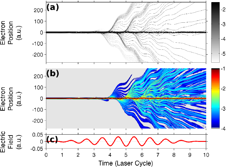
Figure 1: Comparison of the quantum trajectories (a) and the electron probability density (b) for the 1D model of H${}_{2}^{+}$ at $R=7$ for the interaction of H${}_{2}^{+}$ with an electric field (c) of a laser pulse (peak intensity $4\times 10^{13}$ W/cm², wavelength $1064$ nm, duration $T=10$ cycles, and CEP $\varphi=0$). In panel (a), the gray-scale color of each trajectory indicates $\log_{10}w_{j}$. In panel (b), the color code indicates $\log_{10}|\Psi|^{2}$, where $\Psi$ is obtained by solving the TDSE (7).

In Fig. 1 the Bohmian trajectories (Fig. 1(a)) are presented along with the electron probability density (Fig. 1 (b)) as a function of time. For the sake of comparison, the electric field of the laser pulse is shown in Fig. 1(c) as well. Subject to the intense electric field, the trajectories leave the core region (at $z\approx 0$) of the molecular ion in alternating directions ($z\rightarrow\pm\infty$) at every half cycle of the laser field. It is clearly seen that the number of ionizing trajectories increases as the field strength increases during the laser pulse. The trajectories liberated from the core region show wiggling motions forced by the alternating electric field of the laser. Due to this quiver motion, some of the trajectories, depending on the time instants of their release, are driven back to the core region and scattered off the protons. Please note that the results for the Bohmian trajectories visually agree very well with those for the electron probability density: regions of large probability density correspond to a large density of the Bohmian trajectories. Thus, the Bohmian trajectories provide a complete overall picture of the ionization process, including the quiver motion and the rescattering of the electron in the laser field. This agrees with the findings of earlier studies using Bohmian trajectories to describe the interaction of atoms with intense laser pulses Faisal and Schwengelbeck (1998); Lai et al. (2009a, b); Botheron and Pons (2010).

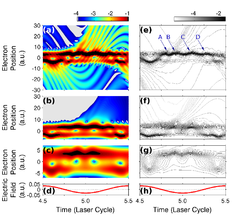
Figure 2: Close-up view on the time evolution of the electron probability density (a-c) and the quantum trajectories (e-g) over the single laser cycle at the pulse peak. The laser electric field is shown in panels (d) and (h) for comparison with the flow of the electron probability density and the quantum trajectories. In panels (a) and (d), no wavepacket absorber was set close to the core region. In panels (b) and (f), an absorber was set on one side of the core region at $-11<z<-7$. In panels (c) and (g), two absorbers were set on both sides of the core region at $7<|z|<11$.

In Fig. 2 we show a detailed view of the electron dynamics in and close to the core region (the protons are located at $z=\pm R/2=\pm 3.5$ a.u.) over the central field cycle ($T/2-2\pi/\omega<t<T/2+2\pi/\omega$) of the laser pulse using the electron probability density [Figs. 2(a)-2(c)] and the Bohmian trajectories [Figs. 2(e)-2(g)]. The laser electric field in the same time window is also shown in Figs. 2(d) and 2(h). In the simulations for Figs. 2(a) and 2(e), the wavefunction masks of $\cos^{1/4}$-shape were placed over $270<|z|<300$ only to avoid the reflection of the ionized wavepackets at the boundaries of the large simulation box, leaving the electron dynamics in the region of $z$ shown in these panels unaffected. Both of the electron probability density and the quantum trajectories show an ultrafast oscillatory motion around $5<|z|<10$ as indicated by, for example, the peaks A-D in Fig. 2(e). This oscillation involves the ionization and rescattering of the electron. To see this we suppressed the rescattering effect on the negative $z$-side by setting a wavefunction mask at $-11<z<-7$ for the simulations in Figs. 2(b) and 2(f) Burnett et al. (1998); Dörr (2000); Baier et al. (2006); Takemoto and Becker (2010). As a result, the peak A in Fig. 2(e) disappears in Fig. 2(f), indicating that this peak was created by the wavepacket driven back from $z<0$ and passing through the core region toward $z>0$. In Figs. 2(c) and 2(g), the wavefunction masks were set close to the core on both sides (at $7<|z|<11$) and all the rescattering wavepackets were absorbed after the initial ionization. The two peaks B and C in Fig. 2(e) are still present in Fig. 2(g) while peak D disappears, indicating that there are actually two bursts of ionization under the present conditions. These results confirm the previously reported phenomenon of multiple ionization bursts and attosecond electron localization Kawata et al. (1999); Takemoto and Becker (2010).

As in Fig. 1, the quantum trajectories reflect well the characteristics of the flow of the electron density in each pair of panels in Fig. 2. In addition, the quantum trajectories in Fig. 2(g) clearly elucidates that the electron probability moves back and forth between the two protons on the ultrafast time scale shorter than a half-cycle of the laser field. This is not as obvious in the plot of the electron probability density in Fig. 2(c). Thus, the quantum trajectories are shown to provide further insights in the flow of the probability density.

Please note that the electronic motion in Fig. 2(g) between the two potential wells created by the protons does not necessarily follow the laser-electron interaction potential $V_{\text{L}}$. For example, at $t=5$ cycles, the oscillating laser electric field $E(t)$ is peaked in the negative direction (cf. Fig. 2(h)), and hence the slope of $V_{\text{L}}$ pushing the electron toward $z\rightarrow+\infty$ becomes maximum. Nevertheless, we observe some bound trajectories propagated in the opposite direction from the proton located at $z=R/2=3.5$ to the other one at $z=-R/2=-3.5$ by climbing up the potential $V_{\text{L}}$. This counter-intuitive (and classically forbidden) motion of the electron was noticed first in the context of coherent control of electron localization in dissociating H${}_{2}^{+}$ molecule by the Wigner representation He et al. (2008). The present results confirm this motion and visualize it using Bohmian trajectories.

IV Analysis of the electron dynamics using Bohmian trajectories

We have seen so far that the Bohmian trajectories clearly visualize the transient electron localization and multiple ionization bursts within a half-cycle of the laser field oscillation. In this section we will now investigate the origin of the counter-intuitive motion of the Bohmian trajectories. To this end, we focus on the results for the intra-molecular electron transfer from one proton to the other, obtained by using wavepacket absorbers over $7<|z|<11$ in order to eliminate the effect of rescattering wavepackets (cf. Figs. 2(c) and 2(g)).

IV.1 Velocity field for the Bohmian trajectories

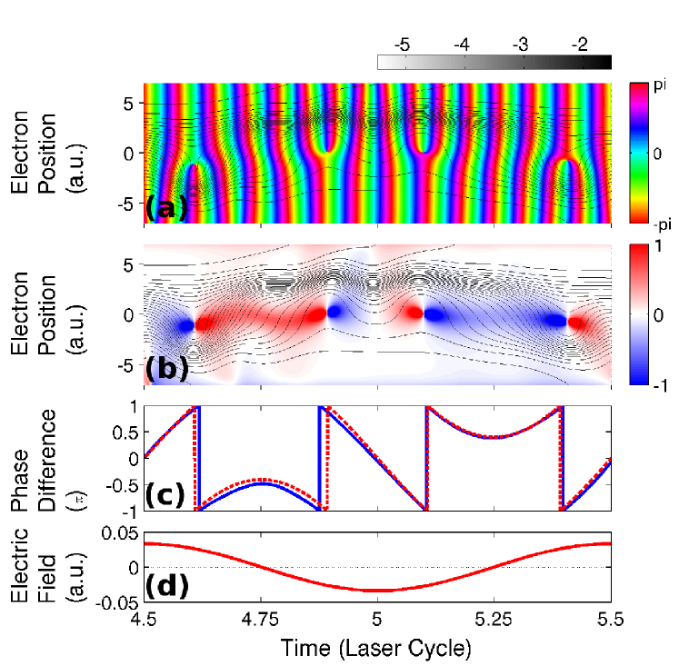
Figure 3: Analysis of the intra-molecular motion of the quantum trajectories in terms of the phase of the wavefunction $S(x,t)$ and the velocity field $v(x,t)$. (a) Phase $S(x,t)$ and the quantum trajectories $\{z_{j}(t)\}$. (b) Velocity field $v(x,t)$ and the quantum trajectories $\{z_{j}(t)\}$. (c) Phase difference between the two wells calculated from the 1D model ($\alpha_{\text{LR}}(t)$, blue solid line) and from the approximate solution of the two-state model ($\alpha_{\text{LR}}^{(\text{2lev})}(t)$, red dashed line). (d) Electric field of the laser pulse (wavelength $1064$ nm, peak intensity $4\times 10^{13}$ W/cm², duration $T=10$ cycles, and CEP $\phi=0$).

As pointed out before, we observe that some of the trajectories turn their direction toward $z<0$ near the peak of the electric field at $t=5$ cycles while the classical force due to the laser electric field pushes the electron in the positive $z$ direction. We now investigate this counter-intuitive motion in terms of the velocity field, $v(x,t)=\partial S(x,t)/\partial x$, for the Bohmian trajectories. Fig. 3(a) shows the phase $S(x,t)$ of the wavefunction and Fig. 3(b) the velocity field $v(x,t)$ both calculated using the same parameters of the field as before. In both Figures we superposed the Bohmian trajectories for further visualization.

From Fig. 3(a), we can notice that at a given time instant the phase of the wavefunction is almost constant within each of the potential wells. However, the phase propagates at different speeds in the two wells. This causes a phase gradient around $z=0$ and, consequently, a large absolute value of the velocity field in the region between the protons. Over the central half ($4.75<t<5.25$ laser cycles) of the field cycle shown in Fig. 3, the velocity field changes its sign at $t=4.89$, $5.0$, and $5.10$ laser cycles and, hence, forces the Bohmian trajectories to turn their direction at these instants. The change of sign of the velocity field corresponds to those instants at which the accumulated phase difference between the two wells equals a multiple of $\pi$. This interpretation is confirmed by the results for the relative phase of the wavefunction, defined as

$$\alpha_{\text{LR}}(t)=\arg\left[\Psi\left(z=-\frac{R}{2},t\right)\right]-\arg\left[\Psi\left(z=\frac{R}{2},t\right)\right],$$ (14)

and shown as solid line in Fig. 3(c). One can clearly see that every jump in the relative phase $\alpha_{\text{LR}}$ from $-\pi$ to $\pi$ corresponds to an abrupt sign change of $v(x,t)$. We may note that this divergence of the $v(x,t)$ is accompanied by a node in the wavefunction at the same position [cf. Fig. 2(c)], and that therefore the flux $v(x,t)|\Psi(x,t)|^{2}$ stays finite. The phase jump between $-\pi$ and $\pi$ can be interpreted as following: If the local phase at one well gets more and more retarded (or advanced) from that at the other well and if the absolute difference passes $\pi$, then the former should be now regarded as more advanced (retarded) than the latter.

IV.2 Phase difference in two-state model

Next, we show that the phase difference $\alpha_{\text{LR}}$ can be approximated by a simple expression based on a two-state model. To this end, we analyze the relative phase between the two potential wells in terms of the following localized states Kayanuma (1993, 1994); Creffield (2003),

$$|\text{L}\rangle= \frac{1}{\sqrt{2}}\left[|\text{g}\rangle+|\text{u}\rangle\right],$$ (15)

$$|\text{R}\rangle= \frac{1}{\sqrt{2}}\left[|\text{g}\rangle-|\text{u}\rangle\right],$$ (16)

where $|\text{g}\rangle$ and $|\text{u}\rangle$ are the ground and first-excited electronic states, respectively, of the 1D fixed-nuclei model. Without loss of generality, we set the phases of $|\text{g}\rangle$ and $|\text{u}\rangle$ such that $|\text{L}\rangle$ and $|\text{R}\rangle$ are localized at $z=-R/2$ and $z=R/2$, respectively. By approximating the state of the system in the basis of these two localized states as $|\Psi(t)\rangle=c_{\text{L}}(t)|\text{L}\rangle+c_{\text{R}}(t)|\text{R}\rangle$, the time-evolution of $c_{\text{L}}(t)$ and $c_{\text{R}}(t)$ is given by

$$i\frac{d}{dt}\begin{pmatrix}c_{\text{L}}\\ c_{\text{R}}\end{pmatrix}=\left[H^{(\text{2lev})}_{0}+V^{(\text{2lev})}_{\text{L}}\right]\begin{pmatrix}c_{\text{L}}\\ c_{\text{R}}\end{pmatrix},$$ (17)

with the field-free Hamiltonian

$$H^{(\text{2lev})}_{0}=-\frac{\Delta_{0}}{2}\begin{pmatrix}0&1\\ 1&0\end{pmatrix},$$ (18)

and the interaction potential

$$V^{(\text{2lev})}_{\text{L}}=-d_{\text{gu}}E(t)\begin{pmatrix}1&0\\ 0&-1\end{pmatrix},$$ (19)

where $\Delta_{0}$ is the absolute value of the difference between the field-free energies of $|\text{u}\rangle$ and $|\text{g}\rangle$, and $d_{\text{gu}}=-\langle\text{g}|z|\text{u}\rangle\geq 0$ is the transition dipole moment between $|\text{g}\rangle$ and $|\text{u}\rangle$.

If the laser-molecule coupling $|d_{gu}E(t)|$ is sufficiently strong and/or the laser frequency $\omega$ is sufficiently larger than the tunnel splitting $\Delta_{0}$, we may approximate the solution to the two-state TDSE (17) by taking $V^{(\text{2lev})}_{\text{L}}$ as the zeroth order reference Hamiltonian and omitting the $H_{0}$ term Grossmann et al. (1991); Großmann and Hänggi (1992); Yu. Ivanov and Corkum (1993); Yu. Ivanov et al. (1993); Burdov (1997); Creffield (2003); Santana et al. (2001). Such a zeroth order solution can be easily obtained as Creffield (2003)

$$c^{(0)}_{\text{L}}(t)= \exp\left\{-id_{\text{gu}}[A(t)-A(t_{0})]\right\}c^{(0)}_{\text{L}}(t_{0}),$$ (20)

$$c^{(0)}_{\text{R}}(t)= \exp\left\{id_{\text{gu}}[A(t)-A(t_{0})]\right\}c^{(0)}_{\text{R}}(t_{0}),$$ (21)

where the relation of the electric field and vector potential, Eq. (4), was used. Then, the phase difference between the two wells can be approximated by

$$\alpha^{(\text{2lev})}_{\text{LR}}(t)=\arg\left[c^{(0)}_{\text{L}}\right]-\arg\left[c^{(0)}_{\text{R}}\right].$$ (22)

By substituting Eqs. (20) and (21) into Eq. (22), and noting that $A(t_{0})=0$ at the beginning of the laser pulse at $t=t_{0}=0$, we obtain

$$\alpha^{(\text{2lev})}_{\text{LR}}(t)=-2d_{\text{gu}}A(t)+\alpha^{(\text{2lev})}_{\text{LR}}(t_{0}).$$ (23)

The phase difference calculated by this expression is plotted in Fig. 3(c) as the red dashed line. We can see that the two-state model closely reproduces the exact value (blue solid line) calculated numerically by Eq. (14).

The condition, $\alpha_{\text{LR}}^{(\text{2lev})}(t_{\text{turn}})=n\pi$, $n\in\mathbb{Z}$, for the time instant $t_{\text{turn}}$ at which the velocity field between the two protons changes its sign is then given by

$$A(t_{\text{turn}})=\frac{-n\pi+\alpha^{(\text{2lev})}_{\text{LR}}(t_{0})}{2d_{\text{gu}}}.$$ (24)

This expression has a similar form as the condition for the time instant $t_{\text{loc}}$ of maximum electron localization,

$$A(t_{\text{loc}})=\frac{m\pi+\chi}{2d_{\text{gu}}},$$ (25)

with $m\in\mathbb{Z}$ derived previously Takemoto and Becker (2010) based on the series expansion of the Floquet states for the two-state model Santana et al. (2001). In fact, these two expressions are identical at the limit of long laser pulse duration where the mixing angle $\chi$ of the two Floquet states reduces to the initial phase difference $\alpha^{(\text{2lev})}_{\text{LR}}(t_{0})$.

IV.3 Origin of the counter-intuitive electron motion

The result of the two-state analysis in the previous subsection, in which we consider $V^{(\text{2lev})}_{\text{L}}$ as the zeroth order Hamiltonian while neglecting the tunnel hopping term $H_{0}$, provides us with an intuitive picture. Please note that the transition dipole moment has the asymptotic form $d_{\text{gu}}\sim R/2$ at large $R$ Mulliken (1939), and the difference of the diagonal elements of $V^{(\text{2lev})}$ is, hence, approximately equal to $RE(t)$, which is the difference of the electric potential induced by the laser field between the two wells. Using this asymptotic form of $d_{\text{gu}}$, the phase difference in Eq. (23) can be rewritten as

$$\alpha^{(\text{2lev})}_{\text{LR}}(t)\sim\int_{t_{0}}^{t}dt^{\prime}RE(t^{\prime})+\alpha^{(\text{2lev})}_{\text{LR}}(t_{0}).$$ (26)

This expression elucidates that the origin of the phase difference between the two potential wells, and hence the velocity field, is the difference of the electric potential energies between the two wells induced by the laser light.

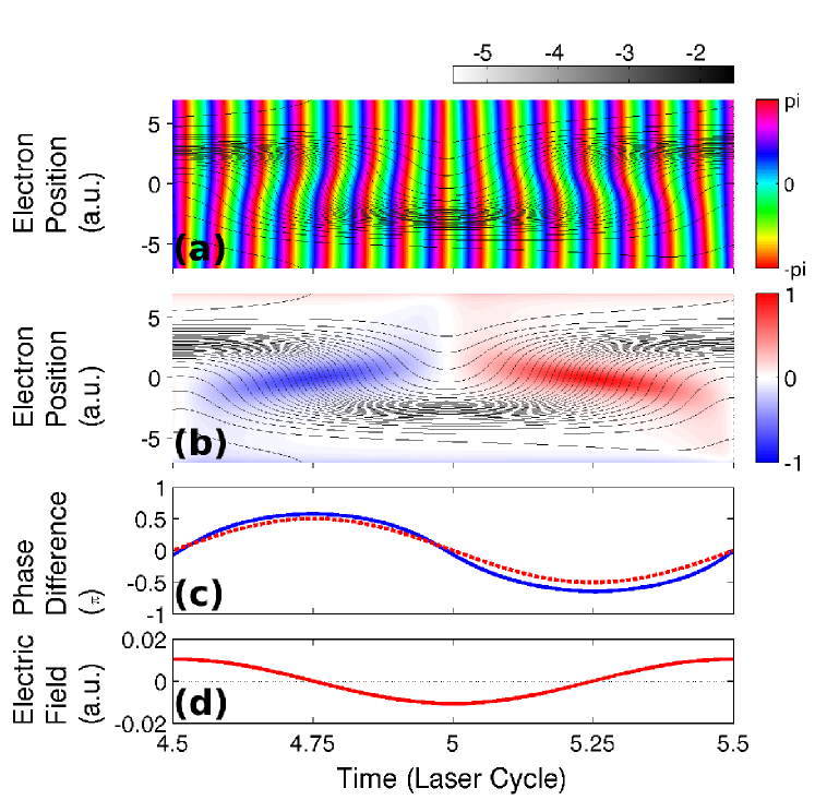
Figure 4: Time evolutions of (a) the phase of the wavefunction and (b) the velocity field are plotted along with the quantum trajectories. The system was initially prepared in the ground state $|\text{g}\rangle$. Panel (c) shows the phase difference between the two local potential wells calculated from the TDSE solution (blue solid line) and from the two-state model (red dashed line). Panel (d) shows the electric field of the laser pulse (wavelength $1064$ nm, peak intensity $4\times 10^{12}$ W/cm², duration $T=10$ cycles, and CEP $\phi=0$).

This interpretation of the electronic dynamics based on the zeroth order two-state analysis predicts that the motion of the electron should be still counter-intuitive even at a relatively low intensity at which only one localization per half-cycle is predicted by Eq. (24) or (25). This is demonstrated in Fig. 4 in which the 1D model was initially prepared in the ground state, and a laser pulse of peak intensity $4\times 10^{12}$ W/cm² was applied. The other parameters were the same as above. The initial phase difference $\alpha^{(\text{2lev})}_{\text{LR}}(t_{0})$ is zero due to the choice of the initial state as $|\text{g}\rangle$, and the velocity field around $z=0$ evoles in time as $-A(t)$ according to the two-state analysis (Fig. 4(c)). Due to the phase-lag between $A(t)$ and $E(t)$, the quantum trajectories are navigated from $z=R/2$ to $z=-R/2$ during the $4.5<t<5$, for example, while the electric force $-E(t)$ points in the opposite direction during $4.75<t<5$. As a consequence, the trajectories are always accumulated at the upper potential well, in contradiction to our classical intuition.

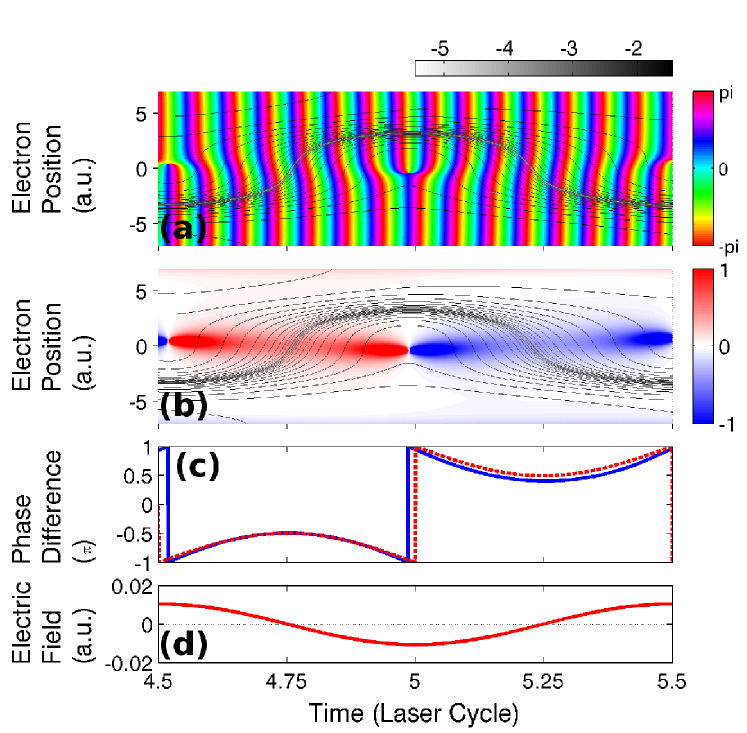
Figure 5: Same as Fig. 4 except that here the system was initially prepared in the first excited state $|\text{u}\rangle$.

If, instead, the system is initially prepared in the first excited state $|\text{u}\rangle$, the initial phase difference $\alpha^{(\text{2lev})}_{\text{LR}}(t_{0})=-\pi$. Due to this offset, the quantum trajectories (and the electron probability density) are navigated toward the lower potential well in this case. In fact, we can see that this is the case for the results presented in Fig. 5 where we applied the same laser pulse as used for the results shown in Fig. 4 but prepared the system in the 1D model of H${}_{2}^{+}$ in the first excited state.

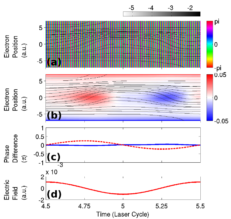
Figure 6: Same as Fig. 4 except that here a laser pulse with long wavelength ($5000$ nm) and low intensity ($4\times 10^{10}$ W/cm²) (duration $T=10$ cyc, CEP $\phi=0$) was applied.

We may finally ask if there is a parameter regime in which our intuitive (classical) picture that the electron should move in the direction of the electric force is always recovered. As we mentioned above, our two-state analysis is based on the assumption that $V^{(\text{2lev})}_{\text{L}}$ is the dominant term, i.e. that the laser-molecule coupling is strong and/or the photon energy is sufficiently larger than the tunnel splitting. Please note that the photon energy at the wavelength of $1064$ nm is $\omega=0.043$, whereas the tunnel splitting is $\Delta_{0}=0.028$ for the 1D model at $R=7$. If we decrease the photon energy as well as the laser intensity, the two-state analysis is no longer applicable. In fact, the results in Fig. 6 show that at a wavelength of $5000$ nm and an intensity of $4\times 10^{10}$ W/cm² our two-state analysis breaks down, since the phase difference $\alpha^{(\text{2lev})}_{\text{LR}}(t)$ (red dashed line) predicted by the two-state analysis deviates qualitatively from the value of $\alpha_{\text{LR}}(t)$ (blue solid line) calculated from the TDSE solution (Fig. 6(c)). We can see that in this parameter regime, in which the conventional weak field perturbation theory may be applied, the motion of the quantum trajectories (and the electron probability density) follows the electric force of the laser field, and the intuitive (classical) picture is indeed recovered.

V Conclusions

We have presented an analysis of the attosecond electron dynamics in hydrogen molecular ion driven by an intense laser pulse in terms of Bohmian trajectory calculations using a 1D model. Results of these calculations are found to be in good overall agreement with those of numerical simulations of the TDSE. Recently predicted phenomena such attosecond transient electron localization and multiple bursts of ionization within a half cycle of the laser pulse are clearly represented by the Bohmian trajectories. Further analysis let us identify the origin of the sometimes counter-intuitive motion of the Bohmian trajectories as due to the time evolving phase difference of the wavefunction between the two potential wells induced by the electric potential of the laser field. We were able to predict the time instants at which the trajectories change their directions within a simple two-state model. Following our analysis we showed that exposed to an intense laser field the electron dynamics in the hydrogen molecular ion often does not follow the (classical) force of the laser electric field. Our classical expectations are however recovered in the perturbative weak-field limit in which the photon energy and intensity of the laser field are both sufficiently small.

References

- Bohm (1952a) D. Bohm, Phys. Rev. 85, 166 (1952a).
- Bohm (1952b) D. Bohm, Phys. Rev. 85, 180 (1952b).
- Holland (1993) P. R. Holland, The Quantum Theory of Motion: An Account of the de Broglie-Bohm Causal Interpretation of Quantum Mechanics (Cambridge University Press, 1993).
- Wyatt (2005) R. E. Wyatt, Quantum Dynamics with Trajectories: Introduction to Quantum Hydrodynamics (Springer, 2005).
- Kawata et al. (1999) I. Kawata, H. Kono, and Y. Fujimura, J. Chem. Phys. 110, 11152 (1999).
- He et al. (2008) F. He, A. Becker, and U. Thumm, Phys. Rev. Lett. 101, 213002 (2008).
- Takemoto and Becker (2010) N. Takemoto and A. Becker, Phys. Rev. Lett. 105, 203004 (2010).
- Zuo and Bandrauk (1995) T. Zuo and A. D. Bandrauk, Phys. Rev. A 52, R2511 (1995).
- Mulliken (1939) R. S. Mulliken, J. Chem. Phys. 7, 20 (1939).
- Hu et al. (2009) S. X. Hu, L. A. Collins, and B. I. Schneider, Phys. Rev. A 80, 023426 (2009).
- Chelkowski et al. (1995) S. Chelkowski, O. A. T. Zuo, and A. D. Bandrauk, Phys. Rev. A 52, 2977 (1995).
- Roudnev et al. (2004) V. Roudnev, B. D. Esry, and I. Ben-Itzhak, Phys. Rev. Lett. 93, 163601 (2004).
- He et al. (2007) F. He, C. Ruiz, and A. Becker, Phys. Rev. Lett. 99, 083002 (2007).
- (14) N. Takemoto and A. Becker, to be published.
- Javanainen et al. (1988) J. Javanainen, J. H. Eberly, and Q. Su, Phys. Rev. A 38, 3430 (1988).
- Kulander et al. (1996) K. C. Kulander, F. H. Mies, and K. J. Schafer, Phys. Rev. A 53, 2562 (1996).
- Marston and Balint-Kurti (1989) C. C. Marston and G. G. Balint-Kurti, J. Chem. Phys. 91, 3571 (1989).
- Bandrauk and Shen (1993) A. D. Bandrauk and H. Shen, J. Chem. Phys. 99, 1185 (1993).
- Takahashi and Ikeda (1993) K. Takahashi and K. Ikeda, J. Chem. Phys. 99, 8680 (1993).
- Press et al. (1992) W. H. Press, S. A. Teukolsky, W. T. Vetterling, and B. P. Flannery, Numerical Recipes in Fortran 77: The Art of Scientific Computing, Vol. 1 of Fortran Numerical Recipes (Cambridge University Press, New York, 1992), 2nd ed.
- Garashchuk and Rassolov (2002) S. Garashchuk and V. A. Rassolov, Chem. Phys. Lett. 364, 562 (2002).
- Garashchuk and Rassolov (2003) S. Garashchuk and V. A. Rassolov, J. Chem. Phys. 118, 2482 (2003).
- Lopreore and Wyatt (1999) C. L. Lopreore and R. E. Wyatt, Phys. Rev. Lett. 82, 5190 (1999).
- Mayor et al. (1999) F. S. Mayor, A. Askar, and H. A. Rabitz, J. Chem. Phys. 111, 2423 (1999).
- Poirier (2010) B. Poirier, Chem. Phys. 370, 4 (2010).
- Botheron and Pons (2010) P. Botheron and B. Pons, Phys. Rev. A 82, 021404(R) (2010).
- Sharp (1970) T. Sharp, At. Data Nuc. Data Tables 2, 119 (1970).
- Faisal and Schwengelbeck (1998) F. Faisal and U. Schwengelbeck, Pramana 51, 585 (1998).
- Lai et al. (2009a) X. Y. Lai, Q. Y. Cai, and M. S. Zhan, Eur. Phys. J. D 53, 393 (2009a).
- Lai et al. (2009b) X. Y. Lai, Q.-Y. Cai, and M. S. Zhan, New J. Phys. 11, 113035 (2009b).
- Burnett et al. (1998) K. Burnett, J. B. Watson, A. Sanpera, and P. L. Knight, Phil. Trans. Roy. Soc. London A 356, 317 (1998).
- Dörr (2000) M. Dörr, Opt. Express 6, 111 (2000).
- Baier et al. (2006) S. Baier, C. Ruiz, L. Plaja, and A. Becker, Phys. Rev. A 74, 033405 (2006).
- Kayanuma (1993) Y. Kayanuma, Phys. Rev. B 47, 9940 (1993).
- Kayanuma (1994) Y. Kayanuma, Phys. Rev. A 50, 843 (1994).
- Creffield (2003) C. Creffield, Phys. Rev. B 67, 165301 (2003).
- Grossmann et al. (1991) F. Grossmann, T. Dittrich, P. Jung, and P. Hänggi, Phys. Rev. Lett. 67, 516 (1991).
- Großmann and Hänggi (1992) F. Großmann and P. Hänggi, Europhys. Lett. 18, 571 (1992).
- Yu. Ivanov and Corkum (1993) M. Yu. Ivanov and P. B. Corkum, Phys. Rev. A 48, 580 (1993).
- Yu. Ivanov et al. (1993) M. Yu. Ivanov, P. B. Corkum, and P. Dietrich, Laser Phys. 3, 375 (1993).
- Burdov (1997) V. A. Burdov, JETP 85, 657 (1997).
- Santana et al. (2001) A. Santana, J. M. Gomez Llorente, and V. Delgado, J. Phys. B 34, 2371 (2001).