The Generalized Quantization Schemes for Games and its Application to Quantum Information

Abstract

Theory of quantum games is relatively new to the literature and its applications to various areas of research are being explored. It is a novel interpretation of strategies and decisions in quantum domain. In the earlier work on quantum games considerable attention was given to the resolution of dilemmas present in corresponding classical games. Two separate quantum schemes were presented by Eisert et al. [27] and Marinatto and Weber [28] to resolve dilemmas in Prisoners’ Dilemma and Battle of Sexes games respectively. However for the latter scheme it was argued [39] that dilemma was not resolved. We have modified the quantization scheme of Marinatto and Weber to resolve the dilemma. We have developed a generalized quantization scheme for two person non-zero sum games which reduces to the existing schemes under certain conditions. Applications of this generalized quantization scheme to quantum information theory are studied. Measurement being ubiquitous in quantum mechanics can not be ignored in quantum games. With the help of generalized quantization scheme we have analyzed the effects of measurement on quantum games. Qubits are the important elements for playing quantum games and are generally prone to decoherence due to their interactions with environment. An analysis of quantum games in presence of quantum correlated noise is performed in the context of generalized quantization scheme. Quantum key distribution is one of the key issues of quantum information theory for the purpose of secure communication. Using mathematical framework of generalized quantization scheme we have proposed a protocol for quantum key distribution. This protocol is capable of transmitting four symbols for key distribution using a two dimensional quantum system. Quantum state tomography has a substantial place in quantum information theory. Much like its classical counterpart, its aim is to reconstruct a three dimensional image through a series of different measurements. Making use of the mathematical framework of generalized quantization scheme we have presented a technique for quantum state tomography.

All glory be to Allah who helped me to manage the unmanageable.

I am extremely grateful to my supervisor, Dr. Abdul Hameed Toor for his invaluable assistance, expert guidance, amiable mood and the provision of friendly and affable environment during the entire research work on and off the campus. A huge note of thanks must go to my teachers Dr. Azhar Abbas Rizvi, Dr. Farhan Saif, Dr. Qaiser Naqvi and all other faculty members of the Department of Electronics, Quaid-i-Azam University Islamabad for their help and guidance during my course work. I am extremely thankful to Dr. Azhar Iqbal for introducing me to the fascinating field of quantum game theory and for motivating discussions on the subject. I am very grateful to Prof. János A. Bergou for his helpful suggestions and invaluable discussions on quantum information theory during his visit to Pakistan. An honourable note of thanks must go to Prof. Dr. Moiz Hussain who taught me to be determined, concentrated and feisty in complicated, impenetrable and challenging situations of life.

My respectful thanks are also due to my senior colleagues Dr. Altaf Hussain, Mr. Ejaz Ahmad Mukhtar, Mr. Fahim Ahmad and Mr. Shahid Noman-ul-Haq for providing me the opportunity and facilities for studies. To my friends and colleagues, Mr. Khalil Ahmad, Mr. Muhammad Azam Ghori, Mr. Muhammad Salim, Mr. Muhammad Qadir Asad, Mr. Athar Rasool, Mr. Muhammad Israr Khan, Mr. Muhammad Iqbal and Z. Z. Bhatty- thank you for your constant encouragement, empowering remarks, regular inspiration and stimulating discussions in these challenging hours of my life. I am very thankful to my best friends and caring fellows Mr. Mehboob Hussain, Mr. Mustansar Nadeem and Miss. Nigum Arshed whose company imparted me indelible memories and converted my stay at university into a memorable time of my life.

How can I forget my mother at this occasion who always prayed for my success and never complained about my long absence during the research period. Thank you, mother! thanks a lot. I am very grateful to my brothers Mr. Ayaz Khan, Mr. Haroon Khan, Mr. Sheraz Khan, Mr. Aamer Shehzad and sisters for their support and care during these busy hours. At last and not at least I am thankful to my wife, Saima Rasti and children, Minahil Yaqub, Laiba Yaqub and Muhammad Obaidullah Yaqub who energized me with their innocent remarks and kept me reminding that there is also a world outside the academia.

This thesis is based on the following publications:

• Ahmad Nawaz and A. H. Toor, Dilemma and quantum battle of sexes, J. Phys. A: Math. Gen. 37, 4437 (2004).

• Ahmad Nawaz and A. H. Toor, Generalized quantization scheme for two person non-zero sum game, J. Phys. A: Math. Gen. 37, 11457 (2004).

• Ahmad Nawaz and A. H. Toor, Role of measurement in quantum games, J. Phys. A: Math. Gen. 39, 2791 (2006).

• Ahmad Nawaz and A. H. Toor, Quantum games with correlated noise, J. Phys. A: Math. Gen. 39, 9321 (2006).

• Ahmad Nawaz, A. H. Toor and J. Bergou, Efficient quantum key distribution: submitted.

• Ahmad Nawaz and A. H. Toor, Quantum games and quantum state tomography: in preparation.

Chapter 1 Introduction

Game theory deals with the situations where two (or more) players or the decision makers compete to maximize their respective gains. The player’s gain known as payoff can be in the form of money or some sort of spiritual happiness which one feels on one’s success. The players are rational in nature therefore, while taking any action to achieve their objectives they keep an eye on the expectations and objectives of the other players and they also know well the strategies to achieve these objectives [1]. Furthermore these interactions are strategic in nature as the payoff of one player depends on his own and as well as on the strategies adopted by other player/players [2]. The strategy of players is a complete plan of actions depending on the sensitivity and nature of a particular situation (game). The rational reasoning of the players for selection of those strategies that maximizes their payoffs decides the outcome of a game. A set of strategies from which unilateral deviation of a player reduces his/her payoff is called Nash equilibrium (NE) of the game which is a key concept in the solution of a game [3].

Game theory was developed by von Neumann and Morgenstern [2] and John Nash [3] as a tool to understand economic behaviors. Since then it has been widely used in various fields including warfare, anthropology, social psychology, economics, politics, business, international relations, philosophy and biology. It is also used by computer scientists in artificial intelligence [4, 5] and cybernetics [6, 7]. There is an increasing interest in applying the game theoretic concepts to physics [8]. Some algorithms and protocols of quantum information theory has also been formulated in the language of game theory [9, 10, 11, 12, 13, 14].

The problems of classical game theory can be implemented into an experimental (physical) set-up by using classical bits. A classical bit can be represented by any two level system such as a coin i.e. it can be encoded on any system that can take one of the two distinct possible values. For example a bit on a compact disk means whether a laser beam is reflected or not reflected from its surface. A bit is represented by the Boolean states $0$ and $1$. To play two players classical games experimentally we need an arbiter having two similar coins in same state. He hands over a coin to each of the player. The strategies of the players are to flip or not to flip the coin. The players return their coins to arbiter after playing the respective strategies. Checking the state of coins the arbiter announces the payoffs for players using the payoff matrix known to both the players.

Quantum games, on the other hand, are played using quantum bits (qubits) and the qubits are much different than their classical counterpart. A qubit is a microscopic system such as an electron or nuclear spin or a polarized photon. In this case the Boolean states $0$ and $1\$are represented by a pair of reliably distinguished states of the qubit [15]. Spin up and spin down of an electron or the horizontal and vertical polarizations of photon are very remarkable examples in this regard. Qubits can exist in form of superposition in two dimensional Hilbert space spanned by the unit vectors. Furthermore qubits can also exist in a state totally different than classical states called entangled state. Computers that work on the basis of these quantum resources are known as quantum computers [16, 17, 18, 19, 20, 21]. Extensive study of quantum computation motivated the study of quantum information theory. This relatively new research field taught to think physically about computation and provided with the exciting capabilities for the information storage, processing and communication [22]. Processing of information in quantum domain started an interesting debate among scientists for faster than light communication, a task that is impossible according the Einstein’s theory of relativity [23]. It was directly linked to a question whether it was possible to clone an unknown quantum state. However, no cloning theorem [24] proved that the task that was easy to accomplish with classical information is impossible for quantum information. Quantum information theory gave a new brand of cryptography where security does not depend upon the computational complexity but depends upon fundamental physics and introduced quantum computers that can provide the mathematical solutions to certain problems very fast. It is stated that information theory based on quantum principles extends and completes the classical information theory just as the complex numbers extend and complete the real numbers [15, 25]. These fascinating ideas led to translate the problems of game theory into physical set-up that uses qubits instead of classical bits [26, 27, 28].

Quantum game theory started with an interesting story of success of a hypothetical quantum player over a classical player in quantum penny flip game [26]. David Meyer described this game by the story of a spaceship which faces a catastrophe during its journey. Suddenly a quantum being, Q, appears to help save the spaceship if Picard, the captain of the spaceship, beats him in a penny flipping game. According to the game, Picard is to place the penny with head up in a box. Q has an option to either flip the penny or leave it unchanged without looking at it. Then Picard has the same options without having a look at the penny. Finally Q takes the turn with the same options without looking at the penny. If in the end penny is head up then Q wins otherwise Picard wins. Captain Picard being expert of game theory knows that this game has no deterministic solution and deterministic Nash equilibrium [2, 3]. In other words, there exist no such pair of pure strategies from which unilateral withdrawal of any player can enhance his/her payoff. Therefore, he agrees to play with Q. But to Picard’s surprise, Q always wins. Since the quantum being Q is capable of playing quantum strategies which is the superposition of head and tail in the two dimensional Hilbert space, thus he is always the winner.

In non-zero sum classical games Nash equilibrium (NE) is central to analysis, however, this concept has some shortcomings as well. First, it is not necessarily true that each game has a unique Nash equilibrium. There are examples of the games with multiple Nash equilibria where the players cannot choose the Nash equilibrium e.g. Battle of Sexes and Chicken games. Second, in some cases Nash equilibrium could result outcomes being very far from the benefit of players. Prisoners’ Dilemma is an interesting example depicting such a situation where the players trying to maximize their respective payoffs fall in a dilemma and end up with worst outcomes. Quantum game theory helps resolve such dilemmas [27, 28] and shows that quantum strategies can be advantageous over classical strategies [26, 27, 29]. To deal with such situations one of the foremost and elegant quantization schemes is introduced by Eisert et al. [27] taking Prisoners’ Dilemma as an example. In this quantization scheme the strategy space of the players is a two parameter set of $2\times 2$ unitary matrices. Starting with maximally entangled initial quantum state the authors showed that for a suitable quantum strategy the dilemma disappears. They also pointed out a quantum strategy which always wins over all the classical strategies. Marinatto and Weber [28] introduced another interesting and simple scheme for the analysis of non-zero sum classical games in quantum domain. They gave Hilbert structure to the strategic spaces of the players. They used maximally entangled initial state and allowed the players to play their tactics by applying probabilistic choice of unitary operators. They applied their scheme to an interesting game of Battle of Sexes and found out the strategy for which both the players can achieve equal payoffs. Both Eisert’s and Marinatto and Weber’s schemes give interesting results for various quantum analogue of classical games [29, 30, 31, 32, 33, 34].

Meyer [26, 35], in his pioneering work pointed out a connection between quantum games and quantum information processing. Lee and Johnson [36] presented a game theoretic model for quantum state estimation and quantum cloning. They also developed a connection between quantum games and quantum algorithms [37]. In this thesis we introduced a generalized quantization scheme for two person non zero sum games and by using the mathematical framework of this generalized quantization scheme (chap. 6) we have proposed an efficient protocol for quantum key distribution. This protocol can be used to transmit four symbols for key distribution between sender and receiver using a two dimensional system, whereas in other quantum key distribution schemes higher dimensional systems are used for this purpose [38]. Using the framework of generalized quantization scheme a protocol for quantum state tomography is also presented. It can safely be stated that this work is a step forward for strengthening the established link between quantum games and quantum information theory.

Thesis Layout and Statement of Original Contribution

Chapter 2 is a brief introduction to classical game theory while chapter 3 contains some basic concepts of quantum mechanics required to understand quantum games. Chapter 4 and chapter 5 give reviews of quantum game theory and quantum information theory respectively.

In section (4.4) we show that the worst case payoffs scenario in quantum Battle of Sexes, as pointed out by Benjamin [39], is not due to the quantization scheme itself but it is due to the restriction on the initial state parameters of the game. If the game is allowed to start from a more general initial entangled state then a condition on the initial state parameters can be set such that the payoffs for the mismatched or the worst case situation are different for different players which results in a unique solution of the game.

Chapter 6 deals with the generalized quantization scheme for two person non-zero sum games which gives a relationship between Eisert et al. [27] and Marinatto and Weber [28] quantization schemes. Separate set of parameters are identified for which this scheme reduces to that of Marinatto and Weber and Eisert et al. schemes. Furthermore there have been identified some other interesting situations which are not apparent within the exiting quantizations schemes. In section (LABEL:measurement) the effects of measurement on quantum games are analyzed under the generalized quantization scheme. It is observed that as in the case of quantum channel capacities [40] , one can have four types of payoffs in quantum games for different combinations of input states and measurement basis. Furthermore a relation among these payoffs is also established.

In chapter 7 we analyze quantum games in presence of quantum correlated dephasing channel in the context of our generalized quantization scheme for non-zero sum games. It is shown that in the limit of maximum correlation the effect of decoherence vanishes and the quantum game behaves as a noiseless game.

In chapter 8 and 9, using the mathematical framework of generalized quantization scheme, we present protocols for quantum key distribution and quantum state tomography respectively.

Chapter 2 Game Theory

Game theory provides us with mathematical tools to help understand the phenomena that we observe when two or more players with conflicting interests interact. The physical situations arising in daily life are represented by abstract models and the contestants are supposed to be rational in nature who reason strategically [1, 41, 42]. Players play their strategies while keeping an eye on the objectives and expectations of other players and hence the resulted payoffs are functions of the strategies adopted by all the players involved in the contest.

In the following some basic definitions and terminology required to help understand the mathematical models of game theory are given following with some interesting examples from classical game theory. For these definitions and examples we consulted the Refs. [1, 41, 42].

2.1 Basic Definitions

Game:- A game consists of a set of players, a set of rules that dictates what actions the players can perform and a payoff function that tells about the reward of a player against given set of strategies. Mathematically it is a triple $\left(N,\Omega,\$\right)$ where $N$ is the number of players, $\Omega=_{\times k}\Omega$ with $1\leq k\leq N$ such that each $\ \Omega_{k}$ is the set of strategies for the $kth$ player and $\$:\Omega\longrightarrow R^{N}$ where $\$$ is the payoff of the $kth$ player.

Player:- In all game theoretic models the basic entity of a game is a player. It is an agent taking part in a game. Player can be an individual or a set of individuals.

Payoff:-These are the real numbers associated with each possible outcome of a game.

Move:- These are the actions or choices available to a player in a game.

Strategy:- It is the complete plan of actions of players for all possible circumstances during the course of the play.

Pure strategy:- Pure strategy is a nonrandom course of action for players. These are the moves that are specified without any uncertainty. Unless otherwise stated a strategy refers to a pure strategy.

Mixed strategy:- This is a rule that tells the player to use each or some of their pure strategies with specific probabilities.

Dominant strategy:- A pure strategy is referred to as dominant strategy if it results higher payoff than any alternate strategy for all possible choices of the opposing players. Mathematically a strategy $i$ is dominant strategy of player $i$ if

$$\$_{i}(s_{1},\text{......}s_{i-1},s_{i},\text{......}s_{n})\geq\$_{i}(s_{1},\text{.....}s_{i-1},\acute{s}_{i},.\text{......}s_{n}).$$

Rationality:- Reasoning strategically while keeping an eye on the objects and expectations of other players.

Zero sum game:- A game is zero-sum if the sum of the players’ payoffs is always zero. A two players zero sum game is also called a duel.

Non zero sum game:- A game in which the sum of the players’ payoffs is not zero.

Information:- What each player knows at each point of a game. Information may be perfect or imperfect, symmetric or asymmetric, complete or incomplete and certain or uncertain.

Symmetric game:- A game $G=(I,S,\$)$ is a symmetric two player game if $I=\{1,2\}$, $S_{1}=S_{2}$ and $\$_{2}\left(s_{1},s_{2}\right)=\$_{2}\left(s_{2},s_{1}\right)$ for all $\left(s_{1},s_{2}\right)\in S.$ In symmetric games all the players face exactly the same choices and exactly the same outcomes associated with their choices. Otherwise the game is asymmetric.

Nash equilibrium (NE):- It is set of strategies from which unilateral deviation of a player reduces his/her payoff.

Maximin:- The largest minimum payoff in a zero sum game.

Minimax:- The smallest maximum payoff in a zero sum game.

Pareto optimal (PO):- A solution set is Pareto Optimal means that there are no other solutions in which all the players simultaneously do better.

Evolutionary stable strategy (ESS):- The concept of ESS is refinement to Nash equilibrium. An ESS is a strategy if adopted by a population then no mutants can invade it by playing any other strategy.

Sequential games:- These are the game where the players act on strict turns.

Simultaneous games:- These are the games where the players act at the same time.

2.2 Representation of Games

There are different ways to represent a game, however, the following two ways are most commonly used [43].

2.2.1 Normal Form

In the normal form the game is represented by a payoff matrix which shows the players, strategies and payoffs. This representation is also called strategic form representation. The normal form representation for the Prisoners’ Dilemma game, for example, is given by the following payoff matrix

$$\text{{\large Alice}}\begin{array}[]{c}C\\ D\end{array}\overset{\begin{array}[]{c}\\ \text{{\large Bob}}\end{array}}{\overset{\begin{array}[]{cc}C\text{ \ \ \ \ }&D\end{array}}{\left[\begin{array}[]{cc}\left(3,3\right)&\left(0,5\right)\\ \left(5,0\right)&\left(1,1\right)\end{array}\right]}},$$ (2.1)

In this case, there are two players; one chooses the row and the other chooses the column. Each player has two strategies $C$ and $D$. The payoffs are provided in the interior as the elements of the bi-matrix. The first number is the payoff received by the row player, Alice and the second is the payoff for the column player, Bob. Suppose that Alice plays $C$ and that Bob plays $D$, then Alice gets 0, and Bob gets 5. When a game is presented in normal form, it is presumed that each player acts simultaneously or, at least, without knowing the actions of the other player.

2.2.2 Extensive Form

In the extensive form games are presented by trees. The points of choice for a player are at each vertex or node of the tree. The number listed at vertex is the identification for the players and the lines going out of the vertex specifies the moves of the players. The payoffs are written at the end of branches of the tree. For example, we can represent Prisoners’ Dilemma game in extensive form as shown in figure 2-1

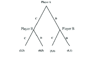
Figure 2-1: Prisoners’ Dilemma in extensive form

Both the sequential move game and simultaneous move game can be represented by extensive form. In the case of simultaneous move games either a dotted line or circle is drawn around two different vertices to show that they are the part of the same information set which means that the players do not know at which point they are.

2.3 Examples

In the following we give some examples of classical games that very often appear in the literature on game theory.

2.3.1 Matching Pennies

Matching pennies is a simple example from a class of zero sum games. In this game two players Alice and Bob show heads or tails from a coin. If both are heads or both are tails then Alice wins, otherwise Bob wins. The payoff matrix for this game is

$$\overset{\text{ \ \ \ \ \ \ \ \ \ \ \ \ \ \ \ \ \ \ \ }\begin{array}[]{c}\text{{\large Bob}}\\ \begin{array}[]{cc}H\text{ \ \ \ \ }&T\end{array}\end{array}}{\text{{\large Alice}}\begin{array}[]{c}H\\ T\end{array}\left[\begin{array}[]{cc}\left(1,-1\right)&\left(-1,1\right)\\ \left(-1,1\right)&\left(1,-1\right)\end{array}\right]}$$ (2.2)

2.3.2 Prisoners’ Dilemma 

This game starts with a story of two suspects, say Alice and Bob, who have committed a crime together. Now they are being interrogated in a separate cell. The two possible moves for each player are to cooperate ($C$) or to defect ($D$) without any communication between them according to the following payoff matrix

$$\text{{\large Alice }}\begin{array}[]{c}C\\ D\end{array}\overset{}{\overset{\begin{array}[]{c}\text{{\large Bob}}\\ \begin{array}[]{cc}C\text{ \ \ \ \ }&D\end{array}\end{array}}{\left[\begin{array}[]{cc}\left(3,3\right)&\left(0,5\right)\\ \left(5,0\right)&\left(1,1\right)\end{array}\right]}}.$$ (2.3)

 It is clear from the above payoff matrix that $D$ is the dominant strategy for both players. Therefore, rational reasoning forces each player to play $D$. Thus ($D,D$) results as the Nash equilibrium of this game with payoffs $(1,1),$ which is not Pareto Optimal. However, it was possible for the players to get higher payoffs if they would have played $C$ instead of $D$. This is the origin of dilemma in this game [44]. A generalized payoff matrix for Prisoners Dilemma is given as

$$\text{{\large Alice }}\begin{array}[]{c}C\\ D\end{array}\overset{}{\overset{\begin{array}[]{c}\text{{\large Bob}}\\ \begin{array}[]{cc}C\text{ \ \ \ \ }&D\end{array}\end{array}}{\left[\begin{array}[]{cc}\left(r,r\right)&\left(s,t\right)\\ \left(t,s\right)&\left(u,u\right)\end{array}\right]}},$$ (2.4)

where $t>r>u>s.$

The games like Prisoners’ Dilemma are important for the study of game theory for two reasons. First the payoff structure of this game is applicable to many different strategic situations arising in economics, social, political and biological competitions. Second the nature of equilibrium outcome is very strange. The players rational reasoning to maximize the payoffs gives them the payoff which is lower than they could have achieved if they used their dominated strategies. This particular feature of the game received much attention that how the players can achieve better payoffs [1].

2.3.3 Chicken Game

The payoff matrix for this game is

$$\text{{\large Alice }}\begin{array}[]{c}C\\ D\end{array}\overset{}{\overset{\begin{array}[]{c}\text{{\large Bob}}\\ \begin{array}[]{cc}C\text{ \ \ \ \ }&D\end{array}\end{array}}{\left[\begin{array}[]{cc}\left(3,3\right)&\left(1,4\right)\\ \left(4,1\right)&\left(0,0\right)\end{array}\right]}}.$$ (2.5)

In this game two players drove their cars straight towards each other. The first to swerve to avoid a collision is the loser (chicken) and the one who keeps on driving straight is the winner. There is no dominant strategy in this game. There are two Nash equilibria $CD$ and $DC,$ the former is preferred by Bob and the latter is preferred by Alice. The dilemma of this game is that the Pareto Optimal strategy $CC$ is not NE.

2.3.4 Battle of Sexes

In the usual exposition of this game two players Alice and Bob are trying to decide a place to spend Saturday evening. Alice wants to attend Opera while Bob is interested in watching TV at home and both would prefer to spend the evening together. The game is represented by the following payoff matrix:

$$\text{{\large Alice}}\overset{\begin{array}[]{c}\end{array}}{\begin{array}[]{c}O\\ T\end{array}}\overset{\begin{array}[]{c}\text{{\large Bob}}\\ \begin{array}[]{cc}\text{ }O\text{ \ \ \ \ \ \ }&T\end{array}\end{array}}{\left[\begin{array}[]{cc}(\alpha,\beta)&(\sigma,\sigma)\\ (\sigma,\sigma)&(\beta,\alpha)\end{array}\right],}$$ (2.6)

where $O$ and $T$ represent Opera and TV, respectively, and $\alpha$, $\beta$, $\sigma$ are the payoffs for players for different choices of strategies with $\alpha>\beta>\sigma$. There are two Nash equilibria $(O,O)$ and $(T,T)$ existing in the classical form of the game. In absence of any communication between Alice and Bob, there exists a dilemma as Nash equilibria $\left(O,O\right)$ suits Alice whereas Bob prefers $(T,T).$ As a result both players could end up with worst payoff in case they play mismatched strategies.

2.3.5 Rock-Scissors-Paper

In this game Alice and Bob make one of the symbols with their hand simultaneously, a rock, paper, scissors. In this game a player wins, loses or ties. The simple rule of the game is that paper covers rock so a player who makes the symbol of paper wins over the player who makes the symbol of rock. Scissors cuts paper so a player making the symbol of scissors win over the player making the symbol of paper. The rock breaks scissors therefore, the player who makes the symbol of rock wins over the player who makes scissors. If both make the same symbol then the game ties. The payoff matrix for this game is

$$\text{{\large Alice}}\overset{\begin{array}[]{c}\end{array}}{\begin{array}[]{c}R\\ S\\ P\end{array}}\overset{\overset{}{\begin{array}[]{c}\text{{\large Bob}}\\ \begin{array}[]{ccc}R&S&P\end{array}\end{array}}}{\left[\begin{array}[]{ccc}0&1&-1\\ -1&0&1\\ 1&-1&0\end{array}\right]}.$$ (2.7)

2.4 Applications of Game Theory

Game theory models the real life situations in an abstract manner. Due to their abstraction these models can be applied to study a wide range of phenomena [1, 41, 42, 45]. The best examples are the application of the theory of Nash equilibrium concept to study oligopolistic and political competitions, explanation of the distribution of tongue length in bees and tube length in flowers with the help of the theory of mixed strategy equilibrium, the use of the theory of repeated games in social phenomena like threats and promises [41]. Furthermore the models of game theory are successfully being used in fields including warfare, anthropology, social psychology, economics, politics, business, international relations, philosophy and biology. It is said that the importance of game theory for social sciences is the same as the importance of mathematics is for natural sciences [46]. Now there is an increasing interest of applying it to physics [8].

A. Dixit and S. Skeath [1] explained the role of games in real life as: Our life is full of events that resemble games. Many events and their outcomes around us force us to ask why did it happen like this? If we can find the decision makers involved in these situations who have different aims and interests then game theory provides us the answer. One of the interesting examples is the cutthroat competition in business where the rivals are trapped in Prisoners’ Dilemma like situation. Similarly in situations where multiple decision makers interact strategically, game theory can help to foresee the actions of rivals and the outcome of their actions. On the other hand we can provide services to a participant involved in any game like situation to advise him what strategies are good and which one leads to disaster.

Chapter 3 Review of Quantum Mechanics

Quantum mechanics is the mathematical theory for the description of nature. Its concepts are very different than those of classical physics. It was developed in response to the failure of classical physics to explain the atomic structure and some properties of electromagnetic radiations. Consequently there developed a theory that not only can explain the structure and the properties of the atoms and how they interact in molecules and solids but also the properties of subatomic particles such as protons and neutrons. In this chapter we explain some concepts of quantum mechanics. In preparation of this chapter we used the Refs. [22, 47].

3.1 Basic Concepts

A state is the complete description of the quantum system. For a physical state of a system it is a ray in Hilbert space.

3.1.1 Hilbert Space

The Hilbert space is specified by the following properties :

1. It is a vector space over the complex numbers $C$. In Dirac’s ket-bra notation the vectors are denoted by ket vectors $\left|\psi\right\rangle$.

2. It has an inner product $\left\langle\phi\right.\left|\psi\right\rangle$ that maps an ordered pair of vectors to $C$ defined by the following properties.

   1. Positivity: $\left\langle\psi\right.\left|\psi\right\rangle>0$ for $\left|\psi\right\rangle\neq 0$, where $\left\langle\psi\right|$ is called bra vector.

   2. Linearity: For any two vectors $\left|\psi_{1}\right\rangle,$ $\left|\psi_{2}\right\rangle$ and $\left|\phi\right\rangle$ we have

      $$\left\langle\phi\right|\left(a\left|\psi_{1}\right\rangle+b\left|\psi_{2}\right\rangle\right)=a\left\langle\phi\right.\left|\psi_{1}\right\rangle+b\left\langle\phi\right.\left|\psi_{2}\right\rangle.$$

   3. Skew symmetry: $\left\langle\phi\right.\left|\psi\right\rangle=\left\langle\psi\right.\left|\phi\right\rangle^{\ast}$ where $\ast$ denotes the complex conjugate.

3. It is complete in the norm $\left|\left|\psi\right|\right|=\left\langle\psi\right.\left|\psi\right\rangle^{\frac{1}{2}}$.

3.1.2 Observable

It is the physical property of quantum system that can be measured e.g. position, spin, and energy of a system. The observables are represented by Hermitian operators in the Hilbert space. Every observable $\hat{A}$ has a spectral decomposition of the form

$$\hat{A}=\underset{m}{\sum}\lambda_{m}\hat{P}_{m},$$ (3.1)

where $\hat{P}_{m}$ is the projector onto the eigen space of $\hat{A}$ with eigenvalue $\lambda_{m}.$

3.1.3 Pure State

A pure quantum state is the state that can be described by a ket vector. Mathematically it is written as

$$\left|\psi\right\rangle=\underset{i}{\sum}a_{i}\left|\psi_{i}\right\rangle,$$ (3.2)

where $a_{i}$ are complex numbers.

3.1.4 Mixed State

Mixed state is a statistical mixture of two or more pure states. For example

$$\rho=\frac{1}{2}\left|\psi\right\rangle\left\langle\psi\right|+\frac{1}{2}\left|\phi\right\rangle\left\langle\phi\right|,$$ (3.3)

is a mixed state where $\left|\psi\right\rangle$ and $\left|\phi\right\rangle$ are two pure states.

3.1.5 Density Matrix

A density matrix or density operator describes the statistical state of a quantum system. Its analogous concept in classical statistical mechanics is phase-space density which gives the probability distribution of position and momentum. The need for a statistical description via density matrices arises when it is not possible to describe a quantum mechanical system by states represented by ket vectors.

For any pure state density matrix is given by the projection operator of the state and for a mixed state it is the sum of projectors i.e.

$$\rho=\underset{i}{\sum}p_{i}\left|\psi_{i}\right\rangle\left\langle\psi_{i}\right|,$$ (3.4)

where $p_{i}$ is the probability of the system being in a quantum-mechanical state $\left|\psi_{i}\right\rangle.$ The expectation value of of any operator $\hat{M}$ can be found by density operator using the formula

$$M=\text{Tr}\left[\rho\hat{M}\right]=\underset{i}{\sum}p_{i}\left\langle\psi_{i}\right|\hat{M}\left|\psi_{i}\right\rangle,$$ (3.5)

where Tr represents the trace of a matrix. The probabilities $p_{i}$ are nonnegative numbers and normalized i.e. the sum of all the probabilities equals one. For the case of density matrix it is stated that $\rho$ is a positive semidefinite Hermitian operator and its trace is one i.e. its eigenvalues are nonnegative and sum to one.

3.1.6 Qubit

The unit of classical information is bit. A bit is indivisible and has only two possible values $0$ or $1$. The corresponding unit of quantum information is qubit or quantum bit. The simplest possible Hilbert state is two dimensional Hilbert space with orthonormal basis $\left|0\right\rangle$ and $\left|1\right\rangle.$ These basis correspond to classical bits $0$ and $1$. The difference between bits and qubits is that a qubit can also exist in a state other than $\left|0\right\rangle$ or $\left|1\right\rangle$ in the form of linear combination called superposition. Mathematically it is written as

$$\left|\psi\right\rangle=a\left|0\right\rangle+b\left|1\right\rangle,$$ (3.6)

when $a$ and $b$ are complex numbers with $\left|a\right|^{2}+\left|b\right|^{2}=1.$ If a measurement which distinguishes $\left|0\right\rangle$ from $\left|1\right\rangle$ is performed on this qubit then the outcome is $\left|0\right\rangle$ with probability $\left|a\right|^{2}$ and $\left|1\right\rangle$ with probability $\left|b\right|^{2}$. Furthermore except for the special cases $a=0$ or $b=0$ the measurement disturbs the state of a qubit. If a qubit is unknown then there is no way to determine $a$ and $b$ with single measurement. However with this measurement the qubit is prepared in known state $\left|0\right\rangle$ or $\left|1\right\rangle$ which is different from its initial form. The difference between the qubits and bits in this respect is that a classical bit can be measured without disturbing it and all the information that was encoded can be deciphered where as measurement disturbs the qubit. The physical quantities corresponding to the qubits $\left|0\right\rangle$ and $\left|1\right\rangle$ can be spin up and spin down state of an electron or the horizontal and vertical polarization of a photon respectively.

A geometrical representation which provides a useful means of visualizing the state of a single qubit is known as Bloch sphere representation as shown in figure 3-1.An arbitrary single qubit state can be written as

$$\left|\psi\right\rangle=e^{i\gamma}\left(\cos\frac{\theta}{2}\left|0\right\rangle+e^{i\phi}\sin\frac{\theta}{2}\left|1\right\rangle\right)$$ (3.7)

where $\theta,\phi$ and $\gamma$ are real numbers. The factor $e^{i\gamma}\$has no observable effects, therefore, it can be ignored. Furthermore $0\leq\theta\leq\pi$ and $0\leq\phi\leq 2\pi$ define a point on a unit three-dimensional sphere. In this representation the pure states lie on the surface of the sphere and the mixed states lie inside the sphere.

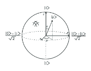
Figure 3-1: Bloch sphere representation of a qubit

3.2 Postulates of Quantum Mechanics

The formulation of quantum mechanics is based on the following postulates.

3.2.1 Postulate 1: State Space

The state of the system is completely described by a state vector which is a ray in Hilbert space. In Dirac ket-bra notation the states of the system are denoted by ket vectors $\left|\psi\right\rangle$. In this space the states $\left|\psi\right\rangle$ and $e^{i\alpha}\left|\psi\right\rangle$ describe the same physical state. For two given states $\left|\psi\right\rangle$ and $\left|\phi\right\rangle$ we can form another state by superposition as $a\left|\psi\right\rangle+b\left|\phi\right\rangle.$ The relative phase in this superposition state is physically significant, this means that $a\left|\psi\right\rangle+b\left|\phi\right\rangle$ is identical to $e^{i\alpha}\left(a\left|\psi\right\rangle+b\left|\phi\right\rangle\right)$ but different from $a\left|\psi\right\rangle+e^{i\alpha}b\left|\phi\right\rangle.$

3.2.2 Postulate 2: Evolution

The evolution of the state of a closed system is described by Schrodinger equation

$$i\hbar\frac{d\left|\psi\right\rangle}{dt}=\hat{H}\left|\psi\right\rangle,$$

where $\hbar$ is constant known as Planck’s constant and its value is determined experimentally. $\hat{H}$ is a Hermitian operator called the Hamiltonian of the system and it gives the energy of the system.

3.2.3 Postulate 3: Measurement

Quantum measurements are described by a collection $\left\{\hat{M}_{m}\right\}$ of measurement operators. These operators act on the state space of the system being measured. The index $m$ corresponds to one of the possible measurement outcomes. If the state of the quantum system is $\left|\psi\right\rangle$ immediately before the measurement then the probability that an outcome $m$ will occur is

$$p(m)=\left\langle\psi\right|\hat{M}_{m}^{\dagger}\hat{M}_{m}\left|\psi\right\rangle,$$ (3.8)

and the state of the system just after the measurement is

$$\left|\acute{\psi}\right\rangle=\frac{\hat{M}_{m}\left|\psi\right\rangle}{\sqrt{\left\langle\psi\right|\hat{M}_{m}^{\dagger}\hat{M}_{m}\left|\psi\right\rangle}}.$$ (3.9)

The measurement operators satisfy the completeness relation

$$\underset{m}{\sum}\hat{M}_{m}^{\dagger}\hat{M}_{m}=1,$$ (3.10)

which ensures the fact that probabilities sum to $1$.

There are two important special cases for the measurement process. One is the Projective measurement and the other is POVM (Positive Operator Value Measure).

Projective Measurement

In this case the measurement operators $\hat{M}$ in addition to completeness relation (3.10) also satisfy the condition that $\hat{M}_{m}$ are orthogonal projectors. Mathematically it can be written as

$$\hat{M}_{m^{{}^{\prime}}}\hat{M}_{m}=\delta_{m,m^{{}^{\prime}}}\hat{M}_{m}.$$ (3.11)

A projective measurement is described by a Hermitian operator $\hat{M}$ on the state space of the system. This Hermitian operator is termed as observable. The spectral decomposition of this observable is

$$\hat{M}=\underset{m}{\sum}mP_{m},$$ (3.12)

where $P_{m}$ is the projector onto the eigen space of $\hat{M}$ with eigenvalues $m$. On measuring the state $\left|\psi\right\rangle$ the probability of getting result $m$ is

$$p(m)=\left\langle\psi\right|P_{m}\left|\psi\right\rangle,$$ (3.13)

and the state of the system just after the measurement is

$$\left|\acute{\psi}\right\rangle=\frac{P_{m}\left|\psi\right\rangle}{\sqrt{\left\langle\psi\right|P_{m}\left|\psi\right\rangle}}.$$ (3.14)

If the system is subjected to same measurement immediately after the projective measurement the same outcome occurs with certainty.

POVM

In certain experiments the post measurement state of the system is of little interest whereas the main item of interest is the probabilities of the respective measurements. One of the examples of such experiment is the Stern Gerlach experiment. The mathematical tool for measurement in such a case is POVM. A POVM on quantum system is a collection, $\{\hat{E}_{m}\}$ of positive operators satisfying

$$\underset{m}{\sum}\hat{E}_{m}=I,$$ (3.15)

where $I$ is the identity operator. When a state $\left|\psi\right\rangle$ is subjected to POVM the probability of the outcome $m$ is

$$p(m)=\left\langle\psi\right|\hat{E}_{m}\left|\psi\right\rangle.$$ (3.16)

The state after measurement is not specified and therefore the measurement cannot be repeated.

3.2.4 Postulate 4 : Composite System

The state space of the composite physical system is the tensor product of the component systems. If we have a quantum mechanical system composed of $n$ quantum systems such that for each system $i$ the state is $\left|\psi_{i}\right\rangle.$ Then the joint state for the whole system is given as

$$\left|\Psi\right\rangle=\left|\psi_{1}\right\rangle\otimes\left|\psi_{2}\right\rangle\text{........}\otimes\left|\psi_{n}\right\rangle.$$ (3.17)

One of the interesting properties of the composite system which is unique to quantum system is entanglement.

Entanglement

The state of a composite quantum system can be written as a tensor product of its component system states. For example, the state of a system composed of two qubits is specified by a vector in a tensor product space spanned by the basis $\left|00\right\rangle,\left|01\right\rangle,\left|10\right\rangle,\left|11\right\rangle$. The quantum mechanical system can also exist as a linear combination or superposition of the states. Out of these states there exist some states in which there is a strong correlation between the components as compared to classical systems. These states are non-separable i.e. cannot be written as a product of the component systems. The state of a composite system that cannot be written as product of the states of its component systems is called entangled state. The well known examples of maximally entangled states are

$$\left|\psi^{+}\right\rangle = \frac{1}{\sqrt{2}}\left(\left|0_{A}0_{B}\right\rangle+\left|1_{A}1_{B}\right\rangle\right)$$ (3.18a)

$$\left|\psi^{-}\right\rangle = \frac{1}{\sqrt{2}}\left(\left|0_{A}0_{B}\right\rangle-\left|1_{A}1_{B}\right\rangle\right)$$ (3.18b)

$$\left|\phi^{+}\right\rangle = \frac{1}{\sqrt{2}}\left(\left|0_{A}1_{B}\right\rangle+\left|1_{A}0_{B}\right\rangle\right)$$ (3.18c)

$$\left|\phi^{-}\right\rangle = \frac{1}{\sqrt{2}}\left(\left|0_{A}1_{B}\right\rangle-\left|1_{A}0_{B}\right\rangle\right)$$ (3.18d)

where the first element in the ket refers to system A (first system) and the second to system B (second system). The states given by Eqs. (3.18) are known as Bell states. Note that none of these states can be written as the product of two states describing the state of the particles. Whenever measurement is performed on any member of the set then entanglement is destroyed and the particles obtain the definite state. In an entangled system the observables are strongly correlated hence required to be specified with reference to other objects even if they are far apart. For example for the Bell state

$$\left|\phi^{-}\right\rangle=\frac{1}{\sqrt{2}}\left(\left|0_{A}1_{B}\right\rangle-\left|1_{A}0_{B}\right\rangle\right)$$ (3.19)

it is impossible to attribute a definite state to either system for the two observers Alice and Bob observing the first and second system respectively. Alice performs measurement on first system in computational basis $\left|0\right\rangle$, $\left|1\right\rangle$. There are two outcomes which are equally likely (a) if Alice gets $\left|0\right\rangle$ then the system collapses to the state $\left|01\right\rangle$ and (b) if Alice gets $\left|1\right\rangle$ then the system collapses to $\left|10\right\rangle.$ For the first result of Alice any subsequent measurement by Bob always returns $\left|1\right\rangle$ and for the second result of Alice the subsequent measurement by Bob returns $\left|0\right\rangle$. It means that the measurement performed by Alice has changed the second system even if both the systems are spatially separated.

Chapter 4 Quantum Game Theory

In 1970’s Maynard Smith gave a new solution concept to game theory introducing the notion of evolutionary stable strategies (ESS) [48]. He assumed that a perfectly rational being is not a necessary element to recognize the best strategies in a game but each player participating in the game is hardwared or programmed in with a particular strategy by nature. When the game begins, the players contest with the players programmed with the same or some different strategies. The payoffs are rewarded to players against their strategies. The strategy that fares better, multiply faster and the worst strategy declines [1]. As a result only the strategies with best payoff sustain while the others are swept out. These techniques have successfully been used by biologists to model the behavior of animals and bacteria. Exploiting these techniques computer scientists developed some efficient algorithms for optimization problems known as genetic algorithms [49]. These algorithms are aimed to improve the understanding of natural adaptation process, and to design artificial systems having properties similar to natural systems [50]. On the other hand it has recently been shown that games are also being played at microscopic level by RNA virus [51]. Therefore, it will be very interesting to find whether the microscopic particles such as electrons or atoms are engaged in any type of quantum contest. One of the reasons behind these believes is that in some situations atoms and electrons have to choose between equally advantageous states that is a dilemma formally known as frustration [52]. It is expected that quantum games might help these frustrated atoms in resolving such dilemmas [53]. It is also believed that frustration is involved in the phenomenon like high temperature superconductivity. If it ever becomes possible to find the particle at play then quantum games might help to understand the phenomenon of high temperature superconductivity [53]. Quantum cloning and quantum state estimation has already been proved as games [14] and quantum cryptography is also a game played between the sender, the receiver and the spy [13]. These techniques of quantum cryptography might help constructing a quantum stock market where the traders would have the opportunity to encode their decisions in qubits. In such a market entanglement could be used as a helpful resource for traders to cooperate so that they could avoid crashes that is equivalent to the loss of everybody in game theory [53]. It is also expected that quantum games will help to introduce new business models for selling digital contents on internet that will discourage illegal downloading [54]. One of the interesting phenomena that has recently been discovered is Parrondo effect in which two losing games when combined have a tendency to win [55]. Classical Parrondo games and their relation to Brownian ratchet has also gained much interest [56, 57, 58, 59]. Parrondo games have been extended to quantum domain [60, 61]. A connection between Parrondo effects and the design of quantum algorithms has also been established [37, 62] and it is further expected that quantum Parrondo games can be helpful to control qubit decoherence [63]. A connection between quantum games and quantum algorithm for an oracle problem has been established as well [64]. Some search algorithms such as simulated annealing [65, 66] and adiabatic algorithms[67, 68] are also expected to be reformulated in the language of quantum games that might result in a strong connection between evolutionary games and games derived from the dynamics of physical systems [63]. Furthermore it is more efficient to play quantum games [69]. When we entangle two qubits shared between the players then the players have the greater number of strategies to choose from as compared to classical games. Therefore, less information needs to be exchanged in order to play the quantized versions of the classical games.

Quantum computation, quantum cryptography and quantum communication protocols are some prominent practical manifestations of quantum mechanics where the quantum description of the system has provided clear advantage over the classical counterparts. Simon’s quantum algorithm to identify the period of a function chosen by oracle [70], Shor’s polynomial time quantum algorithm [71] and the key distribution protocol given by Bennett and Brassard [98] and by Ekert [38] are some well known examples. Another amazing manifestation of quantum mechanical effects is superdense coding. Where using entanglement as a resource a sender can transmit two bits of classical information to a receiver by sending single qubit that is in her possession [22]. The clear superiority of the use of quantum mechanical resources in the above well established disciplines makes it natural to think about quantum strategies and quantum games that is, if the classical strategies of the players can be pure or mixed then why these cannot be entangled? Whether these entangled strategies can be helpful in resolving the dilemmas in classical games such as that in Prisoners’ Dilemma and the Battle of Sexes and whether there is any advantage in playing quantum strategies against classical strategies? Whether this new born field can be of any help in reformulating the protocols of quantum information theory and is capable of introducing new protocols and new algorithms? These are the questions mostly addressed in quantum game theory. In the following we explain the first quantum game that was originally introduced to demonstrate the advantage that quantum strategies can achieve over the classical ones.

4.1 Quantum Penny Flip Game

Quantum penny flip game [26] is the simplest example to demonstrate the advantage that a quantum player, Bob can have over a classical player, Alice. The framework of this game is as follows. Alice places a coin with head up state in a box. Bob is given the options either to flip the coin or to leave it unchanged. Then Alice takes her turn with the same options without having look at the coin. Finally, Bob takes his turn with the same options without looking at the coin. If at the end the coin is head up then Bob wins otherwise Alice wins.

This is an example of a zero sum game where the profit of one player means the loss of other player. The payoff matrix for this game is

$$\text{{\large Alice} }\begin{array}[]{c}N\\ F\end{array}\overset{}{\overset{\overset{}{\begin{array}[]{c}\text{{\large Bob}}\\ \begin{array}[]{cccc}NN&NF&FN&FF\end{array}\end{array}}}{\left[\begin{array}[]{cccc}-1&1&1&-1\\ 1&-1&-1&1\end{array}\right],}}$$ (4.1)

where $F$ stands for flipping and $N$ for not flipping the coin. According to classical game theory this game has no deterministic solution and deterministic Nash equilibrium [2, 3]. In other words, there exist no such pair of pure strategies from which unilateral withdrawal of a player can enhance his/her payoff. However, there exists a mixed strategies Nash equilibrium which is a pair of mixed strategies consisting of Alice flipping the coin with probability $\frac{1}{2}$ and Bob playing his strategies with probabilities $\frac{1}{4}$. When the game starts then to Alice surprise Bob, the quantum player, always wins. Quantum mechanics tells the entre nous that has blindsided Alice.

Quantum games are played using quantum objects. Therefore to see that how Bob can win we replace the classical coin with a quantum coin. The main difference between classical coin and quantum coin is that a classical coin can have one of two possible states i.e. either head or tail whereas a quantum coin can also exist in a state that is superposition of head and tail. In this way unlike a classical coin a quantum coin has infinite number of states. One of the very suitable examples of a quantum coin can be an electron defining head by the spin in +z-axis and tail by spin pointing along -z-axis. This coin is capable of having a linear combination of the head and tail states known as superposition in quantum mechanics. On the other hand Bob is also capable of playing quantum strategies that Alice has never heard before. These strategies are adept in placing the quantum coin in the superposition of head and tail states in the two dimensional Hilbert space. Let the head of the quantum coin be represented by $\left|0\right\rangle$ and tail by $\left|1\right\rangle$ in a 2-dimensional Hilbert space. The strategies of the players can be represented by $2\times 2$ matrices then the move $F$, to flip and the move $N$, not to flip the coin are of the form

$$F=\left[\begin{array}[]{cc}0&1\\ 1&0\end{array}\right],\text{ \ }N=\left[\begin{array}[]{cc}1&0\\ 0&1\end{array}\right].$$ (4.2)

When the game starts Alice places the coin in the head up state i.e. the initial state of coin is $\left|0\right\rangle$. Then Bob takes his turn and proceeds the game by applying the Hadamard gate

$$H=\frac{1}{\sqrt{2}}\left[\begin{array}[]{cc}1&1\\ 1&-1\end{array}\right],$$ (4.3)

that transforms the system to $\frac{1}{\sqrt{2}}\left(\left|0\right\rangle+\left|1\right\rangle\right)$ that is an equal mixture of the head and tail states. Now on her turn, Alice can either leave the coin as it is (apply $N)$ or flip the coin (apply $F$). If the coherence of the system is not effected by actions of Alice then clearly the state of the quantum system remains unaltered. Bob exploiting this fact again applies Hadamard gate while taking his turn and the final state of the system becomes $\left|0\right\rangle$ resulting a certain win for Bob.

The interesting episode in competition of Alice and Bob led many scientists to think about the quantization of non-zero sum games. In such games although the win of a player is not a loss of the other player yet the rational reasoning to enhance the payoffs can produce undesired outcomes. Taking an interesting example of such a game known as Prisoners’ Dilemma (see section 2.3), Eisert et al. [27] showed that the dilemma which exist in the classical version of the game does not exist in quantum version of this game. Further they succeeded in finding a quantum strategy which always wins over any classical strategy. Inspired by their work, Marinatto and Weber [28] proposed another interesting scheme to quantize the game of Battle of Sexes (see section 2.3). They introduced Hilbert structure to the strategic space of the game and argued that if the players are allowed to play quantum strategies involving unitary operators for maximally entangled initial state the game has a unique solution, and dilemma could be resolved.

In the following paragraphs we give a brief introduction to both these quantization schemes one by one.

4.2 Eisert, Wilkens and Lewenstein Quantization Scheme

Eisert et al. [27] introduced an elegant quantization scheme to help resolve the dilemma in an interesting game of Prisoners’ Dilemma with the payoff matrix of the form (2.3). This quantization scheme is a physical model which consists of the following elements known to both the players.

1. A source of producing two bits, one bit for each player.

2. Physical instruments that enables the player to manipulate their own bits in a strategic manner.

3. A physical measurement device which determines the players payoff from the strategically manipulated final state of two bits.

The classical strategies $C$ (Cooperate) and $D$ (Defect) are assigned two basis vectors $\left|C\right\rangle$ and $\left|D\right\rangle$ respectively, in a Hilbert space of a two level system. The state of the game at any instant is a vector in the tensor product space spanned by the basis vectors $\left|CC\right\rangle,\left|CD\right\rangle,\left|DC\right\rangle,\left|DD\right\rangle$ where the first entry in the ket refers to the Alice’s bit and the second entry is for Bob. The experimental setup for this quantization scheme is shown in figure 4-1.

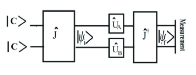
Figure 4-1: Eisert et al. quantization scheme.

The game starts with an initial entangled state $\left|\psi_{i}\right\rangle=\hat{J}\left|CC\right\rangle$ where $\hat{J}$ is a unitary operator that entangles the players qubits and it is known to both the players. The operator $\hat{J}$ is symmetric for fair games. The strategies of the players are the unitary operators

$$\hat{U}(\theta_{i},\phi_{i})=\left[\begin{array}[]{cc}e^{i\phi_{i}}\cos\frac{\theta_{i}}{2}&\sin\frac{\theta_{i}}{2}\\ -\sin\frac{\theta_{i}}{2}&e^{-i\phi_{i}}\cos\frac{\theta_{i}}{2}\end{array}\right],$$ (4.4)

with $0\leq\theta\leq\pi,0\leq\phi\leq\frac{\pi}{2}.$ The classical strategies to cooperate $\hat{C}=\hat{U}(0,0)$ and to defect $\hat{D}=\hat{U}(\pi,0)$. To ensure that the classical Prisoners’ Dilemma is the subset of its quantum version the following set of subsidiary conditions were imposed by Eisert et al.

$$\left[\hat{J},\hat{D}\otimes\hat{D}\right]=0,\left[\hat{J},\hat{C}\otimes\hat{D}\right]=0,\left[\hat{J},\hat{D}\otimes\hat{C}\right]=0,$$ (4.5)

From conditions (4.5) it comes out that

$$\hat{J}=\exp\left\{i\frac{\gamma}{2}\hat{D}\otimes\hat{D}\right\},$$ (4.6)

where $\gamma\in\left[0,\frac{\pi}{2}\right]$.

The strategic moves of Alice and Bob are the unitary operators $\hat{U}_{A}(\theta_{A},\phi_{A})$ and $\hat{U}_{B}(\theta_{B},\phi_{B})$ respectively. After the application of these strategies by players the state of the game evolves to

$$\left|\psi_{f_{0}}\right\rangle=\left(\hat{U}_{A}\otimes\hat{U}_{B}\right)\hat{J}\left|CC\right\rangle.$$ (4.7)

Prior to measurement for finding the payoffs of the players a reversible two-bit gate $\hat{J}^{\dagger}$ is applied and the state of the game becomes

$$\left|\psi_{f}\right\rangle=\hat{J}^{\dagger}\left(\hat{U}_{A}\otimes\hat{U}_{B}\right)\hat{J}\left|CC\right\rangle.$$ (4.8)

This follows a pair of Stern-Gerlach type detectors for measurement and the expected payoff of Alice comes out to be

$$\$_{A}=\left[\$_{CC}\right]_{A,B}\left|\left\langle CC\right.\left|\psi_{f}\right\rangle\right|^{2}+\left[\$_{DD}\right]_{A,B}\left|\left\langle DD\right.\left|\psi_{f}\right\rangle\right|^{2}+\left[\$_{DC}\right]_{A,B}\left|\left\langle DC\right.\left|\psi_{f}\right\rangle\right|^{2}+\left[\$_{CD}\right]_{A,B}\left|\left\langle CD\right.\left|\psi_{f}\right\rangle\right|^{2},$$ (4.9)

Here it is important to note that Alice’s payoffs $\$_{A}$ depends on the strategy $\hat{U}_{A}(\theta_{A},\phi_{A})$ of Alice as well as on the Bob’s strategy $\hat{U}_{B}(\theta_{B},\phi_{B}).$

In terms of density matrices the initial state $\rho_{i}=\left|\psi_{i}\right\rangle\left\langle\psi_{i}\right|$ after the actions of the players transform to

$$\rho_{f}=\left(\hat{U}_{A}\otimes\hat{U}_{B}\right)\rho_{i}\left(\hat{U}_{A}\otimes\hat{U}_{B}\right)^{\dagger}.$$ (4.10)

To perform measurement arbiter uses the following payoff operators

$$\pi_{CC} = \left|\psi_{CC}\right\rangle\left\langle\psi_{CC}\right|,\text{ \ \ }\left|\psi_{CC}\right\rangle=\frac{\left|CC\right\rangle+i\left|DD\right\rangle}{\sqrt{2}},$$

$$\pi_{CD} = \left|\psi_{CD}\right\rangle\left\langle\psi_{CD}\right|,\text{ \ \ }\left|\psi_{CD}\right\rangle=\frac{\left|CD\right\rangle-i\left|CD\right\rangle}{\sqrt{2}},$$

$$\pi_{DC} = \left|\psi_{DC}\right\rangle\left\langle\psi_{DC}\right|,\text{ \ \ }\left|\psi_{DC}\right\rangle=\frac{\left|DC\right\rangle-i\left|CD\right\rangle}{\sqrt{2}}$$

$$\pi_{DD} = \left|\psi_{DD}\right\rangle\left\langle\psi_{DD}\right|,\text{ \ \ }\left|\psi_{DD}\right\rangle=\frac{\left|DD\right\rangle+i\left|CC\right\rangle}{\sqrt{2}},$$ (4.11)

and the expected payoffs for Alice and Bob are computed as

$$\$_{A,B}=\left[\$_{CC}\right]_{A,B}Tr\left[\pi_{CC}\rho_{f}\right]+\left[\$_{CD}\right]_{A,B}Tr\left[\pi_{CD}\rho_{f}\right]+\left[\$_{DC}\right]_{A,B}Tr\left[\pi_{DC}\rho_{f}\right]+\left[\$_{DD}\right]_{A,B}Tr\left[\pi_{DD}\rho_{f}\right],$$ (4.12)

where $\left[\$_{ij}\right]_{A,B}$ are the elements of the payoff matrix for Alice and Bob. Eisert et al. [27] analyzed Prisoners’ Dilemma game under one and two parameters set of strategies [72] using the payoff matrix (2.3) as follows

4.2.1 One Parameter Set of Strategies.

In the one parameter set of strategies the players are restricted to apply the local operators of the form

$$\hat{U}(\theta_{i})=\left[\begin{array}[]{cc}\cos\frac{\theta_{i}}{2}&\sin\frac{\theta_{i}}{2}\\ -\sin\frac{\theta_{i}}{2}&\cos\frac{\theta_{i}}{2}\end{array}\right],$$ (4.13)

here $0\leq\theta\leq\pi$ and $i=1,2$. For maximally entangled initial state

$$\left|\psi_{CC}\right\rangle=\hat{J}\left|CC\right\rangle=\frac{\left|CC\right\rangle+i\left|DD\right\rangle}{\sqrt{2}},$$ (4.14)

by the use of Eq. (4.10), (4.11) and (4.12) the payoffs of the players become

$$\$_{A}(\theta_{1},\theta_{2}) = 3\left|\cos\frac{\theta_{1}}{2}\cos\frac{\theta_{2}}{2}\right|^{2}+5\left|\sin\frac{\theta_{1}}{2}\cos\frac{\theta_{2}}{2}\right|^{2}+\left|\sin\frac{\theta_{1}}{2}\sin\frac{\theta_{2}}{2}\right|^{2},$$ (4.15a)

$$\$_{B}(\theta_{1},\theta_{2}) = 3\left|\cos\frac{\theta_{1}}{2}\cos\frac{\theta_{2}}{2}\right|^{2}+5\left|\cos\frac{\theta_{1}}{2}\sin\frac{\theta_{2}}{2}\right|^{2}+\left|\sin\frac{\theta_{1}}{2}\sin\frac{\theta_{2}}{2}\right|^{2}.$$ (4.15b)

These payoffs are just like the payoffs of ordinary Prisoners’ Dilemma when the players are playing the classical strategies of cooperation with probabilities $$\cos^{2}\frac{\theta_{1}}{2} \cos^{2}\frac{\theta_{2}}{2}.$$ and The inequalities

$$\$_{A}(\pi,\theta_{2}) \geq \$_{A}(\theta_{1},\theta_{2}),$$

$$\$_{B}(\theta_{1},\pi) \geq \$_{B}(\theta_{1},\theta_{2}),$$ (4.16)

hold for all values of $\theta_{1}$ and $\theta_{2},$ giving $(D,D)$ as the Nash equilibrium of the game. However this Nash equilibrium is not Pareto Optimal as it is far from being efficient since $\$_{A}(\pi,\pi)=\$_{B}(\pi,\pi)=1,$ just like the classical  version of the game. Therefore, the one parameter set of strategies do not resolve the dilemma.

4.2.2 Two Parameter Set of Strategies

When the players are allowed to apply their local operators with two variable $\left(\theta,\phi\right)$ two parameters set of strategies results and their mathematical form is

$$\hat{U}(\theta_{i},\phi_{i})=\left[\begin{array}[]{cc}e^{i\phi_{i}}\cos\frac{\theta_{i}}{2}&\sin\frac{\theta_{i}}{2}\\ -\sin\frac{\theta_{i}}{2}&e^{-i\phi_{i}}\cos\frac{\theta_{i}}{2}\end{array}\right],$$ (4.17)

where $i=1,2.$ Using the Eq. (4.10), (4.11) and (4.12) the payoffs come out to be

$$\$_{A}\left(\theta_{1},\phi_{1},\theta_{2},\phi_{2}\right) =3\left|\cos\frac{\theta_{1}}{2}\cos\frac{\theta_{2}}{2}\cos\left(\phi_{1}+\phi_{2}\right)\right|^{2}$$

$$+\left|\cos\frac{\theta_{1}}{2}\cos\frac{\theta_{2}}{2}\sin\left(\phi_{1}+\phi_{2}\right)+\sin\frac{\theta_{1}}{2}\sin\frac{\theta_{2}}{2}\right|^{2}$$

$$+5\left|\sin\frac{\theta_{1}}{2}\cos\frac{\theta_{2}}{2}\cos\phi_{2}-\cos\frac{\theta_{1}}{2}\sin\frac{\theta_{2}}{2}\sin\phi_{1}\right|^{2},$$ (4.18)

$$\$_{B}\left(\theta_{1},\phi_{1},\theta_{2},\phi_{2}\right) = 3\left|\cos\frac{1}{2}\theta_{1}\cos\frac{1}{2}\theta_{2}\cos\left(\phi_{1}+\phi_{2}\right)\right|^{2}$$ (4.19)

$$+5\left|\cos\frac{1}{2}\theta_{1}\sin\frac{1}{2}\theta_{2}\cos\phi_{1}-\sin\frac{1}{2}\theta_{1}\cos\frac{1}{2}\theta_{2}\sin\phi_{2}\right|^{2}$$

$$+\left|\cos\frac{1}{2}\theta_{1}\cos\frac{1}{2}\theta_{2}\sin\left(\phi_{1}+\phi_{2}\right)+\sin\frac{1}{2}\theta_{1}\sin\frac{1}{2}\theta_{2}\right|^{2}.$$

In this case the Nash equilibrium $\left(\hat{D}\otimes\hat{D}\right)$ no more remains the Nash equilibrium of the game. However, there appears a new Nash Equilibrium $\left(\hat{Q}\otimes\hat{Q}\right)$ where

$$\hat{Q}=U(0,\frac{\pi}{2})=\left[\begin{array}[]{cc}i&0\\ 0&-i\end{array}\right].$$ (4.20)

Eisert et al. [27] argued that this unique Nash Equilibrium is Pareto Optimal with $\$_{A}(\hat{Q},\hat{Q})=\$_{B}(\hat{Q},\hat{Q})=3.$ They further pointed out that the dilemma in the classical version of game is no more present in the quantum form of the game.

4.2.3 The Miracle Move

Imagine a situation where one of the players say Alice has the access to whole of the strategic space where as Bob is restricted to apply classical strategies only i.e. $\phi_{B}=0$. In this case Eisert et al. [27] pointed out that for Prisoners’ Dilemma the quantum player Alice is always equipped with a strategy $\hat{M}(\theta,\phi)$ that gives her a sure success against the classical player, Bob. This quantum move $\hat{M}(\theta,\phi)$ is also known as Eisert miracle move and is given by

$$\hat{M}(\frac{\pi}{2},\frac{\pi}{2})=\frac{1}{\sqrt{2}}\left[\begin{array}[]{cc}i&1\\ -1&-i\end{array}\right].$$ (4.21)

The payoffs for Alice and Bob, when Alice is playing $\hat{M}(\frac{\pi}{2},\frac{\pi}{2})$ and Bob is playing any classical strategy $\hat{U}(\theta),$ are

$$\$_{A} = 3+2\sin\theta,$$

$$\$_{B} = \frac{\left(1-\sin\theta\right)}{2}.$$ (4.22)

It is clear from Eqs. (4.22) that a quantum player can outperform a classical player for all values of $\theta$. Furthermore it has also been shown that in this unfair game the payoff for quantum player is monotonically increasing function of $\gamma,$ the entanglement measure of the initial state $\left|\psi_{i}\right\rangle$ [33, 73]. For $\ \gamma=0,$ $D$ is the dominant strategy and the payoff of minimum value $1$ is achieved however at $\gamma=\frac{\pi}{2}$ the quantum player achieves the maximum advantage of $3$. Furthermore there exists a threshold value $\gamma_{th}=0.464$ below which Alice could not deviate form strategy $D.$ However beyond this threshold value she will discontinuously have to deviate from $D$ to $Q.$ At critical value of entanglement parameter there is a phase like transition between the classical and quantum domains of the game [33, 73]. 

4.2.4 Extension to Three Parameters Set of Strategies

In the Eisert et al. [27] scheme there seems no apparent reason for imposing a restriction on players to apply only to two parameters set of strategies. Although this set of strategies is not closed under composition yet it did not prevent many authors to investigate about the quantum games using this quantization scheme [73, 74, 75, 76].

Its extension to three parameters set of strategies can be accomplished using the operators of the form

$$\hat{U}(\theta,\phi,\psi)=\left[\begin{array}[]{cc}e^{i\phi}\cos\frac{\theta}{2}&ie^{i\psi}\sin\frac{\theta}{2}\\ ie^{-i\psi}\sin\frac{\theta}{2}&e^{-i\phi}\cos\frac{\theta}{2}\end{array}\right],$$ (4.23)

where $0\leq\theta\leq\pi,-\pi\leq\phi,\psi\leq\pi.$ In the case when the players have access to full strategy space as given in (4.23) then for every strategy of first player Alice the second player Bob also has a counter strategy as a result there is no pure strategies Nash equilibrium [77]. However, there can be mixed strategies (non-unique) Nash equilibrium [72].

4.2.5 Applications

An experimental demonstration of Eisert et al. [27] quantization scheme for Prisoners’ Dilemma game has been achieved on a two qubit nuclear magnetic resonance (NMR) computer with full range of entanglement parameter $\gamma$ ranging from $0$ to $\frac{\pi}{2}$ [78]. It is interesting to note that these results are in good agreement with theory. Such a type of demonstration has also been proposed on the optical computer [79]. Some other interesting issues that have been analyzed using this quantization scheme are, the proof of quantum Nash equilibrium theorem [37], evolutionarily stable strategies (ESS) [30], quantum verses classical player [80, 81, 82], the difference between classical and quantum correlations [75, 76] and the model of decoherence in the quantum games [127, 83]. In this model an increase in the amount of decoherence degrades the advantage of a quantum player over a classical player. However this advantage does not entirely disappear until the decoherence is maximum. Eisert et al. scheme can easily be implemented to all kinds of $2\times 2$ games. A possible classification of $2\times 2$ games has also been given by Huertas-Rosero [34].

4.2.6 Comments of Enk and Pike

Enk and Pike [84] argued that the solutions of Prisoners’ Dilemma as found by Eisert et. al [27] are neither quantum mechanical nor they solve classical game. But it can be generated by extending the classical payoff matrix of the game in such a way that it includes a pure strategy corresponding to $\hat{Q}$. They added that as if the quantum situation pointed out by Eisert et al. can be found classically then the only defence for quantum solution is its efficiency and it does not play any role in Prisoners’ Dilemma game. They also gave the suggestion to investigate the quantum games by exploiting the non-classical correlations in entangled states.

4.3 Marinatto and Weber Quantization Scheme

Marinatto and Weber [28] gave another interesting scheme for the quantization of non-zero sum games by taking an example of a famous game known as Battle of Sexes with the payoff matrix as in (2.6). To analyze this game in quantum domain Marinatto and Weber [28] gave Hilbert structure to the strategic space of the game by allowing the linear combinations of classical strategies. At the beginning of the game arbiter prepares two qubits quantum state and sends one qubit to each player. The players apply their tactics i.e. their local operators on the respective qubits and send them back to arbiter. The players’ tactics in this scheme are combinations of the identity operator $\hat{I}$ and the flip operator $\hat{C}$, with classical probabilities $p$ and $\left(1-p\right)$, respectively for Alice and $q$ and $\left(1-q\right)$ for Bob. This quantization scheme is depicted in fig. (4-2)

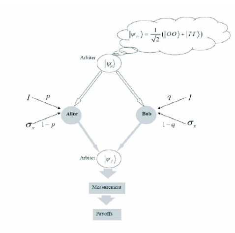
Figure 4-2: Marinatto and Weber quantization scheme. At the beginning of the game arbiter prepares two qubits entangled state $\left|\psi\right\rangle_{in}$ and sends one qubit to each player. The players apply their tactics i.e their local operators on their qubits and send back to arbiter. The players’ tactics in this scheme are combinations of the identity operator $I$ and the flip operator $C$, with classical probabilities $p$ and $\left(1-p\right)$, respectively for Alice and $q$ and $\left(1-q\right)$ for Bob.

Marinatto and Weber [28] supposed that the game starts from the initial state of the form

$$\left|\psi\right\rangle_{in}=a\left|OO\right\rangle+b\left|TT\right\rangle,\text{ \ \ }$$

$$\text{\ }\left|\text{\ }a\right|^{2}+\text{\ }\left|b\right|^{2}=1.$$ (4.24)

Here the first entry in ket-bra $\left|{}\right\rangle$ is for Alice and the second for Bob’s strategy and $O$ represents opera and $T$ represents TV (see 2.3.4). The density matrix for the quantum state 4.24 is defined by $\rho_{in}=\left|\psi_{in}\right\rangle\left\langle\psi_{in}\right|$ and takes the form

$$\rho_{in}=\left|a\right|^{2}\left|OO\right\rangle\left\langle OO\right|+ab^{\ast}\left|OO\right\rangle\left\langle TT\right|+a^{\ast}b\left|TT\right\rangle\left\langle OO\right|+\left|b\right|^{2}\left|TT\right\rangle\left\langle TT\right|.$$ (4.25)

The unitary operators $\hat{I}$ and $\hat{C}$  transform the strategy vectors $\left|O\right\rangle$ and $\left|T\right\rangle$ as follows

$$\hat{C}\left|O\right\rangle=\left|T\right\rangle,\text{ \ \ }\hat{C}\left|T\right\rangle=\left|O\right\rangle,\text{ \ \ }\hat{C}=\hat{C}^{\dagger}=\hat{C}^{-1}.$$ (4.26)

After the application of the tactics $\hat{I}$ and $\hat{C}$ with probability $p$ and $1-p$ respectively by Alice and with probabilities $q$ and $1-q$ by Bob respectively, the Eq. (4.25) becomes

$$\rho_{f}=pq\hat{I}_{A}\otimes\hat{I}_{B}\rho_{\hat{I}n}\hat{I}_{A}^{\dagger}\otimes\hat{I}_{B}^{\dagger}+p(1-q)\hat{I}_{A}\otimes\hat{C}_{B}\rho_{\hat{I}n}\hat{I}_{A}^{\dagger}\otimes\hat{C}_{B}^{\dagger}$$

$$+q(1-p)\hat{C}_{A}\otimes\hat{I}_{B}\rho_{\hat{I}n}\hat{C}_{A}^{\dagger}\otimes\hat{I}_{B}^{\dagger}+(1-p)(1-q)\hat{C}_{A}\otimes\hat{C}_{B}\rho_{\hat{I}n}\hat{C}_{A}^{\dagger}\otimes\hat{C}_{B}^{\dagger}.$$ (4.27)

Marinatto and Weber [28] defined the payoff operators for Alice and Bob as

$$P_{A} = \alpha\left|OO\right\rangle\left\langle OO\right|+\beta\left|TT\right\rangle\left\langle TT\right|+\sigma(\left|OT\right\rangle\left\langle OT\right|+\left|TO\right\rangle\left\langle TO\right|),$$

$$P_{B} = \beta\left|OO\right\rangle\left\langle OO\right|+\alpha\left|TT\right\rangle\left\langle TT\right|+\sigma(\left|OT\right\rangle\left\langle OT\right|+\left|TO\right\rangle\left\langle TO\right|),$$ (4.28)

and payoff functions are obtained as the mean values of these operators, i.e.,

$$\$_{A}(p,q)=\text{Tr}(P_{A}\rho_{f}),\text{ \ \ \ \ and\ \ \ \ \ }\$_{B}(p,q)=\text{Tr}(P_{B}\rho_{f}),$$ (4.29)

where Tr represents the trace. With the help of Eqs. (4.27), (4.28) and (4.29) the payoffs obtained for the players are

$$\$_{A}(p,q) = p\left[q\left(\alpha+\beta-2\sigma\right)-\alpha\left|b\right|^{2}-\beta\left|a\right|^{2}+\sigma\right]+$$ (4.30)

$$q\left[-\alpha\left|b\right|^{2}-\beta\left|a\right|^{2}+\sigma\right]+\alpha\left|b\right|^{2}+\beta\left|a\right|^{2},$$

$$\$_{B}(p,q) = q\left[p\left(\alpha+\beta-2\sigma\right)-\beta\left|b\right|^{2}-\alpha\left|a\right|^{2}+\sigma\right]+$$ (4.31)

$$p\left[-\beta\left|b\right|^{2}-\alpha\left|a\right|^{2}+\sigma\right]+\beta\left|b\right|^{2}+\alpha\left|a\right|^{2}.$$

The payoffs of both players also depend on the tactics/ strategy played by the other player. This is the explicit nature of the game. In the next we explore the Nash equilibria as found by Marinatto and Weber [28].

Let $\left(p^{\ast},q^{\ast}\right)$ be the Nash equilibrium (NE) of this game, then from the definition of the Nash equilibrium it is clear that

$$\$_{A}(p^{\ast},q^{\ast})-\$_{A}(p,q^{\ast}) = \left(p^{\ast}-p\right)\left[q^{\ast}\left(\alpha+\beta-2\sigma\right)-\alpha\left|b\right|^{2}-\beta\left|a\right|^{2}+\sigma\right]\geq 0,$$

$$\$_{B}(p^{\ast},q^{\ast})-\$_{B}(p^{\ast},q) = \left(q^{\ast}-q\right)\left[p^{\ast}\left(\alpha+\beta-2\sigma\right)-\beta\left|b\right|^{2}-\alpha\left|a\right|^{2}+\sigma\right]\geq 0.$$

For the inequalities (LABEL:NE-BoS) to hold it is necessary for both the expression in the parenthesis to be of the same sign. This gives rise to the following cases of interest.

Case (1)  When $p^{\ast}=q^{\ast}=1$ then the inequalities (LABEL:NE-BoS) hold if

$$\alpha\left|a\right|^{2}+\beta\left|b\right|^{2}-\sigma > 0,$$

$$\beta\left|a\right|^{2}+\alpha\left|b\right|^{2}-\sigma > 0.$$ (4.33)

The above conditions are satisfied for all values of $\left|a\right|^{2}$ and $\left|b\right|^{2}$ therefore, from Eqs. (4.30) and (4.31) the payoffs of the players become

$$\$_{A}(1,1) = \alpha\left|a\right|^{2}+\beta\left|b\right|^{2},$$

$$\$_{B}(1,1) = \beta\left|a\right|^{2}+\alpha\left|b\right|^{2}.$$ (4.34)

Case (2)  When $p^{\ast}=q^{\ast}=0$ then the inequalities (LABEL:NE-BoS) hold if

$$\alpha\left|b\right|^{2}+\beta\left|a\right|^{2}-\sigma > 0,$$

$$\beta\left|b\right|^{2}+\alpha\left|a\right|^{2}-\sigma > 0.$$ (4.35)

The above conditions are also satisfied for all values of $\left|a\right|^{2}$ and $\left|b\right|^{2}$ therefore, from Eqs. (4.30) and (4.31) the payoffs for the players are

$$\$_{A}(0,0) = \alpha\left|b\right|^{2}+\beta\left|a\right|^{2},$$

$$\$_{B}(0,0) = \beta\left|b\right|^{2}+\alpha\left|a\right|^{2}.$$ (4.36)

Case (3)  When $\acute{p}^{\ast}=\frac{\left(\beta-\sigma\right)\left|b\right|^{2}+\left(\alpha-\sigma\right)\left|a\right|^{2}}{\alpha+\beta-2\sigma},\acute{q}^{\ast}=\frac{\left(\alpha-\sigma\right)\left|b\right|^{2}+\left(\beta-\sigma\right)\left|a\right|^{2}}{\alpha+\beta-2\sigma}$ then due to the condition $\alpha>\beta>\sigma$ we see that $0<\acute{p}^{\ast}<1$ and $0<\acute{q}^{\ast}<1$ and hence from Eqs. (4.30) and (4.31) the payoffs for players become

$$\$_{A}\left(\acute{p}^{\ast},\acute{q}^{\ast}\right)=\$_{B}\left(\acute{p}^{\ast},\acute{q}^{\ast}\right)=\frac{\alpha\beta+\left(\alpha-\beta\right)^{2}\left|a\right|^{2}\left|b\right|^{2}-\sigma^{2}}{\alpha+\beta-2\sigma}.$$ (4.37)

It is clear from Eqs. (4.34), (4.36) and (4.37) that both the players will prefer to play strategies $p^{\ast}=q^{\ast}=1$ or $p^{\ast}=q^{\ast}=0$ rather than $\left(\acute{p}^{\ast},\acute{q}^{\ast}\right)$. But again they are unable to decide which of the two Nash equilibria they choose to play. It looks as if the dilemma is still there. However this dilemma can be resolved by comparing the payoffs of the players at these Nash equilibria. By the use of Eqs. (4.34) and (4.36) one gets

$$\$_{A}(1,1)-\$_{A}(0,0) = \left(\alpha-\beta\right)\left(\left|a\right|^{2}-\left|b\right|^{2}\right),$$

$$\$_{B}(1,1)-\$_{B}(0,0) = \left(\alpha-\beta\right)\left(\left|b\right|^{2}-\left|a\right|^{2}\right).$$ (4.38)

It is evident from Eq. (4.38) that for $\left|a\right|^{2}>\left|b\right|^{2}$ Alice would prefer the Nash equilibrium $\left(\ p^{\ast}=q^{\ast}=1\right)$ whereas Bob will prefer $\left(p^{\ast}=q^{\ast}=0\right)$, but for $\left|a\right|^{2}<\left|b\right|^{2}$ the choices of the players are interchanged. This gives a clue for the resolution of the dilemma. If the initial quantum state parameters are chosen as$\ \left|a\right|^{2}=\left|b\right|^{2}$ $=\frac{1}{2}$ then Eq. (4.24) gives

$$\left|\psi\right\rangle_{in}=\frac{\left|OO\right\rangle+\left|TT\right\rangle}{\sqrt{2}},$$ (4.39)

and by the use of Eq. (4.38) the payoffs become

$$\$_{A}=\$_{B}=\frac{\alpha+\beta}{2}.$$ (4.40)

These payoffs for both the players are same irrespective of the choice of $p^{\ast}=q^{\ast}=0$ or $p^{\ast}=q^{\ast}=1.$

On the other hand for mixed strategies ( $\acute{p}^{\ast}=\acute{q}^{\ast}=\frac{1}{2}$) the payoffs of the players for maximally entangled initial quantum state (4.39) with the help of Eq. (4.37) come out to be

$$\$_{A}=\$_{B}=\frac{\alpha+\beta+2\sigma}{4}.$$ (4.41)

Comparing Eqs. (4.40) and (4.41) it is clear that initial quantum state given by Eq. (4.39) which is maximally entangled state satisfies the Nash equilibrium conditions i.e. it is a best rational choice which is stable against unilateral deviation and it also gives higher reward then mixed strategy Nash Equilibrium at $\acute{p}^{\ast}=\acute{q}^{\ast}=\frac{1}{2}$. Marinatto and Weber [28] argued that this proves that maximally entangled strategy Eq. (4.39) used as initial quantum state resolves the dilemma present in the classical version of the Battle of Sexes.

4.3.1 Applications

This quantization scheme has widely been used in various context for the quantization of games. It gave very interesting results while investigating evolutionarily stable strategies (ESS) [30] and in the analysis of repeated games [32] etc. This quantization scheme has also been cast in a different manner where the players manipulate their strategies by the application of linear combination of the operators $\hat{I}$ and $\hat{C}$ as

$$\hat{O}=\sqrt{p}\hat{I}+\sqrt{1-p}\hat{C}.$$ (4.42)

The operator $\hat{O}$ is termed as quantum superposed operator (QSO) [85]. The explanation for this approach is based on the argument that each player is given a handle that can be moved continuously between $0$ and $1$. When the handle is set to $1$ it performs the $I$ operation, when set to $0$ it performs $\sigma_{x}$ operation and at position $1-p$ it performs the operation $\hat{O}=$ $\sqrt{p}\hat{I}+\sqrt{1-p}\hat{C}$.

4.3.2 Benjamin’s Comments

In an interesting comment Benjamin [77] pointed out that the dilemma is still there as the same payoff for the two Nash equilibria make them equally acceptable to the players and there is no way for the players to prefer “$1$” over “$0$”. In the absence of any communication between them they could end up with a situation $\left(1,0\right)$ or $\left(0,1\right)$ which corresponds to the worst payoff for both players. Benjamin argued that this is somewhat similar dilemma faced by players in classical version of the game.

4.3.3 Marinatto and Weber’s Reply

In their response to Benjamin’s comment, Marinatto and Weber [86] insisted that since both the NE $\left(0,0\right)$ and $\left(1,1\right)$ render the initial quantum state unchanged and corresponds to equal and maximum payoff for both the players, therefore, both of them would prefer $\left(1,1\right),$ as by choosing $p$ or $q$ equal to zero there is a danger for both the payers to get in to a situation $\left(1,0\right)$ or $\left(0,1\right)$ which corresponds to the lowest payoff.

In the next section we show that the worst case payoff scenario as pointed out by Benjamin is not due to the quantization scheme itself but it is due to the restriction imposed on initial quantum state parameters. If the game is allowed to start from more general quantum state then the conditions on the initial quantum state parameters can be set so that the payoffs for mismatched or worst case situations are different for different players which results into a unique solution of the game.

4.4 Resolution of Dilemma in Quantum Battle of Sexes.

In this section we analyze the game of quantum Battle of Sexes using the approach developed by Marinatto and Weber [28]. Instead of restricting to maximally entangled initial quantum state we consider a general initial quantum state. Exploiting the additional parameters in the initial state we present a condition for which unique solution of the game can be obtained. In particular we address the issues pointed out by Benjamin [39] in Marinatto and Weber [28] quantum version of the Battle of sexes game. In our approach, difference in the payoffs for the two players corresponding to so called worst-case situation leads to a unique solution of the game. The results reduce to that of Marinatto and Weber under appropriate conditions. It is further shown that initial state parameters can be controlled to make any possible pure strategy pair in the game to be Nash Equilibria and a unique solution of the game as well. However then it would not be interesting to draw a comparison with the classical version of the game.

Since for choosing strategy on the basis of Marinatto and Weber’s argument it requires complete information on the initial quantum state and in quantum games players are not supposed to measure the initial quantum state as initial quantum state is only used to communicate their choice of local operators to the arbiter [30, 37, 87]. The choice of these operators depend on the payoff matrix known to them. If, however a general initial quantum state is considered then a condition on the parameters of the initial quantum state can be obtained for which classical dilemma can be resolved and a unique solution of the quantum Battle of Sexes is achieved. In comparison to Marinatto and Weber [28] approach a condition can also be imposed for which payoffs corresponding to “mismatched or worst case situation” are different for two players which leads to a unique solution of the game. Since in quantum version of the game both players, Alice and Bob, apply their respective strategies to the initial quantum state given to them on the basis of payoff matrix given to them. In this approach the payoff matrix depends on the initial state and can be controlled by its parameters. Therefore the choice of general initial quantum state provides with additional parameters to control in comparison with Marinatto and Weber’s [28].

Let Alice and Bob have the following initial entangled state at their disposal

$$\left|\psi_{in}\right\rangle=a\left|OO\right\rangle+b\left|OT\right\rangle+c\left|TO\right\rangle+d\left|TT\right\rangle,$$ (4.43)

where  $\left|a\right|^{2}+\left|b\right|^{2}+\left|c\right|^{2}+\left|d\right|^{2}=1.$ Here the first entry in ket $\left|{}\right\rangle$ is for Alice and the second for Bob’s strategy. For $b$ and $c$ equal to zero Eq. (4.43) reduces to the initial maximally entangled quantum state used by Marinatto and Weber [28]. The unitary operators on the disposal of the players are defined as

$$\hat{C}\left|O\right\rangle=\left|T\right\rangle,\text{ \ \ }\hat{C}\left|T\right\rangle=\left|O\right\rangle,\text{ \ \ }\hat{C}=\hat{C}^{\dagger}=\hat{C}^{-1}.$$ (4.44)

Following the Marinatto and Weber, take $p\hat{I}+(1-p)\hat{C}$ and $q\hat{I}+(1-q)\hat{C}$ as the strategies for the two players, respectively, with $p$ and $q$ being the classical probabilities for using the identity operator $\hat{I}$. The final density matrix takes the form

$$\rho_{f}=pq\hat{I}_{A}\otimes\hat{I}_{B}\rho_{in}\hat{I}_{A}^{\dagger}\otimes\hat{I}_{B}^{\dagger}+p(1-q)\hat{I}_{A}\otimes\hat{C}_{B}\rho_{in}\hat{I}_{A}^{\dagger}\otimes\hat{C}_{B}^{\dagger}$$

$$+q(1-p)\hat{C}_{A}\otimes\hat{I}_{B}\rho_{in}\hat{C}_{A}^{\dagger}\otimes\hat{I}_{B}^{\dagger}+(1-p)(1-q)\hat{C}_{A}\otimes\hat{C}_{B}\rho_{in}\hat{C}_{A}^{\dagger}\otimes\hat{C}_{B}^{\dagger}.$$ (4.45)

Here $\rho_{in}=\left|\psi_{in}\right\rangle\left\langle\psi_{in}\right|$ which can be achieved from Eq. (4.43). The corresponding payoff operators for Alice and Bob are

$$P_{A} = \alpha\left|OO\right\rangle\left\langle OO\right|+\beta\left|TT\right\rangle\left\langle TT\right|+\sigma(\left|OT\right\rangle\left\langle OT\right|+\left|TO\right\rangle\left\langle TO\right|),$$ (4.46)

$$P_{B} = \beta\left|OO\right\rangle\left\langle OO\right|+\alpha\left|TT\right\rangle\left\langle TT\right|+\sigma(\left|OT\right\rangle\left\langle OT\right|+\left|TO\right\rangle\left\langle TO\right|),$$ (4.47)

and payoff functions i.e. the mean values of these operators are obtained by

$$\$_{A}(p,q)=\text{Tr}(P_{A}\rho_{f}),\text{ \ \ \ \ and\ \ \ \ \ }\$_{B}(p,q)=\text{Tr}(P_{B}\rho_{f}),$$ (4.48)

where Tr represents the trace. With the help of Eqs. (4.44), (4.45), (4.46), (4.47) and (4.48) the payoff functions for players are

$$\$_{A}(p,q)=p\left[q\Omega+\Phi\left(\left|b\right|^{2}-\left|d\right|^{2}\right)+\Lambda\left(\left|c\right|^{2}-\left|a\right|^{2}\right)\right]$$

$$+q\left[\Lambda\left(\left|b\right|^{2}-\left|a\right|^{2}\right)+\Phi\left(\left|c\right|^{2}-\left|d\right|^{2}\right)\right]+\Theta,$$ (4.49)

$$\$_{B}(p,q)=q\left[p\Omega+\Phi\left(\left|b\right|^{2}-\left|a\right|^{2}\right)+\Lambda\left(\left|c\right|^{2}-\left|d\right|^{2}\right)\right]$$

$$+p\left[\Lambda\left(\left|b\right|^{2}-\left|d\right|^{2}\right)+\Phi\left(\left|c\right|^{2}-\left|a\right|^{2}\right)\right]+\Theta.$$ (4.50)

In writing the above equations it is supposed that

$$\Omega=(\alpha+\beta-2\sigma)(\left|a\right|^{2}-\left|b\right|^{2}-\left|c\right|^{2}+\left|d\right|^{2}),$$

$${\ }\Phi=(\alpha-\sigma){,\ }\Lambda=(\beta-\sigma),$$

$$\Theta=\alpha\left|d\right|^{2}+\sigma\left|c\right|^{2}+\sigma\left|b\right|^{2}+\beta\left|a\right|^{2}.$$

The Nash equilibria of the game are found by solving the following two inequalities:

$$\$_{A}(p^{\ast},q^{\ast})-\$_{A}(p,q^{\ast}) \geq 0,$$

$$\$_{B}(p^{\ast},q^{\ast})-\$_{B}(p,q^{\ast}) \geq 0,$$

that lead to following two conditions, respectively:

$$(p^{\ast}-p)[q^{\ast}(\alpha+\beta-2\sigma)(\left|a\right|^{2}-\left|b\right|^{2}-\left|c\right|^{2}+\left|d\right|^{2})+$$

$$(\sigma-\beta)\left|a\right|^{2}+(\alpha-\sigma)\left|b\right|^{2}+(\beta-\sigma)\left|c\right|^{2}+(\sigma-\alpha)\left|d\right|^{2}]\geq 0,$$ (4.51)

and

$$(q^{\ast}-q)[p^{\ast}(\alpha+\beta-2\sigma)(\left|a\right|^{2}-\left|b\right|^{2}-\left|c\right|^{2}+\left|d\right|^{2})+$$

$$(\sigma-\alpha)\left|a\right|^{2}+(\alpha-\sigma)\left|b\right|^{2}+(\beta-\sigma)\left|c\right|^{2}+(\sigma-\beta)\left|d\right|^{2}]\geq 0.$$ (4.52)

The above two inequalities are satisfied if both the factors have same signs. Here we are interested in solving the dilemma arising due to pure strategies i.e. $\left(1,\emph{\ }1\right)$ and $\left(0,0\right)$, therefore, we restrict ourselves to the following possible pure strategy pairs:

Case (a) When $p^{\ast}=0,q^{\ast}=0$ then from the inequalities (4.51) and (4.52), reduce to

$$(\sigma-\beta)\left|a\right|^{2}+(\alpha-\sigma)\left|b\right|^{2}+(\beta-\sigma)\left|c\right|^{2}+(\sigma-\alpha)\left|d\right|^{2} < 0,$$

$$(\sigma-\alpha)\left|a\right|^{2}+(\alpha-\sigma)\left|b\right|^{2}+(\beta-\sigma)\left|c\right|^{2}+(\sigma-\beta)\left|d\right|^{2}] < 0.$$ (4.53)

All those values of the initial quantum state parameters for which the above inequalities are satisfied, strategy pair $(0,0)$ is a Nash equilibrium. Here we consider a particular set of values for the initial state parameter for which unique solution of the game can be found and hence the dilemma would be resolved, however, this choice is not unique. Let us take

$$\left|a\right|^{2}=\left|d\right|^{2}=\left|b\right|^{2}=\frac{5}{16},\left|c\right|^{2}=\frac{1}{16}.$$ (4.54)

The corresponding payoffs from Eqs. (4.49) and (4.50) are

$$\$_{A}(0,0) = \frac{5\alpha+5\beta+6\sigma}{16},$$

$$\$_{B}(0,0) = \frac{5\alpha+5\beta+6\sigma}{16}.$$ (4.55)

Physically it means that for the Nash equilibrium $(0,0)$, the two players get equal payoff corresponding to the choice of initial state parameters give by Eq. (4.54).

Case (b): When $p^{\ast}=q^{\ast}=1,$ then the inequalities (4.51) and (4.52) become

$$(\alpha-\sigma)\left|a\right|^{2}+(\sigma-\beta)\left|b\right|^{2}+(\sigma-\alpha)\left|c\right|^{2}+(\beta-\sigma)\left|d\right|^{2} \geq 0,$$

$$(\beta-\sigma)\left|a\right|^{2}+(\sigma-\beta)\left|b\right|^{2}+(\sigma-\alpha)\left|c\right|^{2}+(\alpha-\sigma)\left|d\right|^{2} \geq 0.$$ (4.56)

These inequalities are again satisfied for the choice of the parameters given by equation (4.54) for the initial quantum state and the strategy pair $(1,1)$ is also a Nash. The corresponding payoffs for the two players in this case are

$$\$_{A}(1,1) = \frac{5\alpha+5\beta+6\sigma}{16},$$

$$\$_{B}(1,1) = \frac{5\alpha+5\beta+6\sigma}{16}.$$ (4.57)

For the mismatched strategies, i.e., $(p^{\ast}=0,q^{\ast}=1)$ and $(p^{\ast}=1,q^{\ast}=0)$ inequalities (4.51) and (4.52) are not satisfied for the choice of the initial state parameters given by equation (4.54), hence these strategy pairs are not Nash. However, it is interesting to note the corresponding payoffs for the two players i.e.

$$\$_{A}(0,1) = \frac{\alpha+5\beta+10\sigma}{16},\text{\ \ \ }\$_{B}(0,1)=\frac{5\alpha+\beta+10\sigma}{16},$$

$$\$_{A}(1,0) = \frac{5\alpha+\beta+10\sigma}{16},\text{ \ \ }\$_{B}(1,0)=\frac{\alpha+5\beta+10\sigma}{16}.$$ (4.58)

Now keeping in view all the payoffs given by Eqs. (4.55), (4.57) and (4.58), under the choice of Eq. (4.54), the quantum game can be represented the following payoff matrix:

$$\text{{\large Alice}}\begin{array}[]{c}p=1\\ p=0\end{array}\overset{}{\overset{\begin{array}[]{c}\text{{\large Bob}}\\ \begin{array}[]{cc}q=1\text{ \ \ \ \ }&q=0\end{array}\end{array}}{\left[\begin{array}[]{cc}\left(\acute{\alpha},\acute{\alpha}\right)&\left(\acute{\beta},\acute{\sigma}\right)\\ \left(\acute{\sigma},\acute{\beta}\right)&\left(\acute{\alpha},\acute{\alpha}\right)\end{array}\right]}},$$ (4.59)

where

$$\acute{\alpha} = \frac{5\alpha+5\beta+6\sigma}{16},$$

$$\acute{\beta} = \frac{5\alpha+\beta+10\sigma}{16},$$

$$\acute{\sigma} = \frac{\alpha+5\beta+10\sigma}{16}.$$ (4.60)

Here $\acute{\alpha}>\acute{\beta}>\acute{\sigma}.$ On the other hand, quantized version of Marinatto and Weber can be represented by the following payoff matrix:

$$\text{{\large Alice}}\ \ \ \begin{array}[]{c}p=1\\ p=0\end{array}\overset{}{\overset{\begin{array}[]{c}\text{{\large Bob}}\\ \begin{array}[]{cc}q=1\text{ \ \ \ \ }&q=0\end{array}\end{array}}{\left[\begin{array}[]{cc}\left(\frac{\alpha+\beta}{2},\frac{\alpha+\beta}{2}\right)&\left(\sigma,\sigma\right)\\ \left(\sigma,\sigma\right)&(\frac{\alpha+\beta}{2},\frac{\alpha+\beta}{2})\end{array}\right].}}$$ (4.61)

In comparison with the classical version payoff matrix i.e. Eq. (2.6), both Marinatto and Weber’s payoff matrix (4.61) and our payoff matrix (4.59) shows a clear advantage over the classical version as the payoffs for the players are the same for the two pure Nash equilibria in the quantum version of the game. Hence there is no incentive for the players to prefer one Nash equilibrium over the other. However, as pointed out by Benjamin [39], in Marinatto’s quantum version, in absence of any communication between the players could inadvertently end up with a mismatched strategies, i.e., $\left(1,0\right)$ or $\left(0,1\right)$ which corresponds to minimum possible payoff $\sigma$ for both the players. It is important to note that in our version of the quantum Battle of Sexes the payoffs corresponding to worst-case situation are different for the two players. This particular feature leads to a unique solution for the game by providing a straightforward reason for rational players to go for one of the Nash equilibrium, i.e., $\left(1,1\right)$ for the parameters of initial quantum state given by Eq. (4.54).

It can be seen from the payoff matrix (4.59), that the payoff for the two players is maximum for the two Nash equilibria, $\left(0,0\right)$ and $\left(1,1\right)$, but for Alice rational choice is $p^{\ast}=1$ since her payoff is maximum, i.e., $\alpha^{\prime},$ when Bob decides to play $q^{\ast}=1$ and equals to $\beta^{\prime}$ if Bob decides to play $q^{\ast}=0,$ which is higher than the worst possible payoff, i.e., $\sigma^{\prime}$. In a similar manner for Bob the rational choice is $q^{\ast}=1$ since his payoff is maximum, i.e., $\alpha^{\prime},$ when Alice also plays $p^{\prime}=1$ and equals to $\beta^{\prime}$ when Alice plays $p^{\prime}=0$ which better than the worst possible. Thus for the initial quantum with parameters given by Eq. (4.54), Nash equilibrium $\left(1,1\right)$ is clearly a preferred strategy for both players giving a unique solution to the game.

Similarly an initial quantum state, for example, with state parameters $\left|a\right|^{2}=\left|d\right|^{2}=\left|c\right|^{2}=\frac{5}{16},\left|b\right|^{2}=\frac{1}{16}$ can be found for which $\left(0,0\right)$ is left as a preferred strategy for both the players giving a unique solution for the game.

Case(c): When $(p^{\ast}=0,q^{\ast}=1),$ then Eqs. (4.51) and (4.52) impose following set of conditions for these strategies to qualify to be a Nash equilibrium:

$$(\alpha-\sigma)\left|a\right|^{2}+(\sigma-\beta)\left|b\right|^{2}+(\sigma-\alpha)\left|c\right|^{2}+(\beta-\sigma)\left|d\right|^{2} < 0,$$

$$(\sigma-\alpha)\left|a\right|^{2}+(\alpha-\sigma)\left|b\right|^{2}+(\beta-\sigma)\left|c\right|^{2}+(\sigma-\beta)\left|d\right|^{2} > 0.$$ (4.62)

Case (d): When $(p^{\ast}=1,q^{\ast}=0),$ then Eqs. (4.51) and (4.52) impose following set of conditions for these strategies to qualify to be a Nash equilibrium:

$$(\sigma-\beta)\left|a\right|^{2}+(\alpha-\sigma)\left|b\right|^{2}+(\beta-\sigma)\left|c\right|^{2}+(\sigma-\alpha)\left|d\right|^{2} > 0,$$

$$(\beta-\sigma)\left|a\right|^{2}+(\sigma-\beta)\left|b\right|^{2}+(\sigma-\alpha)\left|c\right|^{2}+(\alpha-\sigma)\left|d\right|^{2} < 0.$$ (4.63)

It is also possible to find initial quantum states for which above conditions, i.e., inequalities (4.62) and (4.63) are satisfied and either $(p^{\ast}=0,q^{\ast}=1)$ or $(p^{\ast}=1,q^{\ast}=0)$ remains a single preferable strategy for both the players.

Recently Cheon and Tsutsui [82] introduced a quantization scheme and observed that the dilemma can be resolved even within the full strategic space. They argued that the Nash equilibria they obtained are truly optimal within the entire Hilbert space. Further they also observed two types of Nash equilibria. One which can be simulated classically even for entangled strategies however the second that they termed as the true quantum mechanical Nash equilibrium have no classical analogue.

Chapter 5 Quantum Information Theory

Quantum mechanics has witnessed a long period of philosophical debates on issues like EPR paradox and single quantum interference of electrons and photons. Quantum information theory, on the contrary, provides us with one of the best examples for its real world applications where each and every paradox of quantum mechanics offers a remarkable practical potential. Here the discrete characteristics of quantum mechanical systems such as atoms, electrons or photons can be exploited for encoding classical information. Left and right circularly polarized photons, for example, can be encoded as 0 and 1 respectively. Where as a transversely polarized photon, which unlike any classical system is a superposition of right circularly and a left circularly polarized photon, can be used to encode both 0 and 1 at the same time. There also exist interesting examples of entangled states where in some sense one can encode both 00 or 11 at the same time [88]. It is said that quantum information theory completes its classical counterpart in the same way as the complex numbers extend and complete the real numbers [15]. The unit of quantum information is qubit (quantum bit) which is amount of quantum information that can be registered on a quantum system having two distinguishable quantum states [89]. For the transmission of quantum information the data encoded in quantum state of a particle being emitted from a suitable quantum source is passed through a quantum channel where it interacts with the environment of the channel and a decohered signal is received at receiver’s end. The receiver performs measurement on the perturbed quantum states to extract useful information. For example, individual monochromatic photons being emitted from a highly attenuated laser can be thought as a quantum source, an optical fibre as quantum channel and a photocell as a receiver. Similarly a source can be a set of ions trapped in an ion trap computer prepared in entangled state by a sequence of laser pulses [90]; the channel in this case is an ion trap in which the ions evolve over time and the receiver could be a microscope to read out states of the ion by laser induced florescence.

Figure 5-1 shows a schematic diagram for evolution of quantum state under the action of a quantum channel. In the this figure POVM is a measurement strategy (see subsection 3.2.3 for detail)

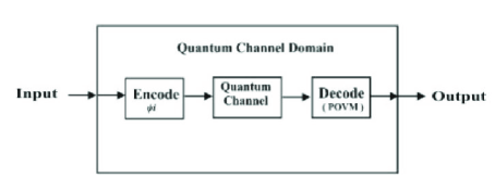
Figure 5-1: Communication through quantum channel

5.1 Quantum Data

Classical data is a string of classical bits. A classical bit consists of many quantum systems. It is represented by $0$ and $1$ known as Boolean states. A bit encoded in a system can take one of the two possible distinct values. For example, a bit on a compact disk means whether a laser beam is reflected or not reflected from its surface; on a credit card it is stored in the magnetization properties of a series of tiny domains; and for a computer a bit is the presence or the absence of voltage on tiny wires. A qubit, on the other hand is a microscopic system such as an atom or nuclear spin or a polarization of photon. A pair of quantum states that can reliably be distinguished are used to represent the Boolean states $0$ and $1\$[15]. Spin up and spin down of an electron and horizontal and vertical polarizations of a photon are among the remarkable examples. Furthermore a qubit can also exist in superposition states. In two dimensional Hilbert space spanned by unit vectors $\left|0\right\rangle$ and $\left|1\right\rangle$, a qubit can exist in state $\alpha\left|0\right\rangle+\beta\left|1\right\rangle$, $(\left|\alpha\right|^{2}+\left|\beta\right|^{2}=1)$. Physically it means that for any measurement that can discriminate between $\left|0\right\rangle$ and $\left|1\right\rangle$ the state $\alpha\left|0\right\rangle+\beta\left|1\right\rangle$ gives $\left|0\right\rangle$ with probability $\left|\alpha\right|^{2}$ and $\left|1\right\rangle$ with probability $\left|\beta\right|^{2}$. The state of two qubit system is a vector in the tensor product space spanned by basis $\left|00\right\rangle$, $\left|01\right\rangle$, $\left|10\right\rangle$, $\left|11\right\rangle.$ In tensor product space there exist entangled states which have no classical counterpart (see subsection 3.2.4 for detail).

A $n$ bit string of classical data can exist in any $2^{n}$ states from $x=00.......0$ to $11.....1.$ Similarly a string of $n$ qubits can exist in any state of the form

$$\left|\psi\right\rangle=\overset{11...1}{\underset{x=00...0}{\sum}}c_{x}\left|x\right\rangle,$$ (5.1)

where $c_{x}$ are the complex numbers such that $\underset{x}{\sum}\left|c_{x}\right|^{2}=1.$

5.2 von Neumann Entropy

If a quantum source is emitting quantum states $\left|\psi_{i}\right\rangle$ with probability $p_{i}$ then the minimum numbers of the qubits into which the source can be compressed by a quantum encoder such that it can reliably be decoded is given by von Neumann entropy of the source. von Neumann entropy is the quantum analogue of Shannon entropy and is mathematically defined as

$$S\left(\rho\right)=-\text{Tr}\left(\rho\log_{2}\rho\right),$$ (5.2)

where $\rho=\underset{i}{\sum}p_{i}\left|\psi_{i}\right\rangle\left\langle\psi_{i}\right|$. If $\lambda_{x}$ are the eigenvalues of $\rho$ then von Neumann entropy can be expressed as

$$S\left(\rho\right)=-\underset{x}{\sum}\lambda_{x}\log_{2}\lambda_{x},$$ (5.3)

where by definition $0\log_{2}0=0.$

5.3 The Holevo Bound

Holevo bound is the upper bound on the accessible information from a quantum system [91]. Let Alice prepares a quantum system $\rho_{x}$ where $x=0,1,....,n$ with probabilities $p_{1,}p_{2},....p_{n}$ and Bob performs the measurement on the system using POVM elements $\{E_{1},E_{2},...,E_{n}\}.$ Then the Holevo bound is given by

$$H\left(X:Y\right)\leq S\left(\rho\right)-\underset{x}{\sum}p_{x}S\left(\rho_{x}\right),$$ (5.4)

where $\rho=\underset{x}{\sum}p_{x}\rho_{x},$ and $H\left(X:Y\right)$ is mutual information of $X$ and $Y$ which measures how much information $X$ and $Y$ have in common [22].

5.4 Quantum Channels

A quantum channel is a completely positive trace preserving linear map from input state density matrices to output state density matrices [92, 93]. A positive map transforms the matrices with non-negative eigenvalues to the matrices with non-negative eigenvalues. On the other hand if the system of interest is a part of the larger system $A$ and $\varepsilon_{B}$ is a map such that $\varepsilon_{B}(\rho_{B})\rightarrow\rho_{B}^{\prime}$ then $\varepsilon_{B}$ is completely positive if and only if $\left(I_{A}\otimes\varepsilon_{B}\right)\left(\rho_{A}\otimes\rho_{B}\right)$ is also a positive map [92].

If $\rho$ and $\rho^{\prime}$are the input and output density matrices, respectively, then the channel dynamics in operator sum representation, is described as

$$\rho^{\prime}=\varepsilon(\rho)=\underset{k}{\sum}A_{k}^{\dagger}\rho A_{k},$$ (5.5)

where $\varepsilon$ is completely positive trace preserving linear map and $A_{k}$’s are the Kraus operators of a quantum channel. Let Alice wants to send a message to Bob using a quantum channel. She prepares a input signal state $\rho_{k}$ with probability $p_{k}.$ Then the corresponding ensemble of input states is given as $\rho=\underset{k}{\sum}p_{k}\rho_{k}$. On receiving the quantum states, Bob performs the measurement by using POVM to determine the state of the signal. According to the Holevo bound (Sec. 5.3) the mutual information accessible between Alice and Bob is

$$I\left(p_{k},\rho_{k}^{{\acute{}}}\right)=S(\underset{k}{\sum}p_{k}\rho_{k}^{{\acute{}}})-\underset{k}{\sum}p_{k}S(\rho_{k}^{{\acute{}}}),$$ (5.6)

where

$$S(\zeta)=-\text{Tr}\left(\zeta\log_{2}\zeta\right),$$ (5.7)

is von-Neumann entropy for the density matrix $\zeta.$ For the $n$ uses of a memoryless quantum channel with a given input entangled state the output becomes:

$$\rho^{{\acute{}}}=\Phi(\rho)=\underset{k_{1},....k_{n}}{\sum}(A_{k_{n}}\otimes...\otimes A_{k_{1}})^{\dagger}\rho_{e}(A_{k_{n}}\otimes...\otimes A_{k_{1}}),$$ (5.8)

where $\rho_{e}$ is some entangled state. According to the Eq. (5.6) the maximum amount of reliable information that can be transmitted along the channel is given as [89, 91],

$$C^{\left(n\right)}=\frac{1}{n}\sup_{p_{k},\rho_{k}^{\prime{\acute{}}}}I^{\left(n\right)}(p_{k},\rho_{k}^{{\acute{}}}),$$ (5.9)

here $n$ stands for the number of times the channel is used. The use of the entangled states as an input is interesting since there is a possibility of superadditivity of channel capacity, i.e., $I_{n+m}>I_{n}+I_{m}$. For the multiple uses of the channel the classical capacity $C$ of quantum channel is defined as

$$C=\underset{n\longrightarrow\infty}{\lim}C^{\left(n\right)}.$$ (5.10)

 The important examples of the quantum channels are depolarizing channel, phase damping channel and the amplitude damping channel. Next we explain these one by one.

5.4.1 Depolarizing Channel

Depolarizing channel models the decohering qubit that particularly has a nice symmetry. It can cause bit flip, phase flip or both. Under the action of this channel pure input state $\left|\psi\right\rangle$ is transformed into $\sigma_{x}\left|\psi\right\rangle$, $\sigma_{y}\left|\psi\right\rangle$, $\sigma_{z}\left|\psi\right\rangle$ with equal probability in addition to retaining its original form [47]. Here $\sigma_{x}$, $\sigma_{y}$, $\sigma_{z}$ are the Pauli matrices. The Kraus operators [22] for this channel are

$$A_{0} = \left(\sqrt{1-p}\right)I,$$

$$A_{1} = \sqrt{\frac{p}{3}}\sigma_{x},$$

$$A_{2} = \sqrt{\frac{p}{3}}\sigma_{y},$$

$$A_{3} = \sqrt{\frac{p}{3}}\sigma_{z}.$$ (5.11)

The state of a quantum system $\rho$ after this noise operation becomes

$$\acute{\rho}=\underset{k}{\sum}A_{k}\text{ }\rho\text{ }A_{k}^{\dagger}=\left(1-p\right)\rho+\frac{p}{3}\left(\sigma_{x}\rho\sigma_{x}+\sigma_{y}\rho\sigma_{y}+\sigma_{z}\rho\sigma_{z}\right).$$ (5.12)

Its effect on the Bloch sphere is given as

$$\left(r_{x},r_{y},r_{z}\right)\rightarrow\left(\left(1-\frac{4}{3}p\right)r_{x},\left(1-\frac{4}{3}p\right)r_{y},\left(1-\frac{4}{3}p\right)r_{z}\right).$$ (5.13)

Physically it means that under the action of depolarizing channel the Bloch sphere shrinks uniformly along the x,y,z by a shrinking factor $1-\frac{4}{3}p.$ The effect of depolarizing channel on a Bloch sphere is shown in figure 5-2 for $p=0.3.$

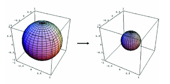
Figure 5-2: Evolution of Bloch sphere after passing through depolarizing channel with p=.3.

5.4.2 Phase Damping Channel

In phase damping channel information is lost without any loss of energy. This type of noise is unique to quantum mechanics. Kraus operators for this channel are

$$A_{0} = \sqrt{1-\frac{p}{2}}I,$$

$$A_{1} = \sqrt{\frac{p}{2}}\sigma_{z}.$$ (5.14)

Under the action of this channel the density matrix $\rho$ transforms as

$$\acute{\rho}=\left(1-\frac{p}{2}\right)\rho+\frac{p}{2}\sigma_{z}\rho\sigma_{z}.$$ (5.15)

Phase damping channel transforms the Bloch sphere as

$$\left(r_{x},r_{y},r_{z}\right)\rightarrow\left(\left(1-p\right)r_{x},\left(1-p\right)r_{y},r_{z}\right).$$ (5.16)

The above transformation means that the phase damping channel leaves the z-axis of the Bloch sphere unchanged whereas x-y plane is uniformly contracted by a factor of $\left(1-p\right).$ The effect of phase damping channel on Bloch sphere is shown in figure 5-3 for $p=0.2.$

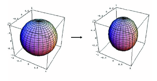
Figure 5-3: Evolution of Bloch sphere after passing through phase daming channel at p=.2.

5.4.3 Amplitude Damping Channel

This channel models the loss of energy from the quantum system. Kraus operators for this channel are [47]

$$A_{0} = \left[\begin{array}[]{cc}1&0\\ 0&\sqrt{1-p}\end{array}\right],$$ (5.19)

$$A_{1} = \left[\begin{array}[]{cc}0&\sqrt{p}\\ 0&0\end{array}\right].$$ (5.22)

The operator $A_{1}$ changes the state from $\left|1\right\rangle$ to $\left|0\right\rangle$ which is physically a process of losing energy to environment. The operator $A_{0}$ leaves $\left|0\right\rangle$ unchanged but reduces the amplitude of $\left|1\right\rangle.$ Amplitude damping channel transforms the Bloch sphere as

$$\left(r_{x},r_{y},r_{z}\right)\rightarrow\left(\left(\sqrt{1-p}\right)r_{x},\left(\sqrt{1-p}\right)r_{y},p+\left(1-p\right)r_{z}\right).$$ (5.23)

The effect of amplitude damping channel on Bloch sphere is shown in figure 5-4 for $p=0.5$.

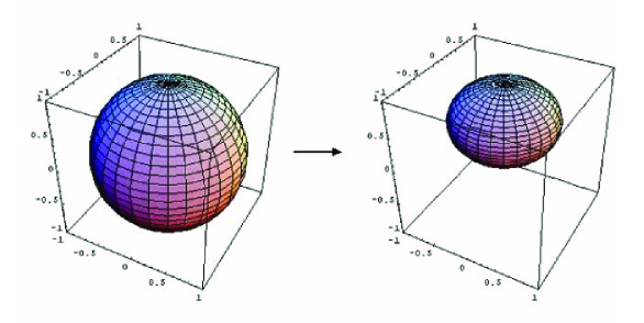
Figure 5-4: The effect of amplitude damping channel on Bloch sphere, for p=.5.

5.5 Channel Capacity

Channel capacity is the maximum reliable information that can be transmitted across the channel. Unlike classical channel, quantum channels can have various types of capacities. These include [25]

• Classical capacity C is the maximum asymptotic rate at which classical bits can be transmitted reliably across the quantum channel with the help of quantum encoder and decoder.

• Quantum capacity Q is the maximum asymptotic rate at which qubits are transmitted across the channel with quantum encoder and decoder

• The classically assisted quantum capacity $Q_{2\text{ }}$is the maximum asymptotic rate of reliable qubit transmission with the help of unlimited use of two way classical side channel between sender and receiver.

• The entanglement assisted channel capacity $C_{E}$ is the maximum asymptotic rate of reliable bit transmission with the help of unlimited prior entanglement between sender and receiver.

It is further to be noted that the classical channel capacity of a quantum channel can further be subdivided into four types [40] depending upon the input quantum states and the measurement basis. These four possible capacities are:

• $C_{PP}$ when the data is encoded in the form of product states at the sender end and the measurement at the receiver end is also of the product form.

• $C_{PE\text{ }}$ is the information capacity when the input data is encoded in the form of product states and the measurement at the receiver end is of the entangled form.

• $C_{EP}$ is the classical channel capacity for the input data is encoded in entangled states and the measurement at the receiver end is of the product form.

• $C_{EE}$ is the channel capacity for the case when both encoding and decoding is of entangled form.

5.6 No Cloning Theorem

One of the fundamental differences between classical information and quantum information is that classical information can perfectly be cloned or copied where as quantum information cannot be cloned. This is due to the reason that we cannot measure an unknown quantum state. Therefore if we are given two non-orthogonal quantum states $\left|\psi\right\rangle,\left|\phi\right\rangle$ and asked to distinguish them, there is no measurement which could distinguish them perfectly and we always have a probability of error. If it were possible to make many copies of the unknown states then we could repeat the optimal measurement to make the probability of error arbitrarily small. The no cloning theorem [24] states that this is not physically possible. Only the set of mutually orthogonal quantum states can be copied by a single unitary operator.

Let there be an unknown quantum state of the form

$$\left|\psi\right\rangle=a\left|0\right\rangle+b\left|1\right\rangle,$$ (5.24)

where $\left|a\right|^{2}+\left|b\right|^{2}=1$ and a unitary transformation $U_{cl}$ capable of cloning unknown states then

$$\left|\psi\right\rangle\left|0\right\rangle\overset{U_{cl}}{\rightarrow}\left|\psi\right\rangle\left|\psi\right\rangle=\left|a\right|^{2}\left|00\right\rangle+\left|b\right|^{2}\left|11\right\rangle+ab\left|01\right\rangle+ab\left|10\right\rangle.$$ (5.25)

On the other hand if we clone the expansion of $\left|\psi\right\rangle$ then we get

$$\left(a\left|0\right\rangle+b\left|1\right\rangle\right)\left|0\right\rangle\overset{U_{cl}}{\rightarrow}a\left|00\right\rangle+b\left|11\right\rangle.$$ (5.26)

Comparing the expressions (5.25) and (5.25) we see a clear contradiction. Hence quantum state cannot be copied.

5.7 Quantum Cryptography

Cryptography provides the techniques of making messages unintelligible to any undesired party. For this purpose the sender, Alice shares a secret key with receiver, Bob. In the course of time when Alice wants to send a secret message to Bob, she encrypts it using secret key. On receiving the encrypted message, Bob decrypts it with the help of the secret key. Any unauthorized party, Eve, being unaware of secret key cannot understand the message. There have been many protocols for classical cryptography from mere transposition and substitutions to modern sophisticated cryptosystems such as one time pads and RSA public cryptography [94, 95]. In one time pads, prior to any communication, the sender and legitimate receiver exchange secret keys through some physical mean and then store them at a safe and secure location. However the security of the keys can never be guaranteed, for Eve can copy the keys while being exchanged or from either party’s possession. In public key cryptosystems, such as, RSA, the receiver generates a pair of keys: a public key and a private key [96]. The security of the communication relies on determining the prime factors of a large integer. It is generally believed that the number of steps a classical computer would need to factorize an N decimal digit, grows exponentially with N. With recent advances in quantum computing, it is now possible to factorize very large numbers much faster [18]. As a result the security of RSA will be at risk. This problem can easily be fixed by quantum cryptography.

Security of a message in quantum cryptography relies on the laws of quantum physics instead of computational complexity. The laws important to mention are

1. A quantum system cannot be observed without being perturbed.

2. Position and momentum of a particle or the polarization of a photon in horizontal-vertical basis and diagonal basis cannot be measured simultaneously.

3. An unknown quantum state cannot be duplicated.

These unique properties of the quantum mechanical systems are used for protecting the classical information from being tampered in a multiparty setting where all the parties do not trust each other. The first known property used for this task was coding secret information on non orthogonal quantum states. The idea was floated by Stephen Wiesner by introducing the concept of quantum money [9]. He assumed that let a bank issue currency such that with each currency note there is a random quantum sequence of non-orthogonal states. Whenever anybody tries to duplicate the currency note he will have to perform an impossible task of cloning non-orthogonal quantum states. Although there is a problem in this scheme as the quantum states will have decoherence time shorter than the inflationary half life of most of the currencies, therefore, only the issuing bank can check the validity of the currency. Thus the counterfeiter can pass a fake note to layman [97], yet the idea proved very fruitful for quantum key distribution  In 1984 Charles Bennett and Gilles Brassard [98] presented a protocol for key distribution that was based on the Wiesner idea. Since then numerous quantum cryptographic protocols have been proposed and most of them have been implemented experimentally [13, 99, 100, 101, 102, 103, 104].

5.8 Quantum Superdense Coding

Quantum superdense coding, introduced by Bennett and Weisner [105], provides one of the best examples of the use of quantum mechanics in information processing tasks. The basic principle of superdense coding is that each member from the set of Bell states given by Eq. (3.18) can be transformed to other member of the set by manipulating only one qubit of a state.

Let Alice and Bob share an entangled state of the form

$$\left|\psi^{+}\right\rangle=\frac{1}{2}\left(\left|00\right\rangle+\left|11\right\rangle\right).$$ (5.27)

Alice can encode message by applying the unitary operators $I,\sigma_{x},i\sigma_{y}$ or $\sigma_{z}$ on her qubit. For example, if she wants to send $00$ then she applies the identity operator, $I,$ on her qubit so the original state $\left|\psi^{+}\right\rangle$ is retained; if she wants to send $01$ then she applies $\sigma_{z}$ to her qubit and the shared Bell state transforms to $\left|\psi^{-}\right\rangle;$ for sending $10$ she applies $\sigma_{x}$ on her qubit and the shared state becomes $\left|\phi^{+}\right\rangle$ and for $11$ she applies $i\sigma_{y}$ so that the shared state changes to $\left|\phi^{-}\right\rangle$, where $\left|\psi^{-}\right\rangle,\left|\phi^{+}\right\rangle$ and $\left|\phi^{-}\right\rangle$ are the members of Bell states set as defined in Eq. (3.18). The resulting four Bell states are orthogonal to each other and can easily be discriminated. In this way Alice can send two bits of classical information to Bob while interacting only with single qubit. Quantum superdense protocol is shown in figure 5-5.

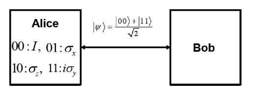
Figure 5-5: Quantum superdense coding

5.9 Teleportation

In quantum teleportation a sender, Alice teleports an unknown state $\left|\psi\right\rangle=\alpha\left|0_{A}\right\rangle+\beta\left|1_{A}\right\rangle$ $(\left|\alpha\right|^{2}+\left|\beta\right|^{2}=1)$ to a receiver Bob with whom she shares an EPR pair. Assume Alice and Bob share an entangled state $\left|\psi^{+}\right\rangle$. Alice interacts the qubit to be teleported with half of her EPR pair so the input state becomes

$$\left|\psi_{0}\right\rangle=\left|\psi\right\rangle\left|\psi^{+}\right\rangle=\frac{1}{\sqrt{2}}\left[\alpha\left|0_{A}\right\rangle\left(\left|0_{A}0_{B}\right\rangle+\left|1_{A}1_{B}\right\rangle\right)+\beta\left|1_{A}\right\rangle\left(\left|0_{A}0_{B}\right\rangle+\left|1_{A}1_{B}\right\rangle\right)\right],$$ (5.28)

where the subscripts $A$ and $B$ are for Alice and Bob respectively. Then she sends her qubits through a CNOT gate so that Eq. (5.28) becomes

$$\left|\psi_{1}\right\rangle=\frac{1}{2}\left[\alpha\left|0_{A}\right\rangle\left(\left|0_{A}0_{B}\right\rangle+\left|1_{A}1_{B}\right\rangle\right)+\beta\left|1_{A}\right\rangle\left(\left|1_{A}0_{B}\right\rangle+\left|0_{A}1_{B}\right\rangle\right)\right],$$ (5.29)

and then she sends her first qubit through Hadamard gate and Eq. (5.29) transforms to

$$\left|\psi_{2}\right\rangle=\frac{1}{2}\left[\alpha\left(\left|0_{A}\right\rangle+\left|1_{A}\right\rangle\right)\left(\left|0_{A}0_{B}\right\rangle+\left|1_{A}1_{B}\right\rangle\right)+\beta\left(\left|0_{A}\right\rangle-\left|1_{A}\right\rangle\right)\left(\left|1_{A}0_{B}\right\rangle+\left|0_{A}1_{B}\right\rangle\right)\right].$$ (5.30)

Rearranging Eq. (5.30) we get

$$\left|\psi_{2}\right\rangle = \frac{1}{2}\left[\left|0_{A}0_{A}\right\rangle\left(\alpha\left|0_{B}\right\rangle+\beta\left|1_{B}\right\rangle\right)+\left|0_{A}1_{A}\right\rangle\left(\left(\alpha\left|1_{B}\right\rangle+\beta\left|0_{B}\right\rangle\right)\right)\right.$$ (5.31)

$$+\left.\left|1_{A}0_{A}\right\rangle\left(\alpha\left|0_{B}\right\rangle-\beta\left|1_{B}\right\rangle\right)+\left|1_{A}1_{A}\right\rangle\left(\left(\alpha\left|1_{B}\right\rangle-\beta\left|0_{B}\right\rangle\right)\right)\right].$$

Now Alice performs measurement on the qubits in her possession. The measurement gives her one of the four possible classical bits, $\left|0_{A}0_{A}\right\rangle,\left|0_{A}1_{A}\right\rangle,\left|1_{A}0_{A}\right\rangle,\left|1_{A}1_{A}\right\rangle.$ If the outcome is $\left|0_{A}0_{A}\right\rangle$ then Bob’s state will be $\alpha\left|0_{B}\right\rangle+\beta\left|1_{B}\right\rangle$ and for all other possible results Bob’s states are given as follows

$$\left|0_{A}1_{A}\right\rangle\rightarrow\alpha\left|1_{B}\right\rangle+\beta\left|0_{B}\right\rangle,$$

$$\left|1_{A}0_{A}\right\rangle\rightarrow\alpha\left|0_{B}\right\rangle-\beta\left|1_{B}\right\rangle,$$

$$\left|1_{A}1_{A}\right\rangle\rightarrow\alpha\left|1_{B}\right\rangle-\beta\left|0_{B}\right\rangle.$$

Alice sends these results to Bob over a classical channel. When Bob comes to know these results then he fixes up his state to recover the original state $\left|\psi\right\rangle$ by applying the appropriate quantum gates. For example, if Bob receives $\left|0_{A}0_{A}\right\rangle$ he needs to do nothing i.e. he will apply the identity operator $I.$ If the outcome is $\left|0_{A}1_{A}\right\rangle$ then he will have to apply $X$ gate to fix up the state. Similarly if he obtains $\left|1_{A}0_{A}\right\rangle$ and $\left|1_{A}1_{A}\right\rangle$ then he can fix up the state by applying $Z$ gate and $XZ$ gate respectively. Quantum teleportation protocol is shown in the figure (5-6).

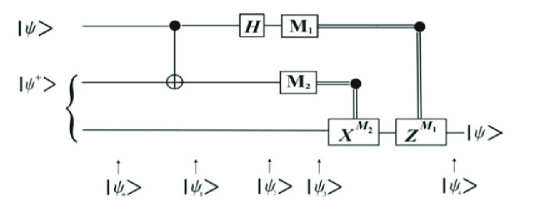
Figure 5-6: Quantum circuit for teleporting a qubit.

5.10 Quantum State Discrimination

The state of a classical system is described by its dynamical variables. For example the state of a one dimensional point particle can be given by its momentum $p$ and position $q$. There are no fundamental limitations on making these values more precise by refining the measurement process. This is because of the fact that the state variables are also the observables for a classical system. If the values of these variables along with the equations governing the dynamics of the system are exactly known then the future state of the system can be predicted correctly. The state of the quantum system is described by a normalized vector $\left|\psi\right\rangle$ in a complex linear vector space known as Hilbert space. These state vectors are not observables of quantum mechanics. Therefore, when one tries to read information stored in these state vectors after a desired processing of the states, he faces a lot of problem. When the information is encoded in known orthogonal states then decoding is relatively simple but if  the states are non orthogonal and even known, these cannot be discriminated perfectly. Discriminating among non orthogonal states is one of the burning issues of quantum information theory. For this purpose various strategies have been developed. Historically the first quantum state discrimination strategy, known as quantum hypothesis testing, was introduced by Helstorm [106]. It works on the principle of seeking the best guess on each trial while minimizing the rate of incorrect guesses. Hence one can always find an optimal strategy for discriminating between two non orthogonal quantum states using von Neumann projective measurement [106]. This strategy has was implemented experimentally by Barnett and Riis [107] using photon polarizing states as non-orthogonal quantum states. Another interesting strategy for discriminating among non-orthogonal quantum states, known as unambiguous state discrimination, was introduced by I. D. Ivanovic [108]. For the case of two non orthogonal quantum states Ivanovic studied the following problem. A preparator prepares a collection of quantum systems in a set of two known non-orthogonal quantum states and hands them over to an observer one by one for discrimination. He showed that if the observer is allowed to obtain inconclusive results occasionally then for the other cases he can perform error free discrimination between the given non-orthogonal states. Since then various strategies have been developed for optimal state discrimination [109, 110, 111, 112, 113].

5.11 Quantum State Tomography

All information about a quantum system is encoded in the state of a system but it is one of the great challenges for experimentalists to measure the state of the quantum system perfectly [114]. This is because of the fact that the state is not an observable in quantum mechanics [115] and therefore, it is not possible to perform all measurements on the single state to extract the whole information about the system. It is also impossible to create a perfect copy of an unknown quantum state [24]. Therefore, there is no way, even in principle, to infer the quantum state of a single system without some prior knowledge about it [116]. However it becomes possible to estimate the unknown quantum state of a system when many identical copies of the system are available. This procedure of reconstructing an unknown quantum state through a series of measurements on a number of identical copies of the system is called quantum state tomography. Each measurement gives a new dimension of system. To reconstruct the exact state of the system infinite number of copies are required. This type of procedure was first addressed by Fano [117] and remained mere speculation until original proposal for quantum tomography and its experimental verification [116, 118, 119]. Since than it has been applied successfully to the measurement of photon statistics of a semiconductor laser [120], reconstruction of density matrix of squeezed vacuum [121] and probing the entangled states of light and ions [122].

In the following we present a brief introduction to single qubit tomography following Refs. [22, 123].

5.11.1 The Stokes Parameters Representation of Qubit

Any single qubit density matrix $\rho$ can uniquely be represented with the help of three parameters $\left\{S_{1},S_{2},S_{3}\right\}$ and Pauli matrices $\sigma_{i}^{\prime}s$ by the expression

$$\rho=\frac{1}{2}\underset{i=0}{\overset{3}{\mathop{\textstyle\sum}}}S_{i}\sigma_{i},$$ (5.32)

where $S_{0}=1$ and the other parameters obey the relation $\underset{i=0}{\overset{3}{\mathop{\textstyle\sum}}}S_{i}^{2}\leq 1$. The parameters, $S_{i}$ are called Stokes parameters and for a quantum state $\rho$ these can be calculated as

$$S_{i}=\text{Tr}\left(\sigma_{i}\rho\right).$$ (5.33)

Physically these parameters give the outcome of a projective measurements as

$$S_{0} = P_{\left|0\right\rangle}+P_{\left|1\right\rangle}$$

$$S_{1} = P_{\frac{1}{\sqrt{2}}\left(\left|0\right\rangle+\left|1\right\rangle\right)}-P_{\frac{1}{\sqrt{2}}\left(\left|0\right\rangle-\left|1\right\rangle\right)}$$

$$S_{2} = P_{\frac{1}{\sqrt{2}}\left(\left|0\right\rangle+i\left|1\right\rangle\right)}-P_{\frac{1}{\sqrt{2}}\left(\left|0\right\rangle-i\left|1\right\rangle\right)}$$

$$S_{3} = P_{\left|0\right\rangle}-P_{\left|1\right\rangle}$$ (5.34)

where $P_{\left|i\right\rangle}$ is the probability to measure state $\left|i\right\rangle$ given by

$$P_{\left|i\right\rangle} = \left\langle i\right|\rho\left|i\right\rangle$$ (5.35)

$$= \text{Tr}\left(\left|i\right\rangle\left\langle i\right|\rho\right).$$

If we are provided with many copies of a quantum state then with the help of orthogonal set of matrices $\frac{\sigma_{0}}{\sqrt{2}},\frac{\sigma_{1}}{\sqrt{2}},\frac{\sigma_{2}}{\sqrt{2}},\frac{\sigma_{3}}{\sqrt{2}}$ the density matrix (5.32) can be written as

$$\rho=\frac{\text{{Tr}}(\rho)\sigma_{0}+\text{{Tr}}(\rho\sigma_{1})\sigma_{1}+\text{{Tr}}(\rho\sigma_{2})\sigma_{2}+\text{{Tr}}(\rho\sigma_{3})\sigma_{3}}{2}.$$ (5.36)

where the expression like Tr$(\rho\sigma_{i})$ represents the expectation value of the observable. For example to estimate Tr$(\rho\sigma_{3})$ we measure $\sigma_{3}$ for $m$ numbers of time giving the values $z_{1},z_{2,}.....,z_{m}$ all equal to +1 or -1. The average $\mathop{\textstyle\sum}\frac{z_{i}}{m_{i}}$ is an estimate to true value of the quantity Tr$(\rho\sigma_{3}).$ By central limit theorem this estimate has standard deviation $\frac{\Delta\sigma_{3}}{m}$ where $\Delta\sigma_{3}$ is the standard deviation for single measurement of $\sigma_{3}$ that is upper bounded by 1. Therefore, the standard deviation for estimate $\mathop{\textstyle\sum}\frac{z_{i}}{m_{i}}$ is at most $\frac{i}{\sqrt{m}}.$The standard deviation for each of the measurement in Eq. (5.36) is the same [22]. In this way with the help of Eq. (5.36) tomography can be performed for an unknown single qubit state.

5.11.2 Single Qubit Tomography

A single qubit state can very conveniently be represented by a vector in three dimensional vector space spanned by Pauli matrices. This representation provides very helpful way for geometrical visualization of single qubit state, where all the legal states fall within a unit sphere (Bloch sphere). In this representation all the pure states lie on the surface of the sphere and mixed states fall inside the sphere. The pure states can be written as

$$\left|\psi\right\rangle=\cos\frac{\theta}{2}\left|0\right\rangle+e^{i\phi}\sin\frac{\theta}{2}\left|1\right\rangle$$ (5.37)

where $\theta$ and $\phi$ map them on the surface of the sphere. Any state $\left|\psi\right\rangle$ and its orthogonal component $\left|\psi^{\perp}\right\rangle$ fall on two opposite points on the surface of the sphere such that the line connecting these points form the axis of the sphere.

For the tomography of an unknown single qubit state three consecutive measurements are required. Each measurement gives one dimension of the system until one becomes aware of all dimensions after the complete set of measurement. For example, a single qubit state $\rho=\left|\psi\right\rangle\left\langle\psi\right|$ where $\left|\psi\right\rangle$ is defined in Eq. (5.37), can be expressed as

$$\rho=\frac{1}{2}\left(\sigma_{0}+\sin\theta\cos\phi\text{ }\sigma_{1}+\sin\theta\sin\phi\text{ }\sigma_{2}+\cos\theta\text{ }\sigma_{3}\right)$$ (5.38)

Comparing Eqs. (5.32) and (5.38) the Stokes parameters for this state become

$$S_{1}=\sin\theta\cos\phi,\text{ }S_{2}=\sin\theta\sin\phi,\text{ }S_{3}=\cos\theta.$$ (5.39)

For an unknown state of the form Eq. (5.38) when a measurement is performed in $\sigma_{3}$ basis it confines the state to a plane $z=\cos\theta$; as shown in Fig. (5-7).

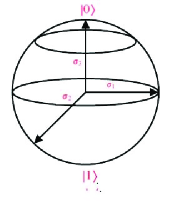
Figure 5-7: The measuremsnt in $\sigma_{3}$ basis confines the unkown quantum state to a plane $z=\cos\theta.$

Then a measurement in $\sigma_{2}$ basis is performed that further confines it to the plane $y=\sin\theta\sin\phi$. The combined effect of both these measurements restricts the unknown quantum state to a line parallel to x-axis as shown in Fig. (5-8).

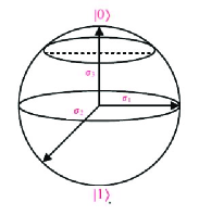
Figure 5-8: The measurement in $\sigma_{2}$ basis confines the state to $y=\sin\theta\sin\phi$ plane. When this measurement is combined with first measurement the unknown state reduces to a line parrallel to x-axis.

At last the measurement in $\sigma_{1}$ basis pinpoints the state as point lying on this line (resulting from the intersection of $y$ and $z$ planes) at distance $x=\sin\theta\cos\phi$; as illustrated in Fig. (5-9).

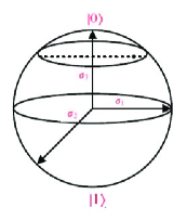
Figure 5-9: The last measurement in $\sigma_{1}$ basis pinpoints the state as point  that results from the intersection of three orthogonal planes.

Since the resultant state is due the intersection of three orthogonal planes therefore the order these measurements is immaterial in the whole process. In experimental analysis one usually faces three types of most prominent errors.

1. Errors due to measurement basis:- This type of errors appear by an accidental use of different measurement basis. It can be reduced by increasing the accuracy of the apparatus.

2. Errors due to counting statistics:- To extract full information about an unknown quantum state it requires infinite number of measurements. On the other hand all real life measurements can be performed on limited size of ensembles which is a source for this type of errors. This can be overcome by performing measurement on a larger ensemble.

3. Errors from experimental stability:- The drift can occur either in the state produces or due the efficiency of the detection system that can constrain the data collection time.

Chapter 6 Generalized Quantization Scheme for Two-Person Non-zero-Sum Games

There have been two well known quantization schemes for two person non-zero sum games. The first was presented by Eisert et al. [27] and the second by Marinatto and Weber [28]. The main purpose of this endeavour was to find a way for resolving dilemmas in games like Prisoners’ Dilemma and Battle of Sexes. These quantization schemes gave very interesting results when applied to different games [29, 30, 31, 32, 33, 34]. A detailed description of these schemes has been provided in section (4.2) and section (4.3) respectively.

In this chapter we introduce the generalized quantization scheme for two person non-zero sum games that gives a relationship between these two apparently different quantization schemes. The game of Battle of Sexes has been used as an example to introduce this quantization scheme but this scheme is applicable to other games as well. Separate set of parameters are identified for which this scheme reduces to that of Marinatto and Weber and Eisert et al. quantization schemes. Furthermore some other interesting situations are identified which are not apparent within the existing two quantizations schemes.

6.1 Comparison of Quantization Schemes

A straight forward comparison of Eisert et al. [27] and Marinatto and Weber [28] quantization schemes can be performed by making use of entanglement operator $\hat{J}$. It was pointed out by Eisert et al. [27] that the initial entangled state for quantum games can be prepared with the application of an entanglement operator $\hat{J}$ as

$$\left|\psi_{in}\right\rangle=\hat{J}(\frac{\gamma}{2})\left|CC\right\rangle,$$ (6.1)

where $\hat{J}$ is defined as

$$\hat{J}(\frac{\gamma}{2})=\exp(-i\frac{\gamma}{2}D\otimes D).$$ (6.2)

The qubits are forwarded one to the each player. The strategic moves of Alice and Bob are associated with the unitary operators $U_{1}(\theta_{1},\phi_{1})$ and $U_{2}(\theta_{2},\phi_{2})$, respectively. After the application of players moves the state of game is

$$\left|\psi_{f}\right\rangle=\left(U_{1}\otimes U_{2}\right)\hat{J}(\frac{\gamma}{2})\left|CC\right\rangle.$$ (6.3)

Then Alice and Bob return back their qubits to arbiter for measurement, the final state of the game prior to the measurement is

$$\left|\psi_{f}\right\rangle=\hat{J}^{\dagger}(\frac{\delta}{2})\left(U_{1}\otimes U_{2}\right)\hat{J}(\frac{\gamma}{2})\left|CC\right\rangle,$$ (6.4)

where

$$\hat{J}(\frac{\delta}{2})=\exp(-i\frac{\delta}{2}D\otimes D),$$ (6.5)

is the disentanglement operator. Putting$\ \delta=\gamma$ in (6.4) the original scheme of Eisert et al. [27] is reproduced and letting $\delta=0$ with restriction of $\hat{U}_{1}$ and $\hat{U}_{2}$ as a linear combination of identity operator $\hat{I},$ and the flip operator $\hat{C}$, the scheme of Marinatto and Weber [28] is retrieved.

6.2 Generalized Quantization Scheme

To introduce the generalized quantization scheme we take Battle of Sexes as an example which is an interesting static game of complete information with payoff matrix (2.6). For the quantization of this game we suppose that Alice and Bob are given the following initial state

$$\left|\psi_{in}\right\rangle=\cos\frac{\gamma}{2}\left|00\right\rangle+i\sin\frac{\gamma}{2}\left|11\right\rangle.$$ (6.6)

Here $\left|0\right\rangle$ and $\left|1\right\rangle$ represent the vectors in the strategy space corresponding to Opera and TV, respectively with $\gamma\in\left[0,\frac{\pi}{2}\right]$. Here $\gamma$ is entanglement of initial quantum state. The strategy of each of the players is represented by the unitary operator $U_{i}$ of the form 

$$U_{i}=\cos\frac{\theta_{i}}{2}R_{i}+\sin\frac{\theta_{i}}{2}C_{i},\text{ \ \ \ }$$ (6.7)

where $i=1$ or $2$ and $R_{i}$, $C_{i}$ are the unitary operators defined as

$$R_{i}\left|0\right\rangle =e^{i\phi_{i}}\left|0\right\rangle,\text{ \ \ }R_{i}\left|1\right\rangle=e^{-i\phi_{i}}\left|1\right\rangle,$$

$$C_{i}\left|0\right\rangle =-\left|1\right\rangle,\text{ \ \ \ \ \ }C_{i}\left|1\right\rangle=\left|0\right\rangle.$$ (6.8)

Here we restrict our treatment to two parameter set of strategies for mathematical simplicity in accordance with Ref. [27]. After the application of the strategies, the initial state given by Eq. (6.6) transforms into

$$\left|\psi_{f}\right\rangle=(U_{1}\otimes U_{2})\left|\psi_{in}\right\rangle.$$ (6.9)

Using Eqs. (6.8) and (6.9) the above expression becomes

$$\left|\psi_{f}\right\rangle =\cos\frac{\gamma}{2}[\cos\frac{\theta_{1}}{2}\cos\frac{\theta_{2}}{2}e^{i(\phi_{1}+\phi_{2})}\left|00\right\rangle-\cos\frac{\theta_{1}}{2}\sin\frac{\theta_{2}}{2}e^{i\phi_{1}}\left|01\right\rangle$$

$$-\cos\frac{\theta_{2}}{2}\sin\frac{\theta_{1}}{2}e^{i\phi_{2}}\left|10\right\rangle+\sin\frac{\theta_{1}}{2}\sin\frac{\theta_{2}}{2}\left|11\right\rangle]$$

$$+i\sin\frac{\gamma}{2}[\cos\frac{\theta_{1}}{2}\cos\frac{\theta_{2}}{2}e^{-i(\phi_{1}+\phi_{2})}\left|11\right\rangle+\cos\frac{\theta_{1}}{2}\sin\frac{\theta_{2}}{2}e^{-i\phi_{1}}\left|10\right\rangle$$

$$+\cos\frac{\theta_{2}}{2}\sin\frac{\theta_{1}}{2}e^{-i\phi_{2}}\left|01\right\rangle+\sin\frac{\theta_{1}}{2}\sin\frac{\theta_{2}}{2}\left|00\right\rangle].$$ (6.10)

The payoff operators for Alice and Bob corresponding to payoff matrix (2.6) are

$$P_{A} =\alpha P_{00}+\beta P_{11}+\sigma(P_{01}+P_{10}),$$

$$P_{B} =\alpha P_{11}+\beta P_{00}+\sigma(P_{01}+P_{10}),$$ (6.11)

where

$$P_{00} =\left|\psi_{00}\right\rangle\left\langle\psi_{00}\right|\text{, \ }\left|\psi_{00}\right\rangle=\cos\frac{\delta}{2}\left|00\right\rangle+i\sin\frac{\delta}{2}\left|11\right\rangle,$$ (6.12a)

$$P_{11} =\left|\psi_{11}\right\rangle\left\langle\psi_{11}\right|,\text{ \ }\left|\psi_{11}\right\rangle=\cos\frac{\delta}{2}\left|11\right\rangle+i\sin\frac{\delta}{2}\left|00\right\rangle,$$ (6.12b)

$$P_{10} =\left|\psi_{10}\right\rangle\left\langle\psi_{10}\right|\text{, \ }\left|\psi_{10}\right\rangle=\cos\frac{\delta}{2}\left|10\right\rangle-i\sin\frac{\delta}{2}\left|01\right\rangle,$$ (6.12c)

$$P_{01} =\left|\psi_{01}\right\rangle\left\langle\psi_{01}\right|\text{, \ }\left|\psi_{01}\right\rangle=\cos\frac{\delta}{2}\left|01\right\rangle-i\sin\frac{\delta}{2}\left|10\right\rangle,$$ (6.12d)

and $$\delta\in\left[0,\frac{\pi}{2}\right] \delta \gamma, \delta=0$$ refers to the entanglement of the measurement basis. Above payoff operators reduce to that of Eisert’s scheme for equal to which represents the entanglement of the initial state. For above operators transform into that of Marinatto and Weber’s scheme. In generalized quantization scheme payoffs for the players are calculated as

$$\$_{A}(\theta_{1},\phi_{1},\theta_{2},\phi_{2}) = \text{Tr}(P_{A}\rho_{f})\text{,}$$

$$\$_{B}(\theta_{1},\phi_{1},\theta_{2},\phi_{2}) = \text{Tr}(P_{B}\rho_{f}),$$ (6.13)

where $\rho_{f}=\left|\psi_{f}\right\rangle\left\langle\psi_{f}\right|$ is the density matrix for the quantum state given by Eq. (6.10) and Tr represents the trace of a matrix. Using Eqs. (6.10), (6.11) and (6.13) the payoffs for players are obtained as

$$\$_{A}(\theta_{1},\phi_{1},\theta_{2},\phi_{2}) =\cos^{2}\frac{\theta_{1}}{2}\cos^{2}\frac{\theta_{2}}{2}\left[\eta\sin^{2}\frac{\gamma}{2}+\xi\cos^{2}\frac{\gamma}{2}+\chi\cos 2(\phi_{1}+\phi_{2})\sin\gamma\right.$$

$$\left.-\sigma\right]+\sin^{2}\frac{\theta_{1}}{2}\sin^{2}\frac{\theta_{2}}{2}(\eta\cos^{2}\frac{\gamma}{2}+\xi\sin^{2}\frac{\gamma}{2}-\chi\sin\gamma-\sigma)$$

$$+\frac{(\alpha+\beta-2\sigma)\sin\gamma-2\chi}{4}\sin\theta_{1}\sin\theta_{2}\sin(\phi_{1}+\phi_{2})+\sigma,$$

(6.14a)

$$\$_{B}(\theta_{1},\phi_{1},\theta_{2},\phi_{2}) =\cos^{2}\frac{\theta_{1}}{2}\cos^{2}\frac{\theta_{2}}{2}\left[\xi\sin^{2}\frac{\gamma}{2}+\eta\cos^{2}\frac{\gamma}{2}-\chi\cos 2(\phi_{1}+\phi_{2})\sin\gamma\right.$$

$$\left.-\sigma\right]+\sin^{2}\frac{\theta_{1}}{2}\sin^{2}\frac{\theta_{2}}{2}(\xi\cos^{2}\frac{\gamma}{2}+\eta\sin^{2}\frac{\gamma}{2}+\chi\sin\gamma-\sigma)+$$

$$\frac{(\alpha+\beta-2\sigma)\sin\gamma+2\chi}{4}\sin\theta_{1}\sin\theta_{2}\sin(\phi_{1}+\phi_{2})+\sigma,$$

(6.14b)

where

$$\xi=\alpha\cos^{2}\frac{\delta}{2}+\beta\sin^{2}\frac{\delta}{2},$$ (6.15)

$$\eta=\alpha\sin^{2}\frac{\delta}{2}+\beta\cos^{2}\frac{\delta}{2},$$ (6.16)

$$\chi=\frac{(\alpha-\beta)}{2}\sin\delta.$$ (6.17)

Classical results can easily be found from Eqs. (6.14a) and (6.14b) by simply unentangling, the initial quantum state of the game i.e. letting $\gamma=0$. Furthermore all the results found by Marinatto and Weber [28] and Eisert et al. [27] are also embedded in these payoffs.

6.2.1 Reduction to Marinatto and Weber Quantization Scheme

The generalized quantization scheme reduces to Marinatto and Weber [28] quantization scheme for $\delta=0.$ In this situation we have following two cases of interest.

Case(a): When $\delta=0$ and $\phi_{1}=0$, $\phi_{2}=0.$ then the payoffs for the players from Eqs. (6.14a) and (6.14b) reduce to

$$\$_{A}(\theta_{1},\phi_{1,}\theta_{2},\phi_{2}) =\cos^{2}\frac{\theta_{1}}{2}[\cos^{2}\frac{\theta_{2}}{2}(\alpha+\beta-2\sigma)-\alpha\sin^{2}\frac{\gamma}{2}-\beta\cos^{2}\frac{\gamma}{2}+\sigma]$$

$$+\cos^{2}\frac{\theta_{2}}{2}(-\alpha\sin^{2}\frac{\gamma}{2}-\beta\cos^{2}\frac{\gamma}{2}+\sigma)+\alpha\sin^{2}\frac{\gamma}{2}+\beta\cos^{2}\frac{\gamma}{2},$$ (6.18a)

$$\$_{B}(\theta_{1},\phi_{1},\theta_{2},\phi_{2}) =\cos^{2}\frac{\theta_{2}}{2}[\cos^{2}\frac{\theta_{1}}{2}(\alpha+\beta-2\sigma)-\beta\sin^{2}\frac{\gamma}{2}-\alpha\cos^{2}\frac{\gamma}{2}+\sigma]$$

$$+\cos^{2}\frac{\theta_{1}}{2}(-\beta\sin^{2}\frac{\gamma}{2}-\alpha\cos^{2}\frac{\gamma}{2}+\sigma)+\beta\sin^{2}\frac{\gamma}{2}+\alpha\cos^{2}\frac{\gamma}{2}.$$ (6.18b)

These payoffs are the same as found by Marinatto and Weber [28] where the players apply the identity operators $$I_{1} I_{2} \cos^{2}\frac{\theta_{1}}{2} \cos^{2}\frac{\theta_{2}}{2}$$ and with probabilities and respectively on the given initial quantum state of the form of Eq. (6.6).

Case(b): When $\delta=0$ and $\phi_{1}+\phi_{2}=\frac{\pi}{2}$ then Eqs. (6.14a) and (6.14b) reduce to

$$\$_{A}(\theta_{1},\phi_{1},\theta_{2},\phi_{2}) =\cos^{2}\frac{\theta_{1}}{2}\left[\cos^{2}\frac{\theta_{2}}{2}(\alpha+\beta-2\sigma)-\alpha\sin^{2}\frac{\gamma}{2}-\beta\cos^{2}\frac{\gamma}{2}+\sigma\right]$$

$$+\cos^{2}\frac{\theta_{2}}{2}\left(-\alpha\sin^{2}\frac{\gamma}{2}-\beta\cos^{2}\frac{\gamma}{2}+\sigma\right)+\alpha\sin^{2}\frac{\gamma}{2}+\beta\cos^{2}\frac{\gamma}{2}$$

$$+\frac{\left(\alpha+\beta-2\sigma\right)}{4}\sin\gamma\sin\theta_{1}\sin\theta_{2},$$ (6.19a)

$$\$_{B}(\theta_{1},\phi_{1},\theta_{2},\phi_{2}) =\cos^{2}\frac{\theta_{2}}{2}\left[\cos^{2}\frac{\theta_{1}}{2}(\alpha+\beta-2\sigma)-\beta\sin^{2}\frac{\gamma}{2}-\alpha\cos^{2}\frac{\gamma}{2}+\sigma\right]$$

$$+\cos^{2}\frac{\theta_{1}}{2}\left(-\beta\sin^{2}\frac{\gamma}{2}-\alpha\cos^{2}\frac{\gamma}{2}+\sigma\right)+\beta\sin^{2}\frac{\gamma}{2}+\alpha\cos^{2}\frac{\gamma}{2}$$

$$+\frac{\left(\alpha+\beta-2\sigma\right)}{4}\sin\gamma\sin\theta_{1}\sin\theta_{2}.$$ (6.19b)

In the context of Marinatto and Weber scheme [28, 85] the above payoffs for the two players correspond to a situation when the strategies of the players are linear combination of operators $$I \hat{C} \hat{O}_{i}=\sqrt{p_{i}}\hat{I}+\sqrt{1-p_{i}}\hat{C} p_{i}=\cos^{2}\frac{\theta_{i}}{2} i=1 2$$ and flip operator of the form with probabilities , or and initial entangled state of the form given by Eq. (6.6).

6.2.2 Reduction to Eisert Quantization Scheme

The results of Eisert et al. [27] quantization scheme can be retrieved restricting $\delta=\gamma$ in the generalized quantization scheme. Here again we have two cases of interest.

Case (a) When $\delta=\gamma$ and$\ \phi_{1}\neq 0$, $\phi_{2}\neq 0$ then payoffs given by the Eqs. (6.14a) and (6.14b) very interestingly change to the payoffs as if the game has been quantized using Eisert et al. [27] scheme for the initial quantum state of the form (6.6). In this situation the payoffs for both the players are

$$\$_{A}(\theta_{1},\phi_{1},\theta_{2},\phi_{2}) =\cos^{2}\frac{\theta_{1}}{2}\cos^{2}\frac{\theta_{2}}{2}\left[\eta_{1}\sin^{2}\frac{\gamma}{2}+\xi_{1}\cos^{2}\frac{\gamma}{2}+\chi_{1}\cos 2(\phi_{1}+\phi_{2})\right.$$

$$\left.-\sigma\right]+\sin^{2}\frac{\theta_{1}}{2}\sin^{2}\frac{\theta_{2}}{2}\left(\eta_{1}\cos^{2}\frac{\gamma}{2}+\xi_{1}\sin^{2}\frac{\gamma}{2}-\chi_{1}-\sigma\right)$$

$$+\frac{\left(\beta-\sigma\right)}{2}\sin\gamma\sin\theta_{1}\sin\theta_{2}\sin\left(\phi_{1}+\phi_{2}\right)+\sigma,$$ (6.20a)

$$\$_{B}(\theta_{1},\phi_{1},\theta_{2},\phi_{2}) =\cos^{2}\frac{\theta_{1}}{2}\cos^{2}\frac{\theta_{2}}{2}\left[\xi_{1}\sin^{2}\frac{\gamma}{2}+\eta_{1}\cos^{2}\frac{\gamma}{2}-\chi_{1}\cos 2\left(\phi_{1}+\phi_{2}\right)\right.$$

$$\left.-\sigma\right]+\sin^{2}\frac{\theta_{1}}{2}\sin^{2}\frac{\theta_{2}}{2}\left(\xi_{1}\cos^{2}\frac{\gamma}{2}+\eta_{1}\sin^{2}\frac{\gamma}{2}+\chi_{1}-\sigma\right)$$

$$+\frac{\left(\alpha-\sigma\right)}{2}\sin\gamma\sin\theta_{1}\sin\theta_{2}\sin\left(\phi_{1}+\phi_{2}\right)+\sigma,$$ (6.20b)

where

$$\xi_{1}=\alpha\cos^{2}\frac{\gamma}{2}+\beta\sin^{2}\frac{\gamma}{2},$$

$$\eta_{1}=\alpha\sin^{2}\frac{\gamma}{2}+\beta\cos^{2}\frac{\gamma}{2},$$

$$\chi_{1}=\frac{(\alpha-\beta)}{2}\sin^{2}\gamma.$$

To draw a better comparison we take $\delta=\gamma=\frac{\pi}{2}$ then the payoffs given by Eqs. (6.20) reduce to

$$\$_{A}(\theta_{1},\phi_{1},\theta_{2},\phi_{2}) =\left(\alpha-\sigma\right)\cos^{2}\frac{\theta_{1}}{2}\cos^{2}\frac{\theta_{2}}{2}\sin^{2}\left(\phi_{1}+\phi_{2}\right)$$

$$+\left(\beta-\sigma\right)\left[\cos\frac{\theta_{1}}{2}\cos\frac{\theta_{2}}{2}\sin(\phi_{1}+\phi_{2})+\sin\frac{\theta_{1}}{2}\sin\frac{\theta_{2}}{2}\right]^{2}+\sigma,$$ (6.21a)

$$\$_{B}(\theta_{1},\phi_{1},\theta_{2},\phi_{2}) =\left(\alpha-\sigma\right)\left[\cos\frac{\theta_{1}}{2}\cos\frac{\theta_{2}}{2}\sin(\phi_{1}+\phi_{2})+\sin\frac{\theta_{1}}{2}\sin\frac{\theta_{2}}{2}\right]^{2}$$

$$+\left(\beta-\sigma\right)\cos^{2}\frac{\theta_{1}}{2}\cos^{2}\frac{\theta_{2}}{2}\sin^{2}\left(\phi_{1}+\phi_{2}\right)+\sigma.$$ (6.21b)

The payoffs given in the Eqs. (6.21) have already been found by Du et al. [139] through Eisert et al. scheme [27].

Case (b) When $\delta=\gamma$ and$\ \phi_{1}=\phi_{2}=0$, then as shown by Eisert et al. [27, 72], one gets classical payoffs with mixed strategies. For a better comparison putting $\gamma=\delta=\frac{\pi}{2}$ and $\phi_{1}=\phi_{2}=0$ in the Eqs. (6.20a) and (6.20b) the same situation occurs and the payoffs reduce to

$$\$_{A}(\theta_{1},\phi_{1},\theta_{2},\phi_{2}) = \alpha\cos^{2}\frac{\theta_{1}}{2}\cos^{2}\frac{\theta_{2}}{2}+\beta\sin^{2}\frac{\theta_{1}}{2}\sin^{2}\frac{\theta_{2}}{2}$$ (6.22a)

$$+\sigma(\cos^{2}\frac{\theta_{1}}{2}\sin^{2}\frac{\theta_{2}}{2}+\sin^{2}\frac{\theta_{1}}{2}\cos^{2}\frac{\theta_{2}}{2}),$$

$$\$_{B}(\theta_{1},\phi_{1},\theta_{2},\phi_{2}) = \beta\cos^{2}\frac{\theta_{1}}{2}\cos^{2}\frac{\theta_{2}}{2}+\alpha\sin^{2}\frac{\theta_{1}}{2}\sin^{2}\frac{\theta_{2}}{2}$$ (6.22b)

$$+\sigma(\cos^{2}\frac{\theta_{1}}{2}\sin^{2}\frac{\theta_{2}}{2}+\sin^{2}\frac{\theta_{1}}{2}\cos^{2}\frac{\theta_{2}}{2}).$$

In this case the game behaves just like classical game where the players are playing mixed strategies with probabilities $$\cos^{2}\frac{\theta_{1}}{2} \cos^{2}\frac{\theta_{2}}{2}$$ and respectively.

6.2.3 New Explorations

These are the situations which do not arise in the original versions of Eisert et al. scheme [27] and Marinatto and Weber scheme [28].

Case (a): When $\delta\neq\gamma$ and $\phi_{1}=0$, $\phi_{2}=0$ the payoffs given by the Eqs. (6.14a) and (6.14b) reduce to

$$\$_{A}(\theta_{1},\phi_{1,}\theta_{2},\phi_{2} =\cos^{2}\frac{\theta_{1}}{2}\left[\cos^{2}\frac{\theta_{2}}{2}\left(\alpha+\beta-2\sigma\right)-\alpha\sin^{2}\frac{\left(\gamma-\delta\right)}{2}\right.$$

$$\left.-\beta\cos^{2}\frac{(\gamma-\delta)}{2}+\sigma\right]+\cos^{2}\frac{\theta_{2}}{2}\left[-\alpha\sin^{2}\frac{\left(\gamma-\delta\right)}{2}\right.$$

$$\left.-\beta\cos^{2}\frac{\left(\gamma-\delta\right)}{2}+\sigma\right]+\alpha\sin^{2}\frac{\left(\gamma-\delta\right)}{2}+\beta\cos^{2}\frac{\left(\gamma-\delta\right)}{2},$$ (6.23a)

$$\$_{B}\left(\theta_{1},\phi_{1,}\theta_{2},\phi_{2}\right) =\cos^{2}\frac{\theta_{2}}{2}\left[\cos^{2}\frac{\theta_{1}}{2}\left(\alpha+\beta-2\sigma\right)-\beta\sin^{2}\frac{\left(\gamma-\delta\right)}{2}\right.$$

$$\left.-\alpha\cos^{2}\frac{\left(\gamma-\delta\right)}{2}+\sigma\right]+\cos^{2}\frac{\theta_{1}}{2}\left[-\beta\sin^{2}\frac{\left(\gamma-\delta\right)}{2}\right.$$

$$\left.-\alpha\cos^{2}\frac{\left(\gamma-\delta\right)}{2}+\sigma\right]+\beta\sin^{2}\frac{\left(\gamma-\delta\right)}{2}+\alpha\cos^{2}\frac{\left(\gamma-\delta\right)}{2}.$$ (6.23b)

These payoffs are equivalent to Marinatto and Weber [28] when $\gamma$ is replaced with $\gamma-\delta.$

Case (b): When $\delta\neq 0$ and $\gamma=0$ then from Eqs. (6.20a) and (6.20b) the payoffs of the players reduce to

$$\$_{A}(\theta_{1},\phi_{1},\phi_{2},\theta_{2}) =\cos^{2}\frac{\theta_{1}}{2}\left[\cos^{2}\frac{\theta_{2}}{2}\left(\alpha+\beta-2\sigma\right)-\alpha\sin^{2}\frac{\delta}{2}-\beta\cos^{2}\frac{\delta}{2}+\sigma\right]$$

$$+\cos^{2}\frac{\theta_{2}}{2}\left(-\alpha\sin^{2}\frac{\delta}{2}-\beta\cos^{2}\frac{\delta}{2}+\sigma\right)+\alpha\sin^{2}\frac{\delta}{2}+\beta\cos^{2}\frac{\delta}{2}$$

$$-\frac{\left(\alpha-\beta\right)}{2}\sin\delta\sin\theta_{1}\sin\theta_{2}\sin\left(\phi_{1}+\phi_{2}\right),$$ (6.24a)

$$\$_{B}(\theta_{1},\phi_{1},\phi_{2},\theta_{2}) =\cos^{2}\frac{\theta_{2}}{2}\left[\cos^{2}\frac{\theta_{1}}{2}\left(\alpha+\beta-2\sigma\right)-\beta\sin^{2}\frac{\delta}{2}-\alpha\cos^{2}\frac{\delta}{2}+\sigma\right]$$

$$+\cos^{2}\frac{\theta_{1}}{2}\left(-\beta\sin^{2}\frac{\delta}{2}-\alpha\cos^{2}\frac{\delta}{2}+\sigma\right)+\beta\sin^{2}\frac{\delta}{2}+\alpha\cos^{2}\frac{\delta}{2}$$

$$+\frac{\left(\alpha-\beta\right)}{2}\sin\delta\sin\theta_{1}\sin\theta_{2}\sin\left(\phi_{1}+\phi_{2}\right).$$ (6.24b)

This shows that the measurement plays a crucial role in quantum games as if initial state is unentangled, i.e., $$\gamma=0, \delta \gamma.$$ arbiter can still apply entangled basis for the measurement to obtain quantum mechanical results. Above payoff’s are similar to that of Marinatto and Weber for the Battle of Sexes games if is replaced by

This encourages us to investigate the role of measurement in quantum games in more detail.

6.3 The Role of Measurement in Quantum Games

In two players quantum game arbiter prepares a two qubit initial quantum state and passes on one qubit to each of the players (generally referred to as Alice and Bob). After applying their local operators (or strategies) the players return the respective qubits back to arbiter who announces the payoffs after performing measurement by applying the suitable payoff operators depending on the payoff matrix of the game. The role of the initial quantum state remained an interesting issue in quantum games [27, 28, 30] see also section (4.4). However, the importance of the payoff operators, used by arbiter to perform measurement to determine the payoffs of the players, remained unnoticed. In chapter (6) we pointed out the importance of measurement basis in quantum games. It was shown that if the arbiter is allowed to perform the measurement in the entangled basis some interesting situations could arise which were not possible in the frame work of Eisert et al. [27] and Marinatto and Weber [28] schemes. Here we further extend this notion to investigate the role of measurement basis in quantum games by taking Prisoners’ Dilemma as an example. It is observed that the quantum payoffs can be divided into four different categories on the basis of initial state and measurement basis. These different situations arise due the possibility of having product or entangled initial state and then applying product or entangled basis for the measurement [124, 125]. In the context of our generalized framework for quantum games, the four different types of payoffs are 

(i) $\$_{PP}$ is the payoff when the initial quantum state is of the product form and product basis are used for measurement to determine the payoffs.

(ii) $\$_{PE}$ is the payoff when the initial quantum state is of the product form and entangled basis are used for measurement to determine the payoffs.

(iii) $\$_{EP}$ is the payoff when the initial quantum state is entangled and product basis are used for measurement to determine the payoffs.

(iv) $\$_{EE}$ is the payoff when the initial quantum state is entangled and entangled basis are used for measurement to determine the payoffs.

Our results show that these payoffs obey a relation, $\$_{PP}<\$_{PE}=\$_{EP}<\$_{EE}$ at the Nash equilibrium (NE).

6.3.1 Quantization of Prisoners’ Dilemma

The payoff matrix for Prisoners’ Dilemma game is of the form (2.3). In our generalized version of quantum games the arbiter prepares the initial state of the form of Eq. (6.6) where $\left|0\right\rangle$ and $\left|1\right\rangle$, represent vectors in the strategy space corresponding to Cooperate and Defect, respectively with $\gamma\in\left[0,\pi\right]$. Usually this range is set as $\gamma\in\left[0,\pi/2\right]$ but as we will see later in case (c) below that the game has two Nash equilibria one at $\theta_{1}=\theta_{2}=\pi$ when $\sin^{2}\left(\gamma/2\right)\leq\frac{1}{3}$ and the other at$\ \theta_{1}=\theta_{2}=0$ when $\sin^{2}\left(\gamma/2\right)\geq\frac{2}{3}.$ The latter possibility exists if $\gamma\in\left[0,\pi\right]$ otherwise only the first Nash ($\theta_{1}=\theta_{2}=\pi)$ will exist. Therefore, we set this range so that both the Nash Equilibria could be analyzed.

The strategy of each of the players can be represented by the unitary operator $U_{i}$ of the form of Eq. (6.7). Here we restrict our treatment to two parameter set of strategies $(\theta_{i},\phi_{i})$ for mathematical simplicity in accordance with the Ref. [27]. After the application of the strategies, the initial state Eq. (6.6) transforms to

$$\left|\psi_{f}\right\rangle =\cos\left(\gamma/2\right)\left[\cos\left(\theta_{1}/2\right)\cos\left(\theta_{2}/2\right)e^{i\left(\phi_{1}+\phi_{2}\right)}\left|00\right\rangle-\cos\left(\theta_{1}/2\right)\sin\left(\theta_{2}/2\right)e^{i\phi_{1}}\left|01\right\rangle\right.$$

$$-\left.\cos\left(\theta_{2}/2\right)\sin\left(\theta_{1}/2\right)e^{i\phi_{2}}\left|10\right\rangle+\sin\left(\theta_{1}/2\right)\sin\left(\theta_{2}/2\right)\left|11\right\rangle\right]$$

$$+i\sin\left(\gamma/2\right)\left[\cos\left(\theta_{1}/2\right)\cos\left(\theta_{2}/2\right)e^{-i(\phi_{1}+\phi_{2})}\left|11\right\rangle+\cos\left(\theta_{1}/2\right)\sin\left(\theta_{2}/2\right)e^{-i\phi_{1}}\left|10\right\rangle\right.$$

$$+\left.\cos\left(\theta_{2}/2\right)\sin\left(\theta_{1}/2\right)e^{-i\phi_{2}}\left|01\right\rangle+\sin\left(\theta_{1}/2\right)\sin\left(\theta_{2}/2\right)\left|00\right\rangle\right].$$ (6.25)

The operators used by the arbiter to determine the payoffs for Alice and Bob are for the case of Prisoners’ Dilemma with payoff matrix of the form (2.3) become

$$P_{A} =3P_{00}+P_{11}+5P_{10},$$

$$P_{B} =3P_{00}+P_{11}+5P_{01},$$ (6.26)

where for $m,n=0,1$ and the operators $P_{mn}=\left|\psi_{mn}\right\rangle\left\langle\psi_{mn}\right|$ are given by Eq. (6.14) with $\delta\in\left[0,\pi\right]$ (the explanation for this range is the same as for $\gamma$ above). Using Eqs. (6.25), (6.26) and (9.8), we get the following payoffs

$$\$^{A}\left(\theta_{1},\theta_{2},\phi_{1},\phi_{2}\right) = \sin^{2}\left(\theta_{1}/2\right)\sin^{2}\left(\theta_{2}/2\right)\left[\cos^{2}\left(\frac{\gamma+\delta}{2}\right)+3\sin^{2}\left(\frac{\gamma-\delta}{2}\right)\right]$$ (6.27)

$$+\cos^{2}\left(\theta_{1}/2\right)\cos^{2}\left(\theta_{2}/2\right)\left[2+\cos\gamma\cos\delta+2\cos\left(2\delta\left(\phi_{1}+\phi_{2}\right)\right)\sin\gamma\sin\delta\right]$$

$$-\sin\theta_{1}\sin\theta_{2}\sin\left(\phi_{1}+\phi_{2}\right)\left[\sin\gamma-\sin\delta\right]+\frac{5}{4}\left[1-\cos\theta_{1}\cos\theta_{2}\right]$$

$$+\frac{5}{4}\left(\cos\theta_{2}-\cos\theta_{1}\right)\left[\cos\gamma\cos\delta+\cos\left(2\phi_{1}\right)\sin\gamma\sin\delta\right].$$

The payoff of player $B$ can be found by interchanging $\theta_{1}\longleftrightarrow$ $\theta_{2}$ and $\phi_{1}\longleftrightarrow\phi_{2}$ in Eq. (6.27). There can be four types of payoffs for each player for different combinations of $\delta$ and $\gamma$. In the following $\$_{PP}\left(\theta_{1},\theta_{2}\right)$ means payoffs of the players when the initial state of the game is product state and payoff operator used by arbiter for measurement is also in the product form $(\gamma=0,\delta=0)$ and $\$_{EP}\left(\theta_{1},\theta_{2},\phi_{1},\phi_{2}\right)$ means the payoffs for entangled input state when the payoff operator used for measurement is in the product form, i.e., $(\gamma\neq 0,\delta=0)$. Similarly $\$_{PE}\left(\theta_{1},\theta_{2},\phi_{1},\phi_{2}\right)$ and $\$_{EE}\left(\theta_{1},\theta_{2},\phi_{1},\phi_{2}\right)$ can also be interpreted. Therefore, for different values of $\delta$ and $\gamma$ the following four cases can be identified:

Case (a) When $\delta$ $=$ $\gamma=0,$ Eq. (6.27), becomes

$$\$_{PP}^{A}\left(\theta_{1},\theta_{2}\right)=3\cos^{2}\left(\theta_{1}/2\right)\cos^{2}\left(\theta_{2}/2\right)+\sin^{2}\left(\theta_{1}/2\right)\sin^{2}\left(\theta_{2}/2\right)+5\sin^{2}\left(\theta_{1}/2\right)\cos^{2}\left(\theta_{2}/2\right).$$ (6.28a)

This situation corresponds to the classical game [72] where each player play, $$C, \cos^{2}\left(\theta_{i}/2\right) i=1,2. \theta_{1}=\theta_{2}=\pi, (D,D)$$ with probability with The Nash equilibrium corresponds to i.e., with payoffs for both the players as

$$\$_{PP}^{A}(\theta_{1}=\pi,\theta_{2}=\pi)=\$_{PP}^{B}(\theta_{1}=\pi,\theta_{2}=\pi)=1.$$ (6.29)

Case (b) When $\gamma=0,\delta$ $\neq 0,$ in Eq. (6.27), then the game has two Nash equilibria one at $\theta_{1}=\theta_{2}=0$ when $\sin^{2}\left(\delta/2\right)\geq\frac{2}{3}$  and the other at $\theta_{1}=\theta_{2}=\pi$ when $\sin^{2}\left(\delta/2\right)\leq\frac{1}{3}$. The corresponding payoffs for these Nash equilibria are

$$\$_{PE}^{A}(\theta_{1} = 0,\theta_{2}=0)=\$_{PE}^{B}(\theta_{1}=0,\theta_{2}=0)=3-2\sin^{2}\left(\delta/2\right),$$

$$\$_{PE}^{A}(\theta_{1} = \pi,\theta_{2}=\pi)=\$_{PE}^{B}(\theta_{1}=\pi,\theta_{2}=\pi)=1+2\sin^{2}\left(\delta/2\right).$$ (6.30)

Here in this case at Nash equilibrium the payoffs are independent of $\phi_{1},\phi_{2}.$ Furthermore it is clear that the above payoffs for all the allowed values of $\delta$ remain less than 3, which is the optimal payoff for the two players if they cooperate.

Case (c) For $\gamma\neq 0,$ and $\delta$ $=0,$ Eq. (6.27) again gives two Nash equilibria one at $\theta_{1}=\theta_{2}=0$ when $\sin^{2}\left(\gamma/2\right)\geq\frac{2}{3}$  and the other at $\theta_{1}=\theta_{2}=\pi$ when $\sin^{2}\left(\gamma/2\right)\leq\frac{1}{3}$. The corresponding payoffs are

$$\$_{EP}^{A}(\theta_{1} = 0,\theta_{2}=0)=\$_{EP}^{B}(\theta_{1}=0,\theta_{2}=0)=3-2\sin^{2}\left(\gamma/2\right),$$

$$\$_{EP}^{A}(\theta_{1} = \pi,\theta_{2}=\pi)=\$_{EP}^{B}(\theta_{1}=\pi,\theta_{2}=\pi)=1+2\sin^{2}\left(\gamma/2\right).$$ (6.31)

It can be seen that the payoffs at both Nash equilibrium for allowed values of $\sin^{2}\frac{\gamma}{2}$ remain less than 3. From equations (6.30) and (6.31), it is also clear that $\$_{EP}^{A}(0,0)=\$_{PE}^{A}(\pi,\pi)$ only for $\delta=\gamma.$

Case (d) When$\ \gamma=\delta$ $=\pi/2,$ Eq. (6.27) becomes

$$\$_{EE}^{A}\left(\theta_{1},\theta_{2},\phi_{1},\phi_{2}\right) =3\left[\cos\left(\theta_{1}/2\right)\cos\left(\theta_{2}/2\right)\cos\left(\phi_{1}+\phi_{2}\right)\right]^{2}$$

$$+\left[\sin\left(\theta_{1}/2\right)\sin\left(\theta_{2}/2\right)+\cos\left(\theta_{1}/2\right)\cos\left(\theta_{2}/2\right)\sin\left(\phi_{1}+\phi_{2}\right)\right]^{2}$$

$$+5\left[\sin\left(\theta_{1}/2\right)\cos\frac{\theta_{2}}{2}\cos\phi_{2}-\cos\left(\theta_{1}/2\right)\sin\left(\theta_{2}/2\right)\sin\phi_{1}\right]^{2}.$$

(6.32)

This payoff is same as found by Eisert et al. [27] and $\theta_{1}=\theta_{2}=0,\phi_{1}=\phi_{2}=\frac{\pi}{2}$ is the Nash equilibrium of the game that gives the payoffs for both players as

$$\$_{EE}^{A}(0,0,\frac{\pi}{2},\frac{\pi}{2})=\$_{EE}^{B}(0,0,\frac{\pi}{2},\frac{\pi}{2})=3.$$ (6.33)

Comparing Eqs. (6.29), (6.30), (6.31) and (6.33) it is evident that

$$\$_{EE}^{l}(0,0,\frac{\pi}{2},\frac{\pi}{2})>\left(\$_{PE}^{l}(\theta_{1}=k,\theta_{2}=k),\$_{EP}^{l}(\theta_{1}=k,\theta_{2}=k)\right)>\$_{PP}^{l}(\theta_{1}=\pi,\theta_{2}=\pi),$$ (6.34)

and

$$\$_{PE}^{l}(\theta_{1}=k,\theta_{2}=k)=\$_{EP}^{l}(\theta_{1}=k,\theta_{2}=k)\text{ for }\gamma=\delta,$$ (6.35)

with $k=0,\pi$ and $l=A,B$. The expression (6.34) shows that entanglement plays a crucial role in quantum games. The combination of initial entangled state with entangled payoff operators gives higher payoffs as compared to all other combinations of $\gamma$ and $\delta$.

6.4 Extension to Three Parameter Set of Strategies

Generalized quantization scheme can be extended to three parameter set of strategies by introducing the unitary operator of the form

$$\hat{U}(\theta,\phi,\psi)=\left[\begin{array}[]{cc}e^{i\phi}\cos\frac{\theta}{2}&ie^{i\psi}\sin\frac{\theta}{2}\\ ie^{-i\psi}\sin\frac{\theta}{2}&e^{-i\phi}\cos\frac{\theta}{2}\end{array}\right],$$ (6.36)

by replacing operators (6.8) by

$$R\left|0\right\rangle =e^{i\phi_{j}}\left|0\right\rangle,\text{ \ \ }R\left|1\right\rangle=e^{-i\phi_{j}}\left|1\right\rangle,$$

$$C\left|0\right\rangle =e^{i(\frac{\pi}{2}+\psi_{j})}\left|1\right\rangle,\text{ \ \ \ \ \ }C\left|1\right\rangle=e^{i(\frac{\pi}{2}-\psi_{j})}\left|0\right\rangle,$$ (6.37)

where $-\pi\leq\phi_{j},\psi_{j}\leq\pi,0\leq\theta\leq\pi.$

In this case the payoffs for any game with $\$_{mn}$ as the elements of the payoff matrix come out to be

$$\$(\theta_{j},\alpha_{j},\beta_{j}) = \cos^{2}\frac{\theta_{1}}{2}\cos^{2}\frac{\theta_{2}}{2}\left[\eta\$_{00}+\chi\$_{11}+\left(\$_{00}-\$_{11}\right)\xi\cos 2(\alpha_{1}+\alpha_{2})\right]$$

$$+\sin^{2}\frac{\theta_{1}}{2}\sin^{2}\frac{\theta_{2}}{2}\left[\eta\$_{11}+\chi\$_{00}-\left(\$_{00}-\$_{11}\right)\xi\cos 2(\beta_{1}+\beta_{2})\right]$$

$$+\cos^{2}\frac{\theta_{1}}{2}\sin^{2}\frac{\theta_{2}}{2}\left[\eta\$_{01}+\chi\$_{10}+\left(\$_{01}-\$_{10}\right)\xi\cos 2(\alpha_{1}-\beta_{2})\right]$$

$$+\sin^{2}\frac{\theta_{1}}{2}\cos^{2}\frac{\theta_{2}}{2}\left[\eta\$_{10}+\chi\$_{01}-\left(\$_{01}-\$_{10}\right)\xi\cos 2(\alpha_{2}-\beta_{1})\right]$$

$$+\frac{\left(\$_{00}-\$_{11}\right)}{4}\sin\theta_{1}\sin\theta_{2}\sin\delta\sin\left(\alpha_{1}+\alpha_{2}+\beta_{1}+\beta_{2}\right)$$

$$+\frac{\left(\leavevmode\hbox{\hbox to0.0pt{\thinspace/\hss}{$\$$}}_{10}-\$_{01}\right)}{4}\sin\theta_{1}\sin\theta_{2}\sin\delta\sin\left(\alpha_{1}-\alpha_{2}+\beta_{1}-\beta_{2}\right)$$

$$+\frac{\left(-\$_{00}-\$_{11}+\$_{01}+\$_{10}\right)}{4}\sin\theta_{1}\sin\theta_{2}\sin\gamma\sin\left(\alpha_{1}+\alpha_{2}-\beta_{1}-\beta_{2}\right),$$

where $j=1,2$. When $\delta=0$ and $\gamma=\frac{\pi}{2}$ then the generalized quantization scheme reduces to the Marinatto and Weber quantization scheme [28]. For Battle of Sexes (2.6) the payoffs (LABEL:three-strategy) with $\delta=0$ and $\gamma=\frac{\pi}{2}$ become

$$\$^{A}(\theta_{j},\alpha_{j},\beta_{j}) = \frac{\left(\alpha+\beta\right)}{2}\cos^{2}\frac{\theta_{1}}{2}\cos^{2}\frac{\theta_{2}}{2}+\frac{\left(\alpha+\beta\right)}{2}\sin^{2}\frac{\theta_{1}}{2}\sin^{2}\frac{\theta_{2}}{2}+$$

$$\left(\cos^{2}\frac{\theta_{1}}{2}\sin^{2}\frac{\theta_{2}}{2}+\sin^{2}\frac{\theta_{1}}{2}\cos^{2}\frac{\theta_{2}}{2}\right)\sigma-$$

$$\frac{\left(\alpha+\beta-2\sigma\right)}{4}\sin\theta_{1}\sin\theta_{2}\sin(\alpha_{1}-\beta_{1}+\alpha_{2}-\beta_{2})$$

$$\$^{B}(\theta_{j},\alpha_{j},\beta_{j}) = \frac{\left(\alpha+\beta\right)}{2}\cos^{2}\frac{\theta_{1}}{2}\cos^{2}\frac{\theta_{2}}{2}+\frac{\left(\alpha+\beta\right)}{2}\sin^{2}\frac{\theta_{1}}{2}\sin^{2}\frac{\theta_{2}}{2}+$$

$$\left(\cos^{2}\frac{\theta_{1}}{2}\sin^{2}\frac{\theta_{2}}{2}+\sin^{2}\frac{\theta_{1}}{2}\cos^{2}\frac{\theta_{2}}{2}\right)\sigma-$$

$$\frac{\left(\alpha+\beta-2\sigma\right)}{4}\sin\theta_{1}\sin\theta_{2}\sin(\alpha_{1}-\beta_{1}+\alpha_{2}-\beta_{2})$$

6.5 Summary

A generalized quantization scheme for non zero sum games is proposed. The game of Battle of Sexes has been used as an example to introduce this quantization scheme. However our quantization scheme is applicable to other games as well. This new scheme reduces to Eisert’s et al. [27] scheme under the condition

$$\delta=\gamma,\phi_{1}+\phi_{2}=\pi/2$$

and to Marinatto and Weber [28] scheme when

$$\delta=0,\phi_{1}=0,\phi_{2}=0.$$

In the above conditions $\gamma$ is a measure of entanglement of the initial state. For $\gamma=0,$ classical results are obtained when $\delta=0,\phi_{1}=0,\phi_{2}=0$. Furthermore, some interesting situations are identified which are not apparent within the exiting two quantizations schemes. For example, with $\delta\neq 0,$ nonclassical results are obtained for initially unentangled state. This shows that the measurement plays a crucial role in quantum games. Under the context of generalized quantization scheme, by taking Prisoners’ Dilemma game as an example we showed that depending on the initial state and type of measurement (product or entangled), quantum payoffs in games can be categorized in to four different types. These four categories are $\$_{PP},\$_{PE},\$_{EP},\$_{EE}$ where $P,$ and $E$ are abbreviations for the product and entanglement at input and output. It is shown that there exists a relation of the form $\$_{PP}<\$_{PE}=\$_{EP}<\$_{EE}$ among different payoffs at Nash equilibrium.

Chapter 7 Quantum Games with Correlated Noise

It requires exchange of qubits between arbiter and players to play quantum games. The transmission of qubit through a channel is generally prone to decoherence due to its interaction with the environment. In the game theoretic sense this situation can be imagined as if a demon is present between the arbiter and the players who corrupts the qubits. The players are not necessarily aware of the actions of the demon [37]. This type of protocol was first applied to quantum games to show that above a certain level of decoherence the quantum player has no advantage over a classical player [126]. Later quantum version of Prisoners’ Dilemma was analyzed in presence of decoherence to prove that Nash equilibrium is not affected by decoherence [127]. Recently, Flitney and Abbott [128] showed for the quantum games in presence dephasing quantum channel that the advantage that a quantum player enjoys over a classical player diminishes as decoherence increases and it vanishes for the maximum decoherence.

In this chapter we analyze quantum games in presence of quantum correlated dephasing channel in the context of our generalized quantization scheme for non-zero sum games. We identify four different combinations on the basis of initial state entanglement parameter, $\gamma,$ and the measurement parameter, $\delta,$ for three quantum games. It is shown that for $\gamma=\delta=0$ the games reduce to the classical and become independent of decoherence and memory effects. For the case when $\gamma\neq 0,\delta=0$ the scheme reduces to Marinatto and Weber quantization scheme [28]. It is interesting to note that though the initial state is entangled, quantum player has no advantage over the classical player. Same happens for the case of $\gamma=0,\delta\neq 0$. However, for the case when $\gamma=\delta=\frac{\pi}{2}$ the scheme transforms to the Eisert’s quantization scheme [27] and quantum player always remains better off against a player restricted to classical strategies. Furthermore, in the limit of maximum correlation the effect of decoherence vanishes and the quantum games behave as noiseless games.

7.1 Classical Noise

To understand classical noise take an example of a storage device that stores information in form of a string of $0$ and $1$. The bits interact with environment and therefore, with the passage of time each of the bit has a probability $p$ to flip. This situation is illustrated in Fig. 7-1.

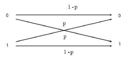
Figure 7-1: Classical noise model

To describe the process mathematically suppose that $\left(p_{0},p_{1}\right)$ and $\left(q_{0},q_{1}\right)$ are the probabilities of bits of being in state $\left(0,1\right)$ before and after the interaction respectively. Therefore, the whole process can be expressed as

$$\left[\begin{array}[]{c}q_{0}\\ q_{1}\end{array}\right]=\left[\begin{array}[]{cc}1-p&p\\ p&1-p\end{array}\right]\left[\begin{array}[]{c}p_{0}\\ p_{1}\end{array}\right],$$ (7.1)

which can be written as

$$\vec{q}=E\vec{p},$$ (7.2)

where $E$ is known as evolution matrix. For any valid probability distribution $\vec{p},$ the evolution matrix $E$ must fulfill the conditions of positivity and completeness. Where the positivity means that all the elements of matrix $E$ are positive and the completeness reflects the fact that the sum of elements in each column of evolution matrix $E$ is one [22].

7.2 Quantum Noise

A quantum system that is totally isolated from unwanted interactions of the outside world is called a closed system; but in real world there is no perfect closed system. For it may suffer from unwanted interactions with the outside world -the environment- that can introduce noise in it. Therefore, such a system is termed as open quantum system. A nice example in this regard is that of a qubit prepared by two positions of an electron that is being interacted by a charge particle acting as a source of uncontrolled noise.

Quantum operations formalism is a mathematical tool that is used to study the behavior of an open system [22]. Let a physical process $\varepsilon$ transform a quantum state $\rho$ as

$$\acute{\rho}=\varepsilon(\rho).$$ (7.3)

For a closed system $\varepsilon$ in Eq. (7.3) is a unitary transformation $U$ and $\varepsilon(\rho)=U\rho U^{\dagger}.$ Whereas the dynamics of an open quantum system is considered to be arising from the interactions of the principal system (system of interest) with the environment and both these systems together form a closed system. Let the principal quantum system be in state $\rho$ and the environment in standard state $\rho_{\text{env}}.$ It is further assumed that system-environment initial state is product state of the form $\rho\otimes\rho_{\text{env}}$ that undergoes a unitary interaction $U$. Then the final state $\acute{\rho}$ of the system is obtained by the relation

$$\acute{\rho}=\varepsilon(\rho)=\mathrm{Tr}_{\text{env}}\left[U\left(\rho\otimes\rho_{\text{env}}\right)U^{\dagger}\right],$$ (7.4)

where $\mathrm{Tr}_{\text{env}}$ represents the partial trace over the environment. In general the final state of the principal system $\varepsilon(\rho)$ may not be related to the initial state by unitary transformation. In the most general case the quantum process $\varepsilon$ is a trace preserving and completely positive linear map that maps the input density matrix to output density matrix [129]. By trace preserving it means that as for the input state $\rho$ it is always true that Tr$\left(\rho\right)=1$ similarly for output state $\acute{\rho}$ it must also be true that Tr$\left(\acute{\rho}\right)=1.$ The positivity condition implies that the quantum process $\varepsilon$ maps the positive density matrix $\rho$ (having non-negative eigenvalues) to positive density matrix $\acute{\rho}.$ To explain complete positivity another system $R$ having density matrix $\rho_{R}$ is introduced so that the initial state of the system becomes $\rho_{R}\otimes\rho.$ Then a map $\varepsilon$ is complete positive if the process $I\otimes\varepsilon$ ($I$ is identity) maps the positive operator $\rho_{R}\otimes\rho$ to positive operator $\rho_{R}\otimes\acute{\rho}.$

For the state of environment $\rho_{\text{env}}=\left|e_{0}\right\rangle\left\langle e_{0}\right|$ with $\left|e_{k}\right\rangle$ as orthonormal basis for the finite dimensional state space of the environment, Eq. (7.4) gives

$$\varepsilon(\rho) = \mathrm{Tr}_{\text{env}}\left[U\left(\rho\otimes\left|e_{0}\right\rangle\left\langle e_{0}\right|\right)U^{\dagger}\right]$$ (7.5)

$$= \mathop{\textstyle\sum}\left\langle e_{k}\right|U\left(\rho\otimes\left|e_{0}\right\rangle\left\langle e_{0}\right|\right)U^{\dagger}\left|e_{k}\right\rangle$$

$$= \mathop{\textstyle\sum}E_{k}\rho E_{k}^{\dagger},$$

where $E_{k}=\left\langle e_{k}\right|U\left|e_{0}\right\rangle$ are Kraus operators acting on the principal system. These operators satisfy the completeness relation

$$\mathop{\textstyle\sum}E_{k}E_{k}^{\dagger}=I,$$ (7.6)

for trace preserving processes and the representation (7.5) is called Kraus representation or operator sum representation for process $\varepsilon.$ It is one of the powerful mathematical representation for quantum operations [22].

7.3 Quantum Correlated Noise

One of the important examples of quantum noise is decoherence that is a non-unitary dynamics and results due to the coupling of principal system with the environment. Decoherence in form of phase damping or dephasing is much interesting. It is uniquely quantum mechanical and describes the loss of quantum information without loss of energy. The energy eigenstate of the system do not change as a function of time during this process but the system accumulates a phase proportional to the eigenvalue. With the passage of time the relative phase between the energy eingenstates may be lost. In pure dephasing process a qubit transforms as

$$a\left|0\right\rangle+b\left|1\right\rangle\rightarrow a\left|0\right\rangle+be^{i\phi}\left|1\right\rangle,$$ (7.7)

where $\phi$ is the phase kick. If this phase kick, $\phi$ is assumed to be a random variable with Gaussian distribution of mean zero and variance $2\lambda$ then the density matrix of system after averaging over all the values of $\phi$ is [22]

$$\left[\begin{array}[]{cc}\left|a\right|^{2}&ab^{\ast}\\ a^{\ast}b&\left|b\right|^{2}\end{array}\right]\rightarrow\left[\begin{array}[]{cc}\left|a\right|^{2}&ab^{\ast}e^{-\lambda}\\ a^{\ast}be^{-\lambda}&\left|b\right|^{2}\end{array}\right].$$ (7.8)

It is evident from the above equation that in this process the phase kicks cause the off-diagonal elements of the density matrix to decay exponentially to zero with time. Which means that a quantum system initially prepared in a pure state

$$a\left|0\right\rangle+b\left|1\right\rangle$$ (7.9)

decays to in an incoherent superposition of states of the form

$$\left|a\right|^{2}\left|0\right\rangle\left\langle 0\right|+\left|b\right|^{2}\left|1\right\rangle\left\langle 1\right|$$ (7.10)

In the operator sum representation the dephasing process can be expressed as [22, 92]

$$\rho_{f}=\overset{1}{\underset{i=0}{\mathop{\textstyle\sum}}}A_{i\text{ }}\rho_{\text{in}}A_{i}^{\dagger},$$ (7.11)

where 

$$A_{0} = \sqrt{1-\frac{p}{2}}I,$$

$$A_{1} = \sqrt{\frac{p}{2}}\sigma_{z},$$ (7.12)

are the Kraus operators,$\ I$ is the identity operator and $\sigma_{z}$ is the Pauli matrix. Recognizing $1-p=e^{-\lambda},$ let $N$ qubits are allowed to pass through such a channel then Eq. (7.11) becomes

$$\rho_{f}=\overset{N}{\underset{k_{1},\text{ ...,\ }k_{n}=0}{\mathop{\textstyle\sum}}}\left(A_{k_{n}}\otimes......A_{k_{1}}\right)\rho_{\text{in }}\left(A_{k_{1}}^{\dagger}\otimes......A_{k_{n}}^{\dagger}\right).$$ (7.13)

Now if noise is correlated with memory of degree $\mu,$ the Kraus operators for two qubit system become [140]

$$A_{i,j}=\sqrt{p_{i}\left[\left(1-\mu\right)p_{j}+\mu\delta_{ij}\right]}A_{i}\otimes A_{j}.$$ (7.14)

Physically, this expression means that with the probability $1-\mu$ the noise is uncorrelated and can be completely specified by the Kraus operators $A_{i,j}^{u}=\sqrt{p_{i}p_{j}}A_{i}\otimes A_{j}$ whereas with probability $\mu$ the noise is correlated and is specified by Kraus operators of the form $A_{ii}^{c}=\sqrt{p_{i}}A_{i}\otimes A_{i}.$

7.4 Quantization of Games in Presence of Correlated Noise

The protocol for quantum games in presence of decoherence is developed by Flitney and Abbott [128]. An initial entangled state is prepared by the arbiter and passed on to the players through a dephasing quantum channel. On receiving the quantum state players apply their local operators (strategies) and return it back to arbiter again through a dephasing quantum channel. Then arbiter performs the measurement and announces their payoffs.

The initial quantum state of game is given by Eq. (6.6) and the strategies of the players are given by Eq. (6.7) with unitary operators $R_{i}$, $P_{i}$ defined as:

$$R_{i}\left|0\right\rangle =e^{i\phi_{i}}\left|0\right\rangle,\text{ \ \ }R_{i}\left|1\right\rangle=e^{-i\phi_{i}}\left|1\right\rangle,$$

$$P_{i}\left|0\right\rangle =e^{i\left(\frac{\pi}{2}-\psi\right)}\left|1\right\rangle,\text{ \ \ \ \ \ }P_{i}\left|1\right\rangle=e^{i\left(\frac{\pi}{2}+\psi\right)}\left|0\right\rangle,$$ (7.15)

where $-\pi\leq\phi_{i},\psi_{i}\leq\pi.$ This is extension of generalized quantization scheme to three strategy set of parameters in accordance with Ref. [29]. The payoff operators used by the arbiter to determine the payoff for Alice and Bob are

$$P=\$_{00}P_{00}+\$_{01}P_{01}+\$_{10}P_{10}+\$_{11}P_{11},$$ (7.16)

where for $m,n=0,1$ operators $P_{mn}=\left|\psi_{mn}\right\rangle\left\langle\psi_{mn}\right|$ are explained in Eqs. (6.14) with $\delta\in\left[0,\frac{\pi}{2}\right]$ and $\$_{ij}$ are the elements of payoff matrix in $ith$ row and $jth$ column . As stated in section (6.2) these operators reduce to that of Eisert’s scheme for $\delta$ equal to $\gamma,$ which represents the entanglement of the initial state [27]. And for $\delta=0$ above operators transform into that of Marinatto and Weber’s scheme [28]. Using Eqs. (6.6), (9.8), (7.14) and (7.16) the payoffs come out to be

$$\$(\theta_{i},\phi_{i},\psi_{i}) = c_{1}c_{2}\left[\eta\$_{00}+\chi\$_{11}+\left(\$_{00}-\$_{11}\right)\mu_{p}^{(1)}\mu_{p}^{(2)}\xi\cos 2(\phi_{1}+\phi_{2})\right]$$

$$+s_{1}s_{2}\left[\eta\$_{11}+\chi\$_{00}-\left(\$_{00}-\$_{11}\right)\mu_{p}^{(1)}\mu_{p}^{(2)}\xi\cos 2(\psi_{1}+\psi_{2})\right]$$

$$+c_{1}s_{2}\left[\eta\$_{01}+\chi\$_{10}+\left(\$_{01}-\$_{10}\right)\mu_{p}^{(1)}\mu_{p}^{(2)}\xi\cos 2(\phi_{1}-\psi_{2})\right]$$

$$+c_{2}s_{1}\left[\eta\$_{10}+\chi\$_{01}-\left(\$_{01}-\$_{10}\right)\mu_{p}^{(1)}\mu_{p}^{(2)}\xi\cos 2(\phi_{2}-\psi_{1})\right]$$

$$+\frac{\mu_{p}^{(2)}\left(\$_{00}-\$_{11}\right)}{4}\sin\theta_{1}\sin\theta_{2}\sin\delta\sin\left(\phi_{1}+\phi_{2}+\psi_{1}+\psi_{2}\right)$$

$$+\frac{\mu_{p}^{(2)}\left(\leavevmode\hbox{\hbox to0.0pt{\thinspace/\hss}{$\$$}}_{10}-\$_{01}\right)}{4}\sin\theta_{1}\sin\theta_{2}\sin\delta\sin\left(\phi_{1}-\phi_{2}+\psi_{1}-\psi_{2}\right)$$

$$+\frac{\mu_{p}^{(1)}\left(-\$_{00}-\$_{11}+\$_{01}+\$_{10}\right)}{4}\sin\theta_{1}\sin\theta_{2}\sin\gamma\sin\left(\phi_{1}+\phi_{2}-\psi_{1}-\psi_{2}\right),$$

where

$$\eta = \cos^{2}\left(\delta/2\right)\cos^{2}\left(\gamma/2\right)+\sin^{2}\left(\delta/2\right)\sin^{2}\left(\gamma/2\right),$$

$$\chi = \cos^{2}\left(\delta/2\right)\sin^{2}\frac{\gamma}{2}+\sin^{2}\left(\delta/2\right)\cos^{2}\left(\gamma/2\right),$$

$$\xi = 1/2\left(\sin\delta\sin\gamma\right),$$

$$c_{i} = \cos^{2}\frac{\theta_{i}}{2},$$

$$s_{i} = \sin^{2}\frac{\theta_{i}}{2},$$

$$\mu_{p}^{(i)} = \left(1-\mu_{i}\right)\left(1-p_{i}\right)^{2}+\mu_{i}.$$

The payoff for the players can be found by putting the appropriate values for $\$_{ij}$ (elements of the payoff matrix for the corresponding game) in Eq. (LABEL:payoff_correlated). These payoffs become the classical payoffs for $\delta=\gamma=0$ and for $\delta=\gamma=\frac{\pi}{2}$and $\mu=0$ these payoffs transform to the results of Flitney and Abbott [128]. It is known that decoherence has no effect on the Nash equilibrium of the game but it causes a reduction in the payoffs [127, 128]. In our case it is interesting to note that this reduction of the payoffs depends on the degree of memory $\mu.$ As $\mu$ increases from zero to one the effect of noise reduces until finally for $\mu=1$ the payoffs become as that for noiseless game irrespective of any value of $p_{i}$. It is further to be noted that in comparison to memoryless case [128] the quantum phases $\phi_{i},\psi_{i}$ do not vanish even for maximum value of decoherence, i.e.,. for $p_{1}=p_{2}=1$.

To see further the effects of memory in quantum games we consider a situation in which Alice is restricted to play classical strategies, i.e., $\phi_{1}=\psi_{1}=0,$ whereas Bob is capable of playing the quantum strategies as well. Under these circumstances following four cases for the different combinations of $\delta$ and $\gamma$ are worth noting:

Case (i) When $\delta=\gamma=0$ then it is clear from Eq. (LABEL:payoff_correlated) payoffs  are the same as in the case of classical game [72]. These payoffs, as expected, are independent of the dephasing probabilities $p_{i}$, the quantum strategies $\phi_{2},\psi_{2}$ and the memory.

Case (ii) When $\delta=0,\gamma\neq 0$ then $\eta=\cos^{2}\frac{\gamma}{2},\chi=\sin^{2}\frac{\gamma}{2},$and $\xi=0.$ Using payoff matrix (2.3) for the game of Prisoners’ Dilemma and Eq. (LABEL:payoff_correlated) the payoffs for the two players are:

$$\$^{A}(\theta_{1},\theta_{2},\phi_{2},\psi_{2}) = c_{1}c_{2}\left(3-2\sin^{2}\frac{\gamma}{2}\right)+s_{1}s_{2}\left(1+2\sin^{2}\frac{\gamma}{2}\right)$$

$$+5c_{1}s_{2}\sin^{2}\frac{\gamma}{2}+5c_{2}s_{1}\left(1-\sin^{2}\frac{\gamma}{2}\right)$$

$$+\frac{\mu_{p}^{(1)}}{4}\sin\theta_{1}\sin\theta_{2}\sin\gamma\sin\left(\phi_{2}-\psi_{2}\right),$$

$$\$^{B}(\theta_{1},\theta_{2},\phi_{2},\psi_{2}) = c_{1}c_{2}\left(3-2\sin^{2}\frac{\gamma}{2}\right)+s_{1}s_{2}\left(1+2\sin^{2}\frac{\gamma}{2}\right)$$ (7.18)

$$+5c_{1}s_{2}\left(1-\sin^{2}\frac{\gamma}{2}\right)+5c_{2}s_{1}\sin^{2}\frac{\gamma}{2}$$

$$+\frac{\mu_{p}^{(1)}}{4}\sin\theta_{1}\sin\theta_{2}\sin\gamma\sin\left(\phi_{2}-\psi_{2}\right).$$

In this case the optimal strategy for the quantum player, Bob, is $\phi_{2}-\psi_{2}=\frac{\pi}{2}.$ Though his choice for $\theta_{2}$ depends on Alice’s choice for $\theta_{1},$but he can play $\theta_{2}=\frac{\pi}{2},$ without being bothered about Alice’s choice as rational reasoning leads Alice to play $\theta_{1}=\frac{\pi}{2}$. Under these choices of moves the payoffs for the two players are equal:

$$\$^{A}(\frac{\pi}{2},\frac{\pi}{2},\phi_{2}-\psi_{2} = \frac{\pi}{2})=\$^{B}(\frac{\pi}{2},\frac{\pi}{2},\phi_{2}-\psi_{2}=\frac{\pi}{2})$$ (7.19)

$$= \frac{9}{4}+\frac{\mu_{p}^{(1)}}{4}\sin\gamma.$$

It is evident that the quantum player has no advantage over the classical player. Similarly for the Chicken game putting the payoffs from payoff matrix (2.5) we get:

$$\$^{A}(\theta_{1},\theta_{2},\phi_{2},\psi_{2}) = c_{1}c_{2}\left(3-3\sin^{2}\frac{\gamma}{2}\right)+s_{1}s_{2}\left(3\sin^{2}\frac{\gamma}{2}\right)$$ (7.20)

$$+c_{1}s_{2}\left(3\sin^{2}\frac{\gamma}{2}+1\right)+c_{2}s_{1}\left(4-3\sin^{2}\frac{\gamma}{2}\right)$$

$$+\frac{\mu_{p}^{(1)}}{2}\sin\theta_{1}\sin\theta_{2}\sin\gamma\sin\left(\phi_{2}-\psi_{2}\right),$$

$$\$^{B}(\theta_{1},\theta_{2},\phi_{2},\psi_{2}) = c_{1}c_{2}\left(3-3\sin^{2}\frac{\gamma}{2}\right)+s_{1}s_{2}\left(3\sin^{2}\frac{\gamma}{2}\right)$$ (7.21)

$$+c_{1}s_{2}\left(4-3\sin^{2}\frac{\gamma}{2}\right)+c_{2}s_{1}\left(1+3\sin^{2}\frac{\gamma}{2}\right)$$

$$+\frac{\mu_{p}^{(1)}}{2}\sin\theta_{1}\sin\theta_{2}\sin\gamma\sin\left(\phi_{2}-\psi_{2}\right),$$

and it can be shown using the same argument as for the game of Prisoners’ Dilemma that the quantum player does not have any advantage over classical player in the Chicken game as well.

For the case of the quantum Battle of Sexes using values from payoff matrix (2.6) the payoffs become

$$\$^{A}(\theta_{1},\theta_{2},\phi_{2},\psi_{2}) = c_{1}c_{2}\left(2-\sin^{2}\frac{\gamma}{2}\right)+s_{1}s_{2}\left(1+\sin^{2}\frac{\gamma}{2}\right)$$

$$-\frac{3\mu_{p}^{(1)}}{4}\sin\theta_{1}\sin\theta_{2}\sin\gamma\sin\left(\phi_{2}-\psi_{2}\right),$$

$$\$^{B}(\theta_{1},\theta_{2},\phi_{2},\psi_{2}) = c_{1}c_{2}\left(1+\sin^{2}\frac{\gamma}{2}\right)+s_{1}s_{2}\left(2-\sin^{2}\frac{\gamma}{2}\right)$$ (7.22)

$$-\frac{3\mu_{p}^{(1)}}{4}\sin\theta_{1}\sin\theta_{2}\sin\gamma\sin\left(\phi_{2}-\psi_{2}\right).$$

Here the optimal strategy for Bob is $\phi_{2}-\psi_{2}=-\frac{\pi}{2}$ and $\theta_{2}=\frac{\pi}{2}$, keeping in view that the best strategy for Alice is $\theta_{1}=\frac{\pi}{2}.$ The corresponding payoffs of the players are again equal for these choices, i.e.,

$$\$^{A}(\frac{\pi}{2},\frac{\pi}{2},\phi_{2}-\psi_{2} = -\frac{\pi}{2})=\$^{B}(\frac{\pi}{2},\frac{\pi}{2},\phi_{2}-\psi_{2}=-\frac{\pi}{2})$$ (7.23)

$$= \frac{3}{4}+\frac{3}{4}\mu_{p}^{(1)}\sin\gamma.$$

It is clear that for the case $\delta=0,\gamma\neq 0$ the quantum player has no advantage over the classical player for three games considered above. It is interesting because the game starts from an entangled state and the payoffs are also the functions of the quantum phases, $\phi_{i},\psi_{i},$ dephasing probability, $p_{1}$ and the degree of memory, $\mu_{1}$, of the quantum channel between Bob and arbiter.

Case (iii) When $\delta\neq 0,\gamma=0$ then using Eq. (LABEL:payoff_correlated) and the values from the payoff matrices given in subsection (2.3) the payoffs for the two players in games of Prisoners’ Dilemma, Chicken and Battle of Sexes are

$$\$^{A}(\theta_{1},\theta_{2},\phi_{2},\psi_{2}) = c_{1}c_{2}\left(3-2\sin^{2}\frac{\delta}{2}\right)+s_{1}s_{2}\left(1+2\sin^{2}\frac{\delta}{2}\right)$$

$$+\frac{7\mu_{p}^{(2)}}{4}\sin\theta_{1}\sin\theta_{2}\sin\delta\sin\left(\phi_{2}+\psi_{2}\right),$$

$$\$^{B}(\theta_{1},\theta_{2},\phi_{2},\psi_{2}) = c_{1}c_{2}\left(1+\sin^{2}\frac{\delta}{2}\right)+s_{1}s_{2}\left(2-\sin^{2}\frac{\delta}{2}\right)$$ (7.24)

$$-\frac{3\mu_{p}^{(2)}}{4}\sin\theta_{1}\sin\theta_{2}\sin\delta\sin\left(\phi_{2}+\psi_{2}\right),$$

$$\$^{A}(\theta_{1},\theta_{2}) = c_{1}c_{2}\left(3-3\sin^{2}\frac{\delta}{2}\right)+s_{1}s_{2}\left(3\sin^{2}\frac{\delta}{2}\right)+c_{1}s_{2}\left(1+3\sin^{2}\frac{\delta}{2}\right)$$

$$+c_{2}s_{1}\left(4-3\sin^{2}\frac{\delta}{2}\right),$$

$$\$^{B}(\theta_{1},\theta_{2},\phi_{2},\psi_{2}) = c_{1}c_{2}\left(3-3\sin^{2}\frac{\delta}{2}\right)+s_{1}s_{2}\left(3\sin^{2}\frac{\delta}{2}\right)+c_{1}s_{2}\left(4-3\sin^{2}\frac{\delta}{2}\right)$$

$$+c_{2}s_{1}\left(1+3\sin^{2}\frac{\delta}{2}\right)+\frac{3\mu_{p}^{(2)}}{2}\sin\theta_{1}\sin\theta_{2}\sin\delta\sin\left(\phi_{2}+\psi_{2}\right),$$

and

$$\$^{A}(\theta_{1},\theta_{2},\phi_{2},\psi_{2}) = c_{1}c_{2}\left(2-\sin^{2}\frac{\delta}{2}\right)+s_{1}s_{2}\left(1+\sin^{2}\frac{\delta}{2}\right)$$

$$+\frac{3\mu_{p}^{(2)}}{4}\sin\theta_{1}\sin\theta_{2}\sin\delta\sin\left(\phi_{2}+\psi_{2}\right),$$

$$\$^{B}(\theta_{1},\theta_{2},\phi_{2},\psi_{2}) = c_{1}c_{2}\left(1+\sin^{2}\frac{\delta}{2}\right)+s_{1}s_{2}\left(2-\sin^{2}\frac{\delta}{2}\right)$$ (7.26)

$$-\frac{3\mu_{p}^{(2)}}{4}\sin\theta_{1}\sin\theta_{2}\sin\delta\sin\left(\phi_{2}+\psi_{2}\right),$$

respectively. It is evident from the above expressions for the payoffs that the optimal strategy for Bob, the quantum player, is $\phi_{2}+\psi_{2}=-\frac{\pi}{2}$ with, $\theta_{2}=\frac{\pi}{2},$for Prisoners’ Dilemma and Battle of Sexes. But corresponding payoff for Alice is less. However, she can overcome this by playing $\theta_{1}=0$ or $\pi,$ so that the payoffs for both the players become independent of the quantum phases $\phi_{2},\psi_{2}$. So there remain no option for the quantum player to enhance his payoff by exploiting the quantum move. However in the case of Chicken game the quantum player can enhance his payoff without effecting the payoff of classical player. But again the classical player has the ability to prevent quantum strategies by playing $\theta_{1}=0$ or $\pi.$ So there remains no advantage for playing quantum strategies. It is also interesting to note that though by playing this move Alice could force the payoffs of the two players to be independent of dephasing factor $p_{2}$ and the degree of memory $\mu_{2}$, however, the game remains different from its classical counterpart.

Case (iv) When $\delta=\gamma=\frac{\pi}{2},$then Eq. (LABEL:payoff_correlated) with $\mu_{1}=\mu_{2}=0,$ gives the results of Flitney and Abbott [128] and the quantum player is better off for $p<1$. However, when decoherence increases this advantage diminishes and vanishes for maximum decoherence, i.e., $p=1$. But in our case when $\mu\neq 0$, the quantum player is always better off even for maximum noise, i.e., $p=1,$ which was not possible in memoryless case. Furthermore it is worth noting that as the degree of memory increases from $0$ to $1$ the effect of noise on the payoffs starts decreasing and for $\mu=1$ it behaves like a noiseless game.

In the case of Prisoners’ Dilemma, the optimal strategy for Bob is to play $\phi_{2}=\frac{\pi}{2}$ and $\psi_{2}=0.$ His choice for, $\theta_{2},$ is $\frac{\pi}{2}$, independent of Alice’s move. The payoffs for Alice and Bob as a function of decoherence probability $p_{1}=p_{2}=p$ at $\mu=\frac{1}{2},$ is

$$\$^{A}(\theta_{1},\theta_{2},\phi_{2},\psi_{2}) = c_{1}c_{2}\left[2+\mu_{p}^{2}\cos 2\phi_{2}\right]+s_{1}s_{2}\left[2-\mu_{p}^{2}\cos 2\psi_{2}\right]$$

$$+\frac{5}{2}c_{1}s_{2}\left[1-\mu_{p}^{2}\cos 2\psi_{2})\right]+\frac{5}{2}c_{2}s_{1}\left[1+\mu_{p}^{2}\cos 2\phi_{2}\right]$$

$$+\frac{\mu_{p}}{4}\sin\theta_{1}\sin\theta_{2}\sin\left(\phi_{2}-\psi_{2}\right)-\frac{3\mu_{p}}{4}\sin\theta_{1}\sin\theta_{2}\sin\left(\phi_{2}+\psi_{2}\right),$$

$$\$^{B}(\theta_{1},\theta_{2},\phi_{2},\psi_{2}) = c_{1}c_{2}\left[2+\mu_{p}^{2}\cos 2\phi_{2}\right]+s_{1}s_{2}\left[2-\mu_{p}^{2}\cos 2\psi_{2}\right]$$

$$+\frac{5}{2}c_{1}s_{2}\left[1+\mu_{p}^{2}\cos 2\psi_{2}\right]+\frac{5}{2}c_{2}s_{1}\left[1-\mu_{p}^{2}\cos 2\phi_{2}\right]$$

$$+\frac{7\mu_{p}}{4}\sin\theta_{1}\sin\theta_{2}\sin\left(\phi_{2}+\psi_{2}\right)+\frac{\mu_{p}}{4}\sin\theta_{1}\sin\theta_{2}\sin\left(\phi_{2}-\psi_{2}\right),$$

where

$$\mu_{p}=\frac{1+\left(1-p\right)^{2}}{2}.$$

It is obvious from above payoffs that quantum player Bob can always out perform Alice, for all values of $p$. Similarly for the case of Chicken and Battle of Sexes game, it can be proved that the classical player can be out performed by Bob, at $\phi_{2}=\frac{\pi}{2},\psi_{2}=0$ and $\theta_{2}=\frac{\pi}{2}$ and $\phi_{2}=-\frac{\pi}{2},\psi=0$ and $\theta_{2}=\frac{\pi}{2},$ respectively.

7.5 Summary

Quantum games with correlated noise are studied under the generalized quantization scheme with three parameter set of strategies. Three games, Prisoners’ Dilemma, Battle of Sexes and Chicken game are studied with one player restricted to classical strategy while other allowed to play quantum strategies. It is shown that the effects of the memory and decoherence become effective for the case, $\gamma=\delta=\frac{\pi}{2},$ for which quantum player out perform classical player. It is also shown that memory controls payoffs reduction due to decoherence and for the limit of maximum memory decoherence becomes ineffective.

Chapter 8 Quantum Key Distribution

Cryptography is the science of secret communication. Over the centuries it developed from the protocols of simple transposition and substitution to modern cryptographic schemes like one-time pads and public key cryptosystems [130, 131, 96]. All of these schemes rely on a secret key that is shared between the sender and intended receiver prior to any secure communication between them. However, the security of the key can never be ensured and if it becomes known then any one can decrypt the message. In one-time pads protocol, for example, the sender and receiver physically exchange the key and store it at some secure location. In such an exchange the key can be copied either during the exchange or from the secure location. In public key cryptosystems, such as, RSA, the receiver generates a pair of keys: a public key and a private key [96]. The security of the communication relies on determining the prime factors of a large integer. It is generally believed that the number of steps a classical computer would need to factorize an N decimal digit, grows exponentially with N. With recent advances in quantum computing, it is now possible to factorize very large numbers much faster. As a result the security of RSA will be at risk. This problem can easily be fixed by quantum cryptography.

Quantum cryptography offers an entirely new technique for secure key distribution where security relies upon the laws of quantum physics instead of computational complexity. There are two different protocols for quantum cryptography: one developed by Bennett et al. [98, 99, 97] which is based on the no-cloning theorem and the uncertainty principle; while the other was presented by Ekert [38] which involves quantum entanglement and the violation of Bell’s theorem [132]. In this protocol the Bell’s inequalities are used to detect the presence of Eve to ensure secure key distribution. Quantum cryptography can also be thought of as a game between the sender and receiver, who want to communicate, and the eavesdroppers [38]. In this chapter we present a new protocol for quantum key distribution based on quantum game theory. Here the disturbance in predefined values of the elements of a decoding matrix (payoff matrix) detects the presence of Eve.

8.1 Classical Cryptography

The important and widely used protocols of classical cryptography are one-time pads and RSA public cryptography. Next we introduce them one by one.

8.1.1 One-Time Pads

Despite of being secure it is one of the simplest cryptosystems. It is rumored that it remained in use for communicating diplomatic information between Washington and Moscow [95]. In this cryptosystem, prior to any communication, Alice and Bob who are interested in secret communication meet in a safe place and share a large number of secret keys printed in form of booklets or pads. The keys are random numbers picked uniformly in the range $0$ to $l-1$, where $l$ is the number of symbols in the alphabet. Then they return home with the pad of keys in their possession.

When Alice wants to convey a secret message to Bob she follows the following steps.

1. The message $M_{text}$ consisting of $N$ symbols is converted to a sequence of $N$ integers $M=\left\{m_{1},m_{2},....,m_{N}\right\}$.

2. A key $K=\left\{k_{1},k_{2},.....,k_{N}\right\}$ is selected from a page $P$ of her secret key pad shared with Bob.

3. The message $M$ is encrypted to $E=\left\{e_{1},e_{2},....,e_{N}\right\}$ using formula

   $$e_{i}=m_{i}+k_{i}\mathop{\mathrm{m}od}l,$$

   where $l$ is the number of symbols in the alphabet.

4. The encrypted message $E$ along with keys pad page $P\$i.e. $\left(E,P\right)$ is sent to Bob.

Bob on receiving the message performs the following steps.

1. The message $M=\left\{m_{1},m_{2},....,m_{N}\right\}$ is decrypted by taking the key $K=\left\{k_{1},k_{2},.....,k_{N}\right\}$ used by Alice from page $P$ of the shared key pads and the relation

   $$m_{i}=e_{i}-k_{i}+l\mathop{\mathrm{m}od}l.$$

2. The message is converted back to $M_{text}$ from this sequence of integers.

8.1.2 RSA Public Cryptography

This cryptosystem was invented by Ronald Rivest, Adi Shamir and Leonard Adleman hence it bears the name RSA cryptosystem [96]. In this protocol a person wishing to receive secret messages creates a pair of keys known as public key and private key. The public key is publicized but the private key is kept secret. If somebody is interested in sending secret message he takes the public key of the intended recipient to encrypt the message. Upon receiving the scrambled message the receiver decrypts it with the help of his private key. In the following we give the mathematical details required to know how the keys are generated and how the messages are encrypted and decrypted.

In order to generate the public and private keys the receiver takes two large prime numbers $p,q$ and finds their product $n=pq.$ Next he finds an integer $d$ that is coprime to $(1-p)(1-q),$ and computes $e$ with the help of the relation

$$ed\equiv 1\mathop{\mathrm{m}od}(1-p)(1-q).$$ (8.1)

The public key to be broadcasted is a pair of numbers $(e,n)$ and the private key is the pair of numbers $(d,n).$ The interested party in sending secret messages converts the text $M_{text}$ to a sequence of integers, $M_{i}$ and then encrypts it by the use of the following formula

$$E_{i}=\left(M_{i}\right)^{e}\mathop{\mathrm{m}od}n.$$ (8.2)

On reception the receiver decrypts this message using

$$M_{i}=\left(E_{i}\right)^{d}\mathop{\mathrm{m}od}n,$$ (8.3)

and then converts it back to original text.

To break the code in RSA cryptosystem one requires the private key, $(d,n)$ with the help of public key, $(e,n).$ That can be accomplished very easily with the help of equation (8.1) subject to the condition if one can find the prime factors of $n.$i.e. the prime numbers $p$ and $q$. But it is believed that performing prime factorization of a very large number is difficult by any classical computer. Therefore, RSA is secure. However with the advent of quantum computer it will not remain difficult to find prime factors of large numbers hence RSA cryptosystem will not remain secure. At that time we will need quantum cryptography.

8.2 Quantum Cryptography

In the next we explain two simple protocols that utilize two different quantum phenomenon to protect the secret information from being tampered.

8.2.1 BB84 Protocol

This protocol was introduced by Charles H. Bennett and Gilles Brassard in 1984 hence it bears the name BB84 [98]. Security in this protocol relies on the inability to measure non-orthogonal quantum states perfectly. The task is accomplished by coding logical bit 0 into two different non-orthogonal quantum states and similarly 1 into two other non-orthogonal states such that the encoding states for 0 and 1 are pairwise orthogonal.

Let the information be encoded into polarization states of individual photons such that

$$0 \longrightarrow \left\{\begin{array}[]{c}\left|H\right\rangle\\ \left|A\right\rangle=\frac{\left|H\right\rangle+\left|V\right\rangle}{\sqrt{2}}\end{array}\right.,$$ (8.6)

$$1 \longrightarrow \left\{\begin{array}[]{c}\left|V\right\rangle\\ \left|D\right\rangle=\frac{\left|H\right\rangle-\left|V\right\rangle}{\sqrt{2}}\end{array}\right.,$$ (8.9)

where $\left|H\right\rangle$ and $\left|V\right\rangle$ represent the horizontal and vertical polarizations of a photon respectively. The states $\left|H\right\rangle$ and $\left|V\right\rangle$ are also termed as rectilinear bases where as the states $\left|A\right\rangle$ and $\left|D\right\rangle$ are called diagonal bases.

It can be seen from Eq. (8.9) that the four polarization states are pairwise orthogonal i.e.

$$\left\langle V\right.\left|H\right\rangle=\left\langle A\right.\left|D\right\rangle=0.$$ (8.10)

Furthermore if the measurement is performed in bases identical to the bases in which a photon is prepared it gives deterministic results otherwise random outcomes are achieved i.e.

$$\left\langle H\right.\left|H\right\rangle = \left\langle V\right.\left|V\right\rangle=\left\langle A\right.\left|A\right\rangle=\left\langle D\right.\left|D\right\rangle=1,$$

$$\left|\left\langle H\right.\left|A\right\rangle\right|^{2} = \left|\left\langle H\right.\left|D\right\rangle\right|^{2}=\left|\left\langle V\right.\left|A\right\rangle\right|^{2}=\left|\left\langle V\right.\left|D\right\rangle\right|^{2}=\frac{1}{2}.$$

Prior to any key distribution Alice and Bob agree that $\left|H\right\rangle$ and $\left|A\right\rangle$ stand for bit value $0$ whereas $\left|V\right\rangle$ and $\left|D\right\rangle$ stand for $1$. Then the sender, Alice generates a sequence of random numbers and encodes them using the predefined four polarization states. The polarization states for coding are used randomly and independently. Upon receiving the photons Bob performs the measurements using the rectilinear or diagonal bases randomly and independently of Alice. Statistically their bases match in about 50% cases which gives Bob deterministic results. Then they contact on a public channel and tell each other which bases they have used. Whenever their bases coincide they record the results otherwise they discard it. In case there is no eavesdropper in the channel then Bob receives the same bit that Alice has transmitted.

If there is an eavesdropping, Eve in the way from Alice to Bob who performs measurements in the bases similar to Bob to see what bits are being sent. She intercepts the photon chooses the bases randomly and performs the measurement to decode the bit. In order to remain hidden from Alice and Bob sight Eve will transmit the photon in same polarization state in which she received it. In this situation she will make an error for quarter of the time. But in this scenario for the cases where the bases of Alice and Bob match the results of Alice and Bob will not be correlated which uncovers the presence of Eve so they abort communication.

8.2.2 Ekert Protocol

This protocol was presented by Artur Ekert [13] in 1991. It works as follows: Alice and Bob share a large number of two qubit entangled states of the form

$$\left|\psi\right\rangle=\frac{\left|01\right\rangle-\left|10\right\rangle}{\sqrt{2}}.$$ (8.11)

In order to share secret key Alice and Bob perform measurements on their respective qubits. Let they, for example, perform measurement on their qubits at angles of $\left\{0^{\circ},45^{\circ},90^{\circ}\right\}$ and $\left\{45^{\circ},90^{\circ},135^{\circ}\right\}$ respectively in a plane perpendicular to axis connecting them. The sequence of these measurements are performed in complete random way. However for the choice of same orientations of their detector and in case there is no eavesdropping in the way then their results are always totally anticorrelated. On the other hand when the orientations of their detectors do not match then quantum mechanics tells the way for the calculation of correlation coefficient. In this case if $P_{\pm\mp}\left(\theta_{i}^{a},\theta_{j}^{b}\right)$ is the probability of getting spin up (+1) and spin down (-1) then the correlation coefficient $E\left(\theta_{i}^{a},\theta_{j}^{b}\right)$ is found as

$$E\left(\theta_{i}^{a},\theta_{j}^{b}\right)=P_{++}\left(\theta_{i}^{a},\theta_{j}^{b}\right)+P_{--}\left(\theta_{i}^{a},\theta_{j}^{b}\right)-P_{+-}\left(\theta_{i}^{a},\theta_{j}^{b}\right)-P_{-+}\left(\theta_{i}^{a},\theta_{j}^{b}\right)$$ (8.12)

With the help of Eq. (8.12) we can find a function

$$S=E\left(\theta_{1}^{a},\theta_{3}^{b}\right)+E\left(\theta_{1}^{a},\theta_{2}^{b}\right)+E\left(\theta_{2}^{a},\theta_{3}^{b}\right)-E\left(\theta_{2}^{a},\theta_{2}^{b}\right)$$ (8.13)

This function $S$ was proposed by Clauser, Horne, Shimony and Holt for the generalized Bell theorem, known as CHSH inequality [133]. Quantum mechanics demands that

$$S=-2\sqrt{2}$$ (8.14)

After the measurements have been performed then Alice and Bob contact on a public channel to know what orientations of their detectors they have used. They divide these results into two groups. The first group corresponds to the results where they used different orientations of their detectors and the second group belongs the results where they performed the measurement in matching orientations of their detectors. For the first group they announce publicly what results they obtained. Since the orientations of detectors was selected randomly and independently therefore, the correlation between their results according to the principles of quantum mechanics and in the absence of eavesdropping should come out to be $-2\sqrt{2}$ [133]. This assures the legitimate users that the results they obtained in the second group, where they selected the same orientations of the detectors, are totally anticorrelated and can be converted into a secret key. However if Alice and Bob find a significant departure from the expected correlations, that quantum mechanics demands, it indicates the presence of eavesdropper. So they will have to abort the communication. Experimental demonstration of this protocol has been accomplished by Rariry et al. in 1994 [134].

In the next section we present a new scheme for Quantum Key Distribution (QKD) based on the mathematical frame work of our Generalized Quantization Scheme for Games.

8.3 A New Scheme for Quantum Key Distribution

This new scheme for Quantum Key Distribution (QKD) is derived from the quantum game theoretic setup. In fact it is not a quantum game anymore as there is no strategic competition between the two players, Alice and Bob. Alice and Bob shares multiple copies of maximally entangled states. As a first step, Alice and Bob identify a set of unitary operators to code various symbols that needs to be communicated. Then Bob simulates all mutually agreed upon operators of Alice against his choices, at his end and evaluates the expectation values of all decoding operators and constructs a decoding bi-matrix. Bob chooses his operators with the consideration to avoid any overlap among the various expectation values of bi-matrix elements. The expectation values depends on the operators used by Alice and Bob. This decoding bi-matrix will later be used to identify the operator used by Alice.

In the second set of the scheme. Alice applies a local unitary operator on her part of the shared entangled qubit and pass it on to Bob. Bob applies his local unitary operator on his part of the qubit. On receiving the Alice’s part of the qubit, Bob evaluates the expectation values of the two decoding operators and compares the pair of expectation values with the already simulated bi-matrix elements. The comparison would reveal the unitary operator used by Alice. Repeating this process Alice and Bob would be able to share a string of bits which could act as key for secret communication.

In this scheme, it is possible for Eve to perform a measurement while transmission of the Alice’s part of the qubit to Bob. However, any such attempt even on some copies of the maximally entangled qubits shared between Alice and Bob would result in the change in the expectation values. A careful choice of the two decoding operators would enable Bob to detect the presence of Eve. Presence of Eve could be communicated back to Alice via any classical channel to ignore that particular attempt.

One peculiar feature of our protocol is the evaluation of expectation values. This requires multiple copies of the qubit to communicate a required symbol. This in principle could effect the efficiency and security of our protocol. Here we show the number of copies required to communicate a symbol with sure detection of presence of Eve.

Consider a situation where Alice intends to send a symbol $m_{1}$ to Bob with whom she shares a maximally entangled state of the form (3.18a). She applies one of the mutually agreed unitary operator, $U_{A}\left(\theta_{A},\alpha_{A},\beta_{A}\right)=I$ on her part of qubit and sends her part to Bob. Lets assume there is Eve who tries to read the transmitted symbol by performing a measurement on Alice’s part of the qubit, in the computational basis $\left|0\right\rangle$, $\left|1\right\rangle$. Eve knows the unitary operators used by Alice as these operators were mutually agreed by Alice and Bob prior to any key generation. But she is unaware of the operators used by Bob and the decoding bi-matrix used by Bob to determine the unitary operator applied by Alice. Upon measurement she would get either $\left|0\right\rangle$ or $\left|1\right\rangle$ with equal probability. In order to remain hidden from the scene Eve, depending on her measurement results, would send either $\left|0\right\rangle$ or $\left|1\right\rangle$ to Bob. If, for example, on receiving the qubits, Bob decides to apply the identity operator $I$ on his part of the entangled qubit, then the final state in his possession would be either $\left|00\right\rangle$ or $\left|11\right\rangle$ with equal probability. Let the expectation value or bi-matrix elements associated with the state $\left|00\right\rangle$ and $\left|11\right\rangle$ be $\left(a,b\right)$ and $\left(c,d\right),$ respectively. According to the requirement of protocol Alice would have to send $n$ copies of qubits to transmit the symbol $m_{1}$. If Eve succeeds in intercepting $i$ copies out of total $n$ copies then the bi-matrix element $\left(a,b\right)$ associated with the state $\left|00\right\rangle$ becomes

$$\left(\alpha_{i},\beta_{i}\right)=\left(\frac{a\left(n-i\right)+ci}{n},\frac{b\left(n-i\right)+di}{n}\right)$$ (8.15)

and the expectation value with including error introduced by Eve would become:

$$f\left(n\right) = \left(\underset{i=0}{\overset{n}{\sum}}P_{i}\alpha_{i},\underset{i=0}{\overset{n}{\sum}}P_{i}\beta_{i}\right)$$ (8.16)

$$= \left(\frac{a+c}{2},\frac{b+d}{2}\right)$$

where

$$P_{i}=\frac{1}{2^{n}}\left(\begin{array}[]{c}n\\ i\end{array}\right)$$ (8.17)

is the probability for binomial distribution. It is interesting to note that the expression (8.16) is independent of $n,$ the number of copies. Comparing the values given in Eq. (8.15) and those already obtained through simulation, Bob can detect the presence of Eve. Now to estimate of the number of copies required to reliably detect the presence of Eve we take the help of standard deviation. By the use of Eq. (8.16) the standard deviation comes out to be

$$\left(\sigma_{1},\sigma_{2}\right) = \left(\sqrt{\underset{i=0}{\overset{n}{\sum}}P_{i}\alpha_{i}^{2}-\left(\underset{i=0}{\overset{n}{\sum}}P_{i}\alpha_{i}\right)^{2}},\sqrt{\underset{i=0}{\overset{n}{\sum}}P_{i}\beta_{i}^{2}-\left(\underset{i=0}{\overset{n}{\sum}}P_{i}\beta_{i}\right)^{2}}\right)$$ (8.18)

$$= \left(\frac{\left(a-c\right)}{2\sqrt{n}},\frac{\left(b-d\right)}{2\sqrt{n}}\right),$$

which is inversely proportional to $\sqrt{n}.$ Standard deviation can be reduced by increasing the number of copies.

8.3.1 The Description of Protocol

Let Alice and Bob share the initial quantum states of the form of Eq. (6.6). The local unitary operators of Alice and Bob derived from our generalized quantization scheme  are represented by Eq. (6.7) with $R$ and $P$ defined as:

$$R_{A}\left|0\right\rangle =e^{i\alpha_{A}}\left|0\right\rangle,\text{ \ }\ \ \ \ \ \ \ \ \ \ \ \text{\ }R_{A}\left|1\right\rangle=e^{-i\alpha_{A}}\left|1\right\rangle,$$

$$P_{A}\left|0\right\rangle =e^{i\left(\frac{\pi}{2}-\beta_{A}\right)}\left|1\right\rangle,\text{ \ \ \ \ \ \ }P_{A}\left|1\right\rangle=e^{i\left(\frac{\pi}{2}+\beta_{A}\right)}\left|0\right\rangle,$$

$$R_{B}\left|0\right\rangle =\left|0\right\rangle,\text{ \ }\ \ \ \ \ \ \ \ \ \ \ \ \ \ \ \ \text{\ }R_{B}\left|1\right\rangle=\left|1\right\rangle,$$

$$P_{B}\left|0\right\rangle =\left|1\right\rangle,\text{ \ \ \ \ }\ \ \ \ \ \ \ \ \ \ \ \ \text{\ }P_{B}\left|1\right\rangle=-\left|0\right\rangle,$$ (8.19)

where $-\pi\leq\alpha_{A},\beta_{A}\leq\pi.$ The operators used by Bob for the measurement are

$$P^{k}=\$_{00}^{k}P_{00}+\$_{01}^{k}P_{01}+\$_{10}^{k}P_{10}+\$_{11}^{k}P_{11},$$ (8.20)

where $k=A,B$ and for $m,n=0,1$ the operators $P_{mn}=\left|\psi_{mn}\right\rangle\left\langle\psi_{mn}\right|$ are given in Eqs. (6.14) with $\delta\in\left[0,\frac{\pi}{2}\right]$ and $\$_{ij}^{k}$ are the elements of coding matrix in $ith$ row and $jth$ column. It is also important to note that Bob chooses the coding matrix on his own will without being known to Alice. Therefore, it will be difficult for Eve to construct the decoding operators of the form of Eq. (8.20).The rationale in choosing this coding matrix is to avoid or to reduce the overlap of the expectation values of the decoding operators. The results of measurements performed by Bob are recorded as

$$\$_{k}(\theta_{i},\alpha_{A},\beta_{A})=\text{Tr}(P^{k}\rho_{f})\text{,}$$ (8.21)

  where Tr represents the trace of a matrix .

The presence of Eve can be modeled as a phase damping channel [22, 128]. The quantum state after the Eve’s measurement transforms to

$$\rho=\overset{2}{\underset{i=0}{\mathop{\textstyle\sum}}}A_{i\text{ }}\rho_{in}\text{ }A_{i}^{\dagger},$$ (8.22)

where $A_{0}=\sqrt{p}\left|0\right\rangle\left\langle 0\right|,$ $A_{1}=\sqrt{p}\left|1\right\rangle\left\langle 1\right|$ and $A_{2}=\sqrt{1-p}\hat{I}$ are the Kraus operators. Using Eqs. (6.6), (8.20), (8.21) and (7.12) we get

$$\$_{k}(\theta_{i},\alpha_{A},\beta_{A}) =c_{1}c_{2}\left[\eta\$_{00}^{k}+\chi\$_{11}^{k}+\left(\$_{00}^{k}-\$_{11}^{k}\right)\mu_{p}\xi\cos 2\alpha_{A}\right]$$

$$+s_{1}s_{2}\left[\eta\$_{11}^{k}+\chi\$_{00}^{k}-\left(\$_{00}^{k}-\$_{11}^{k}\right)\mu_{p}\xi\cos 2\beta_{A}\right]$$

$$+c_{1}s_{2}\left[\eta\$_{01}^{k}+\chi\$_{10}^{k}+\left(\$_{01}^{k}-\$_{10}^{k}\right)\mu_{p}\xi\cos 2\alpha_{A}\right]$$

$$+c_{2}s_{1}\left[\eta\$_{10}^{k}+\chi\$_{01}^{k}-\left(\$_{01}^{k}-\$_{10}^{k}\right)\mu_{p}\xi\cos 2\beta_{A}\right]$$

$$+\left(\frac{\$_{00}^{k}-\$_{11}^{k}+\$_{10}^{k}-\$_{01}^{k}}{4}\right)\mu_{p}\sin\theta_{1}\sin\theta_{2}\sin\delta\sin\left(\alpha_{A}+\beta_{A}\right)$$

$$+\left(\frac{-\$_{00}^{k}-\$_{11}^{k}+\$_{01}^{k}+\$_{10}^{k}}{4}\right)\sin\theta_{1}\sin\theta_{2}\sin\gamma\sin\left(\alpha_{A}-\beta_{A}\right),$$

(8.23)

where we have defined:

$$\eta = \cos^{2}\left(\delta/2\right)\cos^{2}\left(\gamma/2\right)+\sin^{2}\left(\delta/2\right)\sin^{2}\left(\gamma/2\right),$$

$$\chi = \cos^{2}\left(\delta/2\right)\sin^{2}\frac{\gamma}{2}+\sin^{2}\left(\delta/2\right)\cos^{2}\left(\gamma/2\right),$$

$$\xi = 1/2\left(\sin\delta\sin\gamma\right),\text{ }c_{i}=\cos^{2}\frac{\theta_{i}}{2},$$

$$s_{i} = \sin^{2}\frac{\theta_{i}}{2},\text{ }\mu_{p}=1-p.$$

The elements of the bi-matrix can be found by putting the appropriate values for $$\$_{ij}^{k}$$ (elements of the coding matrix) in Eq. (8.23).

Alice, the sender, in our protocol, applies unitary operators $U_{A}\left(\theta_{A},\alpha_{A},\beta_{A}\right)$, whereas Bob, the intended receiver applies the unitary operator $U_{B}\left(\theta_{B}\right),$ see Eq. (6.7). Prior to any key distribution Alice and Bob agree on exact form of the unitary to be used by Alice by fixing values of the set $\left(\theta_{A},\alpha_{A},\beta_{A}\right)$ which may stands for four symbols $m_{1},m_{2},m_{3},m_{4}$. On the other hand Bob applies his unitary for $\theta_{B}=0$ or $\pi.$ These choices help Bob in forming a well defined decoding bi-matrix. Bob has the option to apply two or more unitary local operators according to his own will.

Let Alice and Bob agree on the following four unitaries for the four symbols to be sent by Alice

$$U_{A}\left(0,0,0\right) \Rightarrow m_{1},$$

$$U_{A}\left(\frac{\pi}{3},\frac{\pi}{2},\frac{\pi}{2}\right) \Rightarrow m_{2},$$

$$U_{A}\left(\frac{\pi}{2},\frac{\pi}{2},\frac{\pi}{2}\right) \Rightarrow m_{3},$$

$$U_{A}\left(\pi,\pi,\pi\right) \Rightarrow m_{4}.$$

Now if Bob chooses $\$_{00}^{A}=\$_{00}^{B}=3,$ $\$_{01}^{A}=\$_{10}^{B}=0,$ $\$_{10}^{A}=\$_{01}^{B}=5,$ $\$_{11}^{A}=\$_{11}^{B}=1$ in Eq. (8.23) and apply $U_{B}\left(0\right)$ and $U_{B}\left(\pi\right)$ on his part of the qubit and then simulate all unitaries allowed for Alice, at his end, he would get the following decoding bi-matrx:

$$\overset{}{\begin{tabular}[]{l}$m_{1}$\\ $m_{2}$\\ $m_{3}$\\ $m_{4}$\end{tabular}\overset{\begin{tabular}[]{ll}$U_{B}\left(0\right)$&$U_{B}\left(\pi\right)$\end{tabular}}{\overset{}{\left[\begin{tabular}[]{ll}$\left(3,3\right)$&$\left(0,5\right)$\\ $\left(\frac{3}{4},2\right)$&$\left(\frac{9}{2},\frac{3}{4}\right)$\\ $\left(\frac{1}{2},3\right)$&$\left(4,\frac{3}{2}\right)$\\ $\left(5,0\right)$&$\left(1,1\right)$\end{tabular}\right]}}}$$ (8.25)

Now in the second part after applying local operators on her qubit, Alice sends her qubit to Bob, who applies one of his local unitary operator, according to his own will, and then calculates the expectation value of coding operators (8.20). These measured values are compared with the elements of the decoding bi-matrix (8.25). Since Bob is well aware of his own action therefore he will have to compare only one column of the matrix (8.25). By doing this he can very easily find the unitary operator applied by Alice and hence he find the corresponding secret key element that Alice wants to transmit. Repeating this process a secret key is transferred to Bob. It is interesting to note that Alice has the option of transmitting four different symbols $m_{1},m_{2},m_{3},m_{4}$ for key formation while using only a two dimensional quantum system.

Whenever there is an eavesdropper in the way and performs measurement on the qubits then the decoding matrix from Eq. (8.23) takes the form

$$\overset{\begin{tabular}[]{llllll}$U_{B}\left(0\right)$&&&&&$U_{B}\left(\pi\right)$\end{tabular}}{\begin{tabular}[]{l}$m_{1}$\\ $m_{2}$\\ $m_{3}$\\ $m_{4}$\end{tabular}\overset{}{\left[\begin{tabular}[]{ll}$\left(3-p,3-p\right)$&$\left(\frac{5}{2}p,5-\frac{5}{2}p\right)$\\ $\left(\frac{3}{4}+\frac{11}{8}p,2+\frac{1}{8}p\right)$&$\left(\frac{9}{2}-\frac{17}{8}p,\frac{3}{4}+\frac{13}{8}p\right)$\\ $\left(\frac{1}{2}+\frac{7}{4}p,3-\frac{3}{4}p\right)$&$\left(4-\frac{7}{4}p,\frac{3}{2}+\frac{3}{4}p\right)$\\ $\left(5-\frac{5}{2}p,\frac{5}{2}p\right)$&$\left(1+p,1+p\right)$\end{tabular}\right]}}$$ (8.26)

It is clear that the decoding matrix (8.26) is different from decoding  matrix (8.25) for all values of $p>0$. When for any action (unitary operator) of Alice, Bob performs the measurement using operators (8.20) he finds that the measured elements are different than the elements of the reference matrix (8.25) he already has in his library. It informs him about the activity of eavesdropping and they abort communication. It is important to note that no term in any column of matrix (8.26) for a given unitary operator of Alice can create a value matching some other term in matrix (8.25). Thus a little chance exists for the activity of eavesdropping to give ambiguous results and hence to remain secret from Bob. One of the most common eavesdropping strategy is catch resend attack. In this attack if Eves succeeds in finding the bit she resends a similar bit to Bob. But in our case if it so happens then the correlation between Alice and Bob will break and the elements of decoding matrix (payoff matrix) will change that reveals eavesdropping. Let, for example, Alice applies unitary operator $U_{A}\left(0,0,0\right)$ on her qubit and sends it to Bob. During transmission Eve performs a measurement on the qubit and gets either $0$ or $1$. On the basis of her measurement results Eve sends either $\left|0\right\rangle$ or $\left|1\right\rangle$ to Bob. If Bob applies $U_{B}\left(0\right)$ before measurement then the final state received by him is $\left|00\right\rangle$ or $\left|11\right\rangle$ with $50\%$ probability. If Alice sends $n$ copies in order to transmit $U_{A}\left(0,0,0\right)$ and Eve interrupts $i$ of them. Then with the help of Eq. (8.15) matrix (8.25) become

$$\left(\alpha_{i},\beta_{i}\right)=\left(\frac{3\left(n-i\right)+5i}{n},\frac{3\left(n-i\right)}{n}\right)$$ (8.27)

and by Eq. (8.16) we get

$$f\left(n\right)=\left(4,\frac{3}{2}\right),$$ (8.28)

which is independent of $n,$ the number of copies. Furthermore it to be noted that the matrix element given in Eq. (8.28) is not an element of the bi-matrix (8.25) for $U_{B}\left(0\right)$. Hence presence of Eve no more remains hidden. Now the question that how much resources i.e. number of copies of input state, Bob will require for Eve’s detection. Using Eq. (8.18) and matrix (8.25) we get

$$\left(\sigma_{1},\sigma_{2}\right)=\left(\frac{1}{\sqrt{n}},\frac{1.5}{\sqrt{n}}\right)$$ (8.29)

Therefore for this case nine to ten copies will be sufficient for Eve’s detection.

8.4 Summary

In summary we devised a quantum key distribution protocol that based on the mathematical set up of quantum game theory. It is also interesting to note that we can send four symbols while using only a two dimensional system that is not possible in other quantum key distribution protocols. It is to be added that quantum games have experimental realization [78, 79] therefore, this technique is not beyond the reach of today’s technology.

Chapter 9 Quantum State Tomography

All information about a quantum system is contained in the state of a system. However the state is not an observable in quantum mechanics [115] therefore, it is not possible to perform all measurements on the single state to extract the whole information about the system. No-cloning theorem does not allow to create a perfect copy of the system without prior knowledge about its state [24]. Hence, there remains no way, even in principle, to infer the unknown quantum state of a single system [116]. However it is possible to estimate the unknown quantum state of a system when many identical copies of the system are available. This procedure of reconstructing an unknown quantum state through a series of measurements on a number of identical copies of the system is called quantum state tomography. In this process each measurement gives a new dimension of the system and therefore, infinite number of copies are required to reconstruct the exact state of a quantum system.

Some of the main tasks of quantum information theory are to study the effects of decoherence [135], to optimize the performance of quantum gates [136], to quantify the amount of information that various parties can obtain by quantum communication protocols [137] and utilization of quantum error correction protocols in real world situations effectively [123]. In all these cases a complete characterization of the quantum state is required [138]. For which quantum state tomography is one of the best tools. The problem of quantum state tomography was first addressed by Fano [117] who recognized the need to measure two non commuting observables. However it remained mere speculation until original proposal for quantum tomography and its experimental verification [116, 118, 119]. Since than it being applied successfully to the measurement of photon statistics of a semiconductor laser [120], reconstruction of density matrix of squeezed vacuum [121] and probing the entangled states of light and ions [122].

In this chapter by making use of the mathematical framework of generalized quantization scheme a technique for quantum state tomography is developed. Strictly speaking this arrangement is not a game but the mathematical setup of quantum games is used as a tool  It works as follows: Alice sends an unknown pure quantum state $\rho$ to Bob who appends it with $\left|0\right\rangle\left\langle 0\right|$ that results the initial state $\rho_{in}=\left|0\right\rangle\left\langle 0\right|\otimes\rho.$ Bob applies unitary operator $U=U_{A}\otimes U_{B}$ on the appended quantum state and finds the expectation values of payoff operators $P^{A}$ and $P^{B}$. The results are recorded in the form of a bi matrix (payoff matrix) having elements $\left(\$_{A},\$_{B}\right)$. It is observed that for a particular set of unitary operators (strategies) and for a certain game these elements become equal to to Stokes parameters (see subsection 5.11.1) of the given quantum state $\rho$. In this way an unknown quantum state can be measured and reconstructed. It means that finding the payoffs is measurement of input quantum state.

9.1 Quantization Scheme for Games and Quantum State Tomography

Let Alice forwards an unknown quantum state of the form of Eq. (7.7) to Bob who appends it to

$$\rho_{in}=\left|0\right\rangle\left\langle 0\right|\otimes\rho$$ (9.1)

where $\rho=\left|\psi\right\rangle\left\langle\psi\right|$ and then applies the unitary operators

$$U_{k}=\cos\frac{\theta_{k}}{2}R_{k}+\sin\frac{\theta_{k}}{2}P_{k}$$ (9.2)

where $R_{k}$, $P_{k}$ are defined as:

$$R_{k}\left|0\right\rangle =e^{i\alpha_{k}}\left|0\right\rangle,\text{ \ \ }R_{k}\left|1\right\rangle=e^{-i\alpha_{k}}\left|1\right\rangle,$$

$$P_{k}\left|0\right\rangle =-\left|1\right\rangle,\text{ \ \ \ \ \ }P_{k}\left|1\right\rangle=\left|0\right\rangle.$$ (9.3)

with $0\leq\theta\leq\pi$ and$\ k=A$, $B.$ After the application of the operator $U=\left(U_{A}\otimes U_{B}\right)$ the final state becomes

$$\rho_{f}=\left(U_{A}\otimes U_{B}\right)\rho_{in}\left(U_{A}\otimes U_{B}\right)^{\dagger}.$$ (9.4)

The operators used by Bob to perform the measurement are

$$P_{00} = \left|00\right\rangle\left\langle 00\right|,P_{01}=\left|01\right\rangle\left\langle 01\right|,$$

$$P_{10} = \left|10\right\rangle\left\langle 10\right|,P_{11}=\left|11\right\rangle\left\langle 11\right|$$ (9.5)

so that the payoff operators for Alice and Bob become

$$P^{k}=\$_{00}^{k}P_{00}+\$_{01}^{k}P_{01}+\$_{10}^{k}P_{10}+\$_{11}^{k}P_{11},$$ (9.6)

where $\$_{ij}^{k}$ are the entries of payoff matrix in $ith$ row and $jth$ column for player $k$. In our generalized quantization scheme (chap. 6), payoffs for the players are calculated as

$$\$^{k}(\theta_{i},\alpha_{i},\theta,\phi)=\text{Tr}(P^{k}\rho_{f})\text{,}$$ (9.7)

where Tr represents the trace of a matrix, $k=A,B$ and $i=A,B$. Using Eqs. (4.24), (9.6) and (9.7) the payoffs come out to be

$$\$^{k}(\theta_{i},\alpha_{i},\theta,\phi) =\left(\$_{00}^{k}\chi+\$_{11}^{k}\Omega+\$_{01}^{k}\xi+\$_{10}^{k}\eta\right)\cos^{2}\frac{\theta}{2}+\left(\$_{00}^{k}\xi+\$_{11}^{k}\eta+\$_{01}^{k}\chi\right.+$$

$$\left.\$_{10}^{k}\Omega\right)\sin^{2}\frac{\theta}{2}+\left[\left\{\left(\$_{00}^{k}-\$_{01}^{k}\right)\beta+\left(\$_{10}^{k}-\$_{11}^{k}\right)\Theta\right\}\cos\alpha_{2}\right]\sin\theta\cos\phi+$$

$$\left[\left\{\left(\$_{00}^{k}-\$_{01}^{k}\right)\beta+\left(\$_{10}^{k}-\$_{11}^{k}\right)\Theta\right\}\sin\alpha_{2}\right]\sin\theta\sin\phi,$$ (9.8)

where

$$\chi = \cos^{2}\frac{\theta_{A}}{2}\cos^{2}\frac{\theta_{B}}{2},\text{ \ }\xi=\cos^{2}\frac{\theta_{A}}{2}\sin^{2}\frac{\theta_{B}}{2},$$

$$\Omega = \sin^{2}\frac{\theta_{A}}{2}\sin^{2}\frac{\theta_{B}}{2},\text{ \ }\eta=\sin^{2}\frac{\theta_{A}}{2}\cos^{2}\frac{\theta_{B}}{2},$$

$$\beta = \frac{1}{2}\cos^{2}\frac{\theta_{A}}{2}\sin\theta_{2},\text{ \ }\Theta=\frac{1}{2}\sin^{2}\frac{\theta_{A}}{2}\sin\theta_{2}.$$ (9.9)

For $\$_{00}^{A}=\$_{10}^{A}=\$_{01}^{B}=\$_{11}^{B}=1,\$_{11}^{A}=\$_{01}^{A}=\$_{00}^{B}=\$_{10}^{B}=-1$ with the help of Eq. (9.8) we have the following cases:

Step (1) When $\theta_{A}=\theta_{B}=\alpha_{B}=\frac{\pi}{2}$ we get

$$\$^{A} = \sin\theta\sin\phi,$$

$$\$^{B} = -\sin\theta\sin\phi.$$ (9.10)

Comparing the result (9.10) with Eq. (5.39) we see that the payoff of Alice is one of the Stokes parameters.

Step (2) When $\theta_{A}=\theta_{B}=\frac{\pi}{2}$ and $\alpha_{2}=0$ then Eq. (9.8) reduces to

$$\$^{A} = \sin\theta\cos\phi,$$

$$\$^{B} = -\sin\theta\cos\phi.$$ (9.11)

Comparing Eqs. (9.11) and (5.39) it is evident that it is also one the Stokes parameters.

Step (3) When $\theta_{A}=\theta_{B}=0$ then Eq. (9.8) gives

$$\$^{A} = \cos\theta,$$

$$\$^{B} = -\cos\theta.$$ (9.12)

Comparison of the result (9.12) with Eq. (5.39) shows the payoff of Alice is third Stokes parameter.

It is clear from Eqs. (9.10) (9.11) and (9.12) that the payoffs are equal to the Stokes parameters of quantum state. In this way finding the expectation value of a single observable helps us to reconstruct the quantum state. Furthermore the standard deviation for all of the above cases is bounded above by 1. It shows that quantum game theory can be helpful in quantum state tomography. Furthermore this technique is simple and not beyond the reach of recent technology [78, 79].

9.2 Summary

The state of the quantum system contains all the information about the system. In classical mechanics it is possible in principle, to devise a set of measurements that can fully recover the state of the system. In quantum mechanics two fundamental theorems, Heisenberg uncertainty principle and no cloning theorem forbid to recover the state of a quantum system without having some prior knowledge. This problem, however, can be solved with the help of quantum state tomography. Where an unknown quantum state is estimated through a series of measurements on a number of identical copies of a system. Here we showed that how an unknown quantum state can be reconstructed by making use of mathematical framework of generalized quantization scheme of games. In our technique Alice sends an unknown pure quantum state to Bob who appends it with $\left|0\right\rangle\left\langle 0\right|$ and then applies the unitary operators on the appended quantum state and finds the payoffs for Alice and Bob. It is shown that for a particular set of unitary operators these elements become equal to Stokes parameters of the unknown quantum state. In this way an unknown quantum state can be measured and reconstructed.

Chapter 10 Conclusion

There have been two well known quantization schemes for two person non zero sum games. The first was introduced by Eisert et al. [27] and the second by Marinatto and Weber [28]. In this thesis we presented a generalized quantization scheme for two person non zero sum games that can be reduced to both these schemes for a separate set of parameters. Furthermore we identified some other situations that were not apparent in existing quantization schemes. Then we studied different aspects of quantum games using this quantization scheme. Furthermore using the mathematical framework of generalized quantization scheme we proposed a protocol for quantum key distribution and quantum state tomography.

Summary of the main results is as follows.

1. In an interesting comment on Marinatto and Weber quantization scheme Benjamin [39] pointed out that in quantum Battle of Sexes the dilemma still exists as the payoffs at both the Nash equilibria are same and hence both the Nash equilibria are equally acceptable to the players. The players still have the chance of playing mismatched strategies and falling into the worst case payoff scenario. We showed that this worst case payoffs scenario is not due to the quantization scheme itself but it is due to the restriction on the initial state parameters of the game. If the game is allowed to start from a more general initial entangle state then a condition on the initial state parameters can be set in a manner that the payoffs for the mismatched or the worst case situation are different for different players which results as a unique solution of the game.

2. We developed a generalized quantization scheme for two person non zero sum games. It gives a relationship between two apparently different quantization schemes introduced by Eisert et al. [27] and Marinatto and Weber [28]. To introduce this quantization scheme the game of Battle of Sexes has been used as an example but the scheme is applicable to all other games as well. Separate set of parameters are identified for which this scheme reduces to that of Marinatto and Weber [28] and Eisert et al. [27] schemes. Furthermore there have been identified some other interesting situations which are not apparent within the exiting two quantizations schemes.

3. We analyzed the effects of measurement on quantum games under the generalized quantization scheme. It was observed that as in the case of quantum channels there were four types of classical channel capacities [40] similarly quantum games could have four types of payoffs for the different combinations of entangled / product input state and entangled / product measurement basis. Furthermore we also established a relation among these payoffs.

4. We studied quantum games in presence of quantum correlated noise in the context of our generalized quantization scheme. It was observed that in the limit of maximum correlation the effect of decoherence vanished and the quantum game behaved as a noiseless game.

5. Quantum key distribution is the technique that allows two parties to share a random bit sequence with a high level of confidence. Later on this random bit of sequence works as a key for secure communication between them. Making use of the mathematical set up of generalized quantization scheme a protocol for quantum key distribution had been proposed that can transmit four symbols while using two dimensional quantum system.

6. The state of the quantum system contains all the information about the system. In classical mechanics it is possible in principle, to devise a set of measurements that can fully recover the state of the system. In quantum mechanics two fundamental theorems, Heisenberg uncertainty principle and no cloning theorem forbid to recover the state of a quantum system without having some prior knowledge. This problem, however, can be solved with the help of quantum state tomography. It is a procedure to reconstruct an unknown quantum state through a series of measurements on a number of identical copies of the system. Each measurement gives a new dimension of system. We showed that how an unknown quantum state can be reconstructed by making use of the framework of quantum game theory. It is shown that for particular set of unitary operators (strategies) and payoff matrix the payoffs of the players become equal to Stokes parameters of the unknown quantum state. In this way an unknown quantum state can be measured and reconstructed.

Bibliography

- [1] A. Dixit and S. Skeath, Games of Strategy, first edition (W. W. Norton & Company 1999).
- [2] J. von Neumann and O. Morgenstern, Theory of Games and Economics Behavior, third edition (Princeton University Press 1953).
- [3] J. F. Nash, Equilibrium points in n-person games, Proc. Nat. Acad. Sci. U.S.A. 36, 48-49 (1950) .
- [4] E. Bellucci, A. R. Lodder, J. Zeleznikow, Integrating Artificial Intelligence, Argumentation and Game Theory to Develop an Online Dispute Resolution Environment, Proceedings of the 16th IEEE International Conference on Tools with Artificial Intelligence, 00 ICTAI ’04 (November 2004).
- [5] O. Schulte, J. Delgrande, Representing von Neumann–Morgenstern Games in the Situation Calculus, Annals of Mathematics and Artificial Intelligence, 42 Issue 1-3 (September 2004).
- [6] M. V. Gubko, Control of Organizational Systems with Network Interaction of Agents. I. A Review of Network Game Theory, Automation and Remote Control, 65 Issue 8 (August 2004).
- [7] V. M. Kuntsevich, A. A. Chikrii, Controlled Processes: Methods of Investigation and Applications, Cybernetics and Systems Analysis, 39 Issue 4 (July 2003).
- [8] D. Abbott, P. C. W. Davies, C. R. Shalizi, Order from disorder: The role of noise in creative processes. A special issue on game theory and evolutionary processes-overview, Fluct. Noise Lett., 2, C1-12.
- [9] S. Wiesner, “Conjugate coding”, Sigact News, 15, 78, (1983); original manuscript written circa 1970.
- [10] L. Goldenberg, L. Vaidmanand, S. Wiesner, Phys. Rev. Lett. 82, 3356 (1999).
- [11] L. Vaidman, Variations on the Theme of the Greenberger - Horne - Zeilinger Proof, Foundation of Physics 29, 615 (1999).
- [12] N. Gisin and B. Huttner, Quantum cloning, eavesdropping and Bell’s inequality, Phys. Lett. A 228, 13 (1997).
- [13] A. Ekert, Quantum cryptography based on Bell’s theorem, Phys. Rev. Lett., 67, 661 (1991).
- [14] R. F. Werner, Optimal Cloning of Pure States, Phys. Rev. A 58, 1827 (1998); C. F. Lee and N. F. Johnson, Game-theoretic discussion of quantum state estimation and cloning, Phys. Lett. A 319, 429 (2003).
- [15] C. H. Bennett and P. W. Shor, Quantum information theory, IEEE Trans. Inf. Theory, 44, 6, 2724 (1998).
- [16] R. P. Feynmann, Simulating physics with computers, Int. J. Theor. Phys., 21, 467 (1982).
- [17] D. Deutch, Quantum theory, The Church-Turing principle and the universal quantum computer, Proc. R. Soc. London, A 400, 97 (1985).
- [18] P. W. Shor, Algorithm for quantum computation: discrete logarithms and factoring, In Proceedings, 35th Annual Symposium on Foundations of Computer Science, IEEE Computer Society Press, 124-134, (1994).
- [19] P. W. Shor, Ploynomial-time algorithms for prime factorization and discrete logarithms on a quantum computer, SIAM J. Comp., 26, 1484 1997.
- [20] L. K. Grover, Proceedings of 28th Annual ACM symposium on the theory of computing (STOC), Philadelphia, pages 212-219 (May 1996).
- [21] L. K. Grover, Quantum mechanics helps in searching for needle in haystack, Phys. Rev. Lett., 79, 325 (1997) or quant-ph/9706033.
- [22] M. A. Nielson and I. L. Chuang, Quantum Computation and Quantum Information, Cambridge University Press (2000).
- [23] N. Herbert, FLASH—A superluminal communicator based upon a new kind of quantum measurement, Found. Phys. 12, 1171 (1982).
- [24] W. K. Wootters and W. H. Zurek, A single quantum cannot be cloned, Nature (London) 299, 802 (1982).
- [25] C. H. Bennett and D. P. DiVincenzo, Quantum information and computation, Nature, 404, 247 (16 March 2000).
- [26] D. A. Meyer,Quantum strategies, Phy. Rev. Lett. 82, 1052 (1999).
- [27] J. Eisert, M. Wilkens, M. Lewenstein, Quantum games and quantum strategies, Phys. Rev. Lett. 83, 3077 (1999).
- [28] L. Marinatto and T. Weber,A quantum approach to static games of complete information, Phys. Lett. A 272, 291 (2000) or quant-ph/0004081.
- [29] Flitney and Abbott, Advantage of quantum player against a classical in quantum games, Proc. Royal Soc. (London) A, 459, 2463 (2003).
- [30] A. Iqbal and A. H. Toor, Quantum mechanics gives stability to a Nash equilibrium, Phys. Rev. A 65, 022306 (2002) or quant-ph/0104091.
- [31] A. Iqbal and A. H. Toor, Backwards-induction outcome in a quantum game, Phys. Rev. A 65, 052328 (2002) or quant-ph/0111090.
- [32] A. Iqbal and A. H. Toor, Evolutionarily stable strategies in quantum games, Phys. Lett. A 280, 249 (2001).
- [33] J. Du, H. Li, X. Xu, X. Zhou and R. Han, Phase transition-like behavior of quantum games, J. Phys. A 36, 6551 (2003) or quant-ph/0111138.
- [34] A. F. H. Rosero, Ph.D. thesis “Classification of quantum symmetric non zero-sum games in the Eisert scheme” quant-ph/0402117.
- [35] D. A. Meyer in: S. J. Lomonako Jr., E. E. Brandt (Eds.), Quantum Computation and Information, American Mathematical Society, (2002) or quant-ph/0004092.
- [36] C. F. Lee and N. F. Johnson, Game-theoretic discussion of quantum state estimation and cloning, Phys. Lett. A. 319, 429, (2003).
- [37] C. F. Lee and N. Johnson, Parrondo games and quantum algorithms, quant-ph/0203043.
- [38] Ekert, Quantum cryptography based on Bell’s theorem, A. Phys. Rev. Lett. 67, 661 (1991).
- [39] S.C. Benjamin, Comment on: A quantum approach to static games of complete information, Phys. Lett. A 277, 180 (2000) or quant-ph/0008127.
- [40] C. King and M. B. Ruskai, Capacity of quantum channels using product measurements, J. Math. Phys. 42, 87 (2001).
- [41] Martin J. Osborne and Ariel Robinstein, A Course in Game Theory, (The MIT Press Cambridge, London,England).
- [42] A. Rapoport, Two-Person Game Theory, (Dover Publications, Inc. Mineola, New York 1966).
- [43] E. Rasmusen, Games and Information, Blacwell, Cambridge MA (1989).
- [44] M. M. Flood, Research Memorandum RM-789-1-PR, Rand Corporation, Santa-Monica, CA, USA, June 1952.
- [45] Martin J. Osborne, An Introduction to Game Theory, (Oxford University Press 2004).
- [46] Shaun P. Hargreaves Heap and Yanis Varoufakis, Game Theory: A critical text, (Routledge taylor & Francis Group London and New York 2004).
- [47] Preskill lectures on Physics, http://www.theory.caltech.edu/~preskill/ph229.
- [48] J. Maynard Smith, G.R. Price, The logic of animal conflict, Nature 246, 15 (1973).
- [49] Holland J.H., Adaptation in natural and artificial system, Ann Arbor, The University of Michigan Press, (1975).
- [50] Goldberg D., Genetic Algorithms, Addison Wesley, (1988).
- [51] Paul. E. Turner and L. Chao, Prisoner’s dilemma in RNA virus, Nature, 398, 441 (1999).
- [52] L. Pauling, The Nature of the Chemical Bond (Cornell, Ithaca, 1960), 3rd ed.,465–468; A. P. Ramirez, Annu. Rev. Mater. Sci. 24, 453 (1994); P. Schiffer and A. P. Ramirez, Comments Condens. Matter Phys. 18, 21 (1996); M. J. Harris and M. P. Zinkin, Mod. Phys. Lett. B 10, 417 (1996).
- [53] A. Chao, Multiple Choice, New Scientist, 173, 13 (2002).
- [54] Navroz Patel, Quantum games: States of play, Nature 445, 144 (11 Jan. 2007).
- [55] J. Parrondo, G. Harmer and D. Abbott, New paradoxical games based on Brownian ratchets, Phys. Rev. Lett. 85, 5226 (2000).
- [56] G.P. Harmer and C. Abbott, Game theory: Losing strategies can win by Parrondo’s paradox, Nature 402, 846 (23 Dec 1999.
- [57] G. P. Harmer and D. Abbott, Quantum random walks with history dependence, Stat. Sci. 14, 206 (1999).
- [58] G. P. Harmer, D. Abbott, P. Taylor, and J. M. R. Parrondo,in Proceedings of the 2nd International Conference on Unsolved Problems of Noise (UPoN’99), Adelaide, Australia, 511, 189 (1999), edited by D. Abbott and L. Kish, (American Institute of Physics, New York, 2000).
- [59] C. Van den Broeck, P. Reimann, R. Kawai, and P. Hänggi, in Statistical Mechanics of Biocomplexity, 527, 93, edited by D. Reguera, J. M. Rubí, and J. M. G. Vilar,(Springer-Verlag, Berlin, 1999).
- [60] D. A. Meyer and H. Blumer, Parrondo games and gas lattice gas auttomata, J. Stat. Phys., 107, 255 (2002).
- [61] A. P. Flitney and D. Abbott, Quantum models of Parrondo games, physica A, 324, 152 (2003).
- [62] D. A. Meyer, Noisy quantum Parrondo games, in D. Abbott, J. H. Shapiro and Y. Yamamoto, eds., Fluctuations and Noise in Photonics and Quantum Optics, Proceedings of SPIE 5111, 344 (2003).
- [63] C. F. Lee and N. Johnson, Let the quantum games begin, Physics World, October (2002).
- [64] D.A. Meyer, Quantum games and quantum algorithms, quant-ph/0004092.
- [65] S. Kirkpatrick, C. D. Gelatt Jr., M. P. Vecchi, Optimization by simulated annealing, Science, 220, 671 (1983).
- [66] D. J. Wales and H. A. Scheraga, Global optimization of clusters, crystals, and biomolecules, Science, 285, 1368 (1999).
- [67] E. Farhi, J. Goldstone, S. Gutmann, and M. Sipser, Quantum computation by adiabatic evolution, quant-ph/0001106.
- [68] W. van Dam, M. Mosca, and U. Vazirani, in Proceedings of the 42nd Annual Symposium on the Foundations of Computer Science (IEEE Computer Society Press, New York, pp. 279–28 (2001).
- [69] C. F. Lee and N. F. Johnson, Efficiency and formalism of quantum games, Phys. Rev. A 67, 022311 (2003).
- [70] D.R. Simon, On the power of quantum computation, in Proceedings of the 35th Symposium on Foundation of Computer Science, Santa Fe, S. Goldwasser (ed), IEEE Computer Society Pres, Los Alamitos, p. 116 (1994).
- [71] P.W. Shor Algorithms for quantum computation: discrete logarithms and factoring, in Proceedings of the 35th Symposium on Foundation of Computer Science, Santa Fe, S. Goldwasser (ed), IEEE Computer Society Pres, Los Alamitos, p. 124 (1994).
- [72] J. Eisert, M. Wilkens, J. Mod. Opt. 47, 2543 (2000) or quant-ph/0004076.
- [73] J. Du, H. Li, X. Xu, X. Zhou and R. Han, Entanglement playing a dominating role in quantum games, Phys. Lett. A, 289, 9 (2001).
- [74] A. Iqbal and A. H. Toor, Evolutionarily stable strategies in quantum games, Phys. Lett. A 280, 249 (2001).
- [75] S. K. Ozdemir and J. Shimamura, F. Morikoshi and N. Imoto, Samaritan’s dilemma: classical and quantum strategies in welfare game, quant-ph/0311074.
- [76] J. Shimamura, S. K. Ozdemir, F. Morikoshi and N. Imoto, Quantum and classical correlations between players in game theory, quant-ph/0311104.
- [77] S.C. Benjamin, Comment on: Comment on “Quantum Games and Quantum Strategies”, Phys. Rev. Lett. 87, 069801 (2001).
- [78] J. Du, H. Li, X. Xu, M. Shi, J. Wu, X. Zhou and R. Han, Experimental realization of quantum games on a quantum computer, Phys. Rev. Lett. A, 88, 137902 (2002).
- [79] L. Zhou, L. M. Kuang, Proposal for optically realizing a quantum game, Phys. Lett. A, 315, 426 (2003).
- [80] E. W. Piotrowski an Sladowski, Quantum solution to the Newcomb’s paradox, International Journal of Quantum Information 1, 395 (2003).
- [81] A. P. Flittney and d. Abbott, Advantage of a quantum player against a classical one in quantum games, Proc. Roy. Soc. (Lond), A, 459, 2463 (2003).
- [82] T. Cheon, Altruistic contents of quantum prisoner’s dilemma, Europhysics Letters 69, 149 (2005) or quant-ph/0406157.
- [83] A. P. Flitney and D. Abbott, Quantum games with decoherence, J. Phys. A, 38, 449 (2005).
- [84] S. J. van Enk and R. Pike, Classical rules in quantum games, Phys. Rev. A 66, 024306 (2002).
- [85] Y. J. Ma, G. L. Long, F. G. Deng, F. Lee and S. X. Zhang, Cooperative three and four levels games, Phys. Lett. A, 301, 117 (2002).
- [86] L. Marinatto and T. Weber, Reply to Comment on a quantum approach to static games of complete information, quant-ph/0009103.
- [87] F. M. C. Witte, On payoff induced quantum games, quant-ph/0208171.
- [88] Seth Lyod, Capacity of noisy quantum channel, Phys. Rev. A, 55, 1613 (1997).
- [89] B. Schumacher, Quantum coding, Phys. Rev. A, 51, 2738 (1995).
- [90] J. Cirac and P. Zoller, Quantum computation with cold trapped ions, Phys. Rev. Lett. 74, 4091 (1995).
- [91] A. S. Holevo, The Capacity of quantum channel with general signal states, IEEE Trans. Inf. Theory, 44, 269 (1998) or quant-ph/9611023.
- [92] K. Kraus, State, Effects and Operations: Fundamental Notions of Quantum Theory, Lecture Notes in Physics, 190 (Springer Berlin 1983).
- [93] B. Schumacher, Sending entanglement through noisy quantum channels, Phy. Rev A 54, 2614 (1996).
- [94] A.J. Menezes, P. C. van oorschot and S. A Vanstone, Handbook of applied cryptography, CRC Press (1996).
- [95] D. Welsh, Codes and Cryptography, Oxford University Press, Oxford 1988.
- [96] R. Rivest, A. Shamir and L. Adelman, Communications of the ACM, 21, 120 (1978).
- [97] C. Bennett, F. Bessette, G. Brassard, L. Salvail and J. Smolin, Journal of Cryptography, 5, 3 (1992).
- [98] C. H. Bennett and G. Brassard, Quantum cryptography : Public key distribution and coin tossing. In Proceedings of IEEE International Confence on Computers, System and signal processing, Bangalore, India, December 1984, pp. 175-179, (IEEE, New York).
- [99] C. H. Bennett, Quantum cryptography using any two nonorthogonal states, Phys. Rev. Lett. 68, 3121 (1992).
- [100] C. H. Bennett, F. Bessette, G. Brassard, L. Salvail and J. Smolin, Experimental quantum cryptography, J. Cryptol., 5, 3 (1992).
- [101] C. H. Bennett, G. Brassard, and D. Mermin, Quantum cryptography without Bell’s theorem, Phys. Rev. Lett., 68, 557 (1992).
- [102] D. Deutch, A. Ekert, R. Jozza, C. Macchiavello, S. Poperscu, and A. Sanpera, Quantum privacy amplificationand security of quantum cryptography over noisy quantum channel, Phys. Rev. Lett., 77, 2818 (1996). Erratum : 80, 2022 (1998).
- [103] H.-K. Lo, H. F. Chau, Quantum computers render quantum key distributions unconditionally secure over arbitrarily long distance, Physica D 120, 177 (1998) or quant-ph/9711065
- [104] D. Mayers and A. C. C. Yao, Unconditional security in quantum cryptography, JACM, 48, 351 (May 2001) or quant-ph/9802025.
- [105] C. H. Bennett and S. Wiesner, Communication via on- and two-particle operatorson Einstein-Podolsky-Rosen states, Phys. Rev. Lett. 69, 2881 (1992).
- [106] C. W. Helstrom, Quantum Detection and Estimation Theory, (Academic Press, New York, 1976).
- [107] S. M. Barnet and E. Riis, Letter Experimental demonstration of polarization discrimination at the Helstrom bound, J. Mod. Opt. 44, 1061 (1997).
- [108] I. D. Ivanovic, How to differentiate between non-orthogonal states, Phys. Lett. A 123, 257 (1987).
- [109] A. Chelfes, Quantum State Discrimination, Contemp. Phys. 41, 401 (2000) or quant-ph/0010114.
- [110] J. A. Bergou, U. Herzog and M. Hillery, Discrimination of Quantu States, Lect. Notes Phys. 649, 117 (2004).
- [111] D. Dieks, Phys. Overlap and distinguishability of quantum states, Lett. A 126, 303 (1988).
- [112] A. Peres, How to differentiate between non-orthogonal states, Phys. Lett. A 128, 19 (1988).
- [113] J. A. Bergou and M. Hillery, Universal programmable quantum state discriminator that is optimal for unambiguously distinguishing between unknown states, Phys. Rev. Lett. 94, 160501, (2005).
- [114] J. Mod. Opt. 11 (1997), special issue on quantum state preparation and measurement, edited by W.P. Schleich, M.G. Raymer, and U. Leonhardt, Measuring the Quantum State of Light (Cambridge University Press, Cambridge, London, 1997).
- [115] A.Peres, Quantum Theory, Concepts and Methods (Kluwer, Dordrecht, 1995).
- [116] G. M. D’Ariano, C. Macchiavello and M. G. A. Paris, Detection of the density matrix through optical homodyne tomography without filtered back projection, Phys. Rev. A 50, 4298 (1994).
- [117] U. Fano, Description of States in Quantum Mechanics by Density Matrix and Operator Techniques, Rev. Mod. Phys. 29, 74 (1957), Sec. 6.t and G. M. D’Ariano, U. Leonhardt and H. Paul, Homodyne detection of the density matrix of the radiation field, Phys. Rev. A 52, R1801 (1995).
- [118] K. Vogel and H. Risken, Determination of quasiprobability distributions in terms of probability distributions for the rotated quadrature phase, Phys. Rev. A 40, 2847 (1989).
- [119] D. T. Smithey, M. Beck, M. G. Raymer and A. Faridani, Measurement of the Wigner distribution and the density matrix of a light mode using optical homodyne tomography: Application to squeezed states and the vacuum, Phys. Rev. Lett. 70, 1244 (1993); M. G. Raymer, M. Beck and D. F. McAlister, Complex wave-field reconstruction using phase-space tomography, Phys. Rev. Lett. 72,1137 (1994); D. T. Smithey, M. Beck, J. Cooper and M. G. Raymer, Measurement of number-phase uncertainty relations of optical fields, Phys. Rev. A 48, 3159 (1993).
- [120] M. Munroe, D. Boggavarapu, M. E. Anderson and M. G. Raymer, Photon-number statistics from the phase-averaged quadrature-field distribution: Theory and ultrafast measurement, Phys. Rev. A 52, R924 (1995).
- [121] S. Schiller, G. Breitenbach, S. F. Pereira, T. Muller and J. Mlynek, Quantum statistics of the squeezed vacuum by measurement of the density matrix in the number state representation, Phys. Rev. Lett. 77, 2933 (1996); G. Breitenbach, S. Schiller, and J. Mlynek, Measurement of the quantum states of squeezed light, Nature 387, 471 (29 May 1997).
- [122] Quantum States Estimation, edited by M. G. A. Paris and J. Rehacek, Lect. Not. Phys. 649 (Springer, Berlin Heidelberg, 2004).
- [123] J. B. Altepeter, P.G. Hadley, S.M. Wendelken, A. J. Berglund, and P. G. Kwiat, Experimental investigation of a two-qubit decoherence-free subspace, Phys. Rev. Lett. 92, 147901 (2004).
- [124] A. K. Pati, and P. Agrawal, J. Opt. B: Quantum Semiclass, Probabilistic teleportation and quantum operation, Opt. 6, S844 (2004).
- [125] Y. H. Kim, S. P. Kulik and Y. Shih, Quantum teleportation of a polarization state with a complete Bell state measurement, Phys. Rev. Lett. 86, 1370 (2001).
- [126] N.F. Johnson, Playing a quantum game with a corrupted source, Phys. Rev. A 63, 020302 (2001).
- [127] L.K. Chen, H. Ang, D. Kiang, L.C. Kwek, and C.F. Lo, Quantum prisoner dilemma under decoherence, Phys. Lett. A 316, 317 (2003).
- [128] A.P. Flitney and D. Abbott, Quantum games with decoherence, J. Phys. A: Math. Gen. 38, 449 (2005).
- [129] W. F. Stinespring, Positive functions on C∗ algebras, Proc. Am. Math. Soc. 6, 211 (1955); K. Kraus, General state changes in quantum theory, Ann. of Phys. (N. Y.) 64, 311 (1971).
- [130] D. Bouwmeester, A. Ekert and A. Zeilinger, The Physics of Quantum Information, Springer, (2000).
- [131] D. Kahn, The codereaders: The story of secret writing, Macmillan, New York (1967).
- [132] J. S. Bell, On the Einstein Podolsky Rosen paradox, Physics 1, 195, (1964).
- [133] J. F. Clauser, M. A. Horne, A. Shimony and R. A. Holt, Proposed experiment to test local hidden-variable theories, Phys. Rev. Lett. 23, 880 (1969).
- [134] J. Rarity, P. Ownes and P. Tapster, Quantum random number generation and key distribution, J. Mod. Opt. 41, 2435 (1994).
- [135] A. G. White, D. F.V. James, W. J. Munro, and P. G. Kwiat, Exploring Hilbert space: Accurate characterization of quantum information, Phys. Rev. A 65, 012301 (2001).
- [136] J. L. O’Brien, G. J. Pryde, A. Gilchrist, D. F.V. James, N. K. Langford, T. C. Ralph, and A. G. White, Quantum process tomography of a Controlled-NOT gate, Phys. Rev. Lett. 93, 080502 (2004).
- [137] N. K. Langford, R. B. Dalton, M. D. Harvey, J. L. O’Brien, G. J. Pryde, A. Gilchrist, S. D. Bartlett and A. G. White, Measuring entangled qutrits and their use for quantum bit commitment, Phys. Rev. Lett. 93, 053601 (2004).
- [138] R. B. A. Adamson, L. K. Shalm, M.W. Mitchell and A. M. Steinberg, Multiparticle state tomography: hidden differences, Phys. Rev. Lett. 98, 043601 (2007).
- [139] J. Du, X. Xu, H. Li, X. Zhou and R. Han, Nash equilibrium in the quantum battle of sexes game, quant-ph/0010050
- [140] C. Macchiavello and G. M. Palma, Entanglement-enhanced information transmission over a quantum channel with correlated noise, Phys. Rev. A 65, 050301 (2002).
Index
- Algorithms
- Anthropology Chapter 1
- Artificial intelligence Chapter 1
- Battle of sexes Chapter 1, Chapter 1, §2.3.4, Chapter 4, §4.1, §4.3
- Bell states 3.18, §5.8
- Bell’s inequality Chapter 8
- Bell’s theorem Chapter 8
- Biology Chapter 1
- Bloch sphere §5.11.2
- Brownian rachet Chapter 4
- Business Chapter 1
- Captain Picard Chapter 1
- Catch resend attack §8.3.1
- Channel capacity §5.4, §5.5
-
Chicken game Chapter 1, §2.3.3
- Classical bit Chapter 1
- Classical data §5.1
- Classical noise §7.1
- Closed system §7.2
- Completely positive map §5.4, §7.2
- Composite system §3.2.4
- Cryptography Chapter 1
- Cybernetics Chapter 1
- Decoherence §4.2.5, Chapter 7, Chapter 7, §7.3, §7.4
- Density matrix §3.1.5
- Economics Chapter 1
- Eisert miracle move §4.2.3
- Entangled states §5.1
- Entanglement Chapter 4, Chapter 8
- ESS §2.1, Chapter 4, §4.2.5, §4.3.1
- Evolution §3.2.2
- Frustration Chapter 4
- Game
-
Game theory Chapter 1
- uses of §2.4
- Hadamard gate §4.1, §4.1, §5.9
- High temprature superconductivity Chapter 4
- Hilbert space Chapter 1, §3.1.1, §4.1, §4.2, §4.4
- Holevo bound §5.3, §5.4
- Information §2.1
- International relations Chapter 1
- Internet Chapter 4
- Kraus operators §5.4, §7.3, §8.3.1
- Kraus representation §7.2
- Matching pennies §2.3.1
- Maximin §2.1
- Measurement §3.2.3
- Memory §7.4, §7.4, §7.4
- Minimax §2.1
- Mixed state §3.1.4
-
Move
- definition of §2.1
- Mutual information §5.4
- Nash equilibrium (NE) Chapter 1, §2.3.2, §2.3.3, §2.3.4, §4.3
- No cloning theorem §5.6, Chapter 8, Chapter 9
- NMR §4.2.5
- Observable §3.1.2
-
One parameter set of strategies §4.2
- Eisert et al. §4.2.1
- One time pads §5.7, Chapter 8, §8.1
- Open system §7.2
- Operator sum representation §5.4, §7.2, §7.3
- Optical computer §4.2.5
- Pareto optimal §2.1, §2.3.2, §2.3.3, §4.2.1, §4.2.2
- Parrando games Chapter 4
- Payoff Chapter 1
- Phase kick §7.3
- Philosophy Chapter 1
- Physics Chapter 1
-
Player Chapter 1
- definition of §2.1
- Politics Chapter 1
- POVM §5.4
- Prime factors Chapter 8
- Prisoners’ dilemma Chapter 1, §2.2.1, §2.3.2, Chapter 4, §4.1
- Public key cryptosystem Chapter 8
- Pure state §3.1.3
- Quantization scheme
- Quantum channel §5.4
- Quantum channel capacity
- Quantum cloning Chapter 1, Chapter 4
- Quantum coin §4.1
- Quantum communication Chapter 4
- Quantum computation Chapter 4
- Quantum computer Chapter 1
- Quantum cryptography Chapter 4, Chapter 4, §5.7
- Quantum data §5.1
- Quantum game Chapter 1, Chapter 4
- Quantum information Chapter 1, Chapter 1
-
Quantum key distribution item 5, Chapter 4, Chapter 8
- by quantum games Chapter 8