PROTON MODULATION IN THE HELIOSPHERE
FOR DIFFERENT SOLAR CONDITIONS
AND PREDICTION FOR AMS-02

Abstract

Spectra of Galactic Cosmic Rays (GCRs) measured at the Earth are the combination of several processes: sources production and acceleration, propagation in the interstellar medium and propagation in the heliosphere. Inside the solar cavity the intensity of GCRs is reduced due to the solar modulation, the interaction which they have with the interplanetary medium. We realized a 2D stochastic simulation of solar modulation to reproduce CR spectra at the Earth, and evaluated the importance in our results of the Local Interstellar Spectrum (LIS) model and its agreement with data at high energy. We show a good agreement between our model and the data taken by AMS-01 and BESS experiments during periods with different solar activity conditions. Furthermore we made a prediction for the differential intensity which will be measured by AMS-02 experiment.

1 Introduction

Models of the Heliosphere need to be very accurate in order to reproduce the complex structure of the solar cavity and its effect on the Cosmic Rays propagation. In particular simulations of CR intensity have to be compared with experimental values, which have been measured in the last years by several space experiments (e.g. AMS-01, BESS) and will be measured even more accurately in the near future (e.g. AMS-02 on the ISS). We have developed a two dimensional (radius and helio-colatitude) model of GCR propagation in the Heliosphere[1, 2]​ that is a function of measured values of the Solar Wind velocity in the ecliptic plane ($V_{0}$) and of the neutral sheet tilt angle ($\alpha$), as well as of stimated values of the diffusion parameter ($K_{0}$). This model is including curvature, gradient and current sheet drifts, which are depending on the charge sign of particles and magnetic field polarity[3]​. Particles modulation strictly depends on the Local Interstellar Spectrum (LIS), up to now not measured and supposed to be constant with time outside of the heliosphere. In the model we include also the effects of the evolving solar activity conditions experienced by a CR particle inside the heliosphere, due to the time spent by the solar wind to reach the outer border of the solar cavity. Here we deal with the differential intensity observed at 1 AU: we do not take into account the effects of the Earth magnetosphere[4]​.

2 Stochastic 2D Monte Carlo

GCR transport in the Heliosphere is described by the Parker equation[5, 6]​:

$$\frac{\partial U}{\partial t}= \frac{\partial}{\partial x_{i}}\left(K^{S}_{ij}\frac{\partial U}{\partial x_{j}}\right)-\frac{\partial}{\partial x_{i}}(V_{sw_{i}}U)+\frac{1}{3}\frac{\partial V_{sw_{i}}}{\partial x_{i}}\frac{\partial}{\partial T}(\varrho TU)-\frac{\partial}{\partial x_{i}}(\langle v_{d_{i}}\rangle U)$$ (1)

where $U$ is the CR number density per unit interval of particle kinetic energy with time ($t$), $T$ is the kinetic energy (per nucleon), $V_{sw_{i}}$ the solar wind velocity along the axis $x_{i}$, $\langle v_{d_{i}}\rangle$ is the drift velocity[7]​, $K^{S}_{ij}$ is the symmetric part of the diffusion tensor and $\varrho$=(T+$2T_{0})/(T$+$T_{0})$, where $T_{0}$ is particle’s rest energy.

As demonstrated by Ito[8]​, eq. 1 is equivalent to a set of ordinary stochastic differential equations that could be integrated with Monte Carlo techniques. The integration time step ($\Delta t$) is related to the accuracy of the integrating process and is taken to be proportional to $r^{2}$ ($r$ is the distance from the sun) to save CPU time[9]​. We considered[10]​ the 2D (radius and colatitude) approximation of eq. 1. The drift velocity is split[7]​ in regular drift ($v_{Di}$) and neutral sheet drift ($v_{ns}$). The model is depending on some parameters related to the solar activity which are fine-tuned comparing simulations with experimental data[11]​.

The perpendicular diffusion coefficient has two components, radial $K_{\perp r}$, and polar $K_{\perp\theta}$. The parallel diffusion coefficient[12]​ is evaluated by the relation $K_{||}$=$K_{0}\beta K_{P}(P)(B_{\oplus}/3B)$. Moreover $(K_{\perp})_{0}$ represents the ratio between perpendicular and parallel diffusion coefficients: $K_{\perp r}$=$(K_{\perp})_{0}K_{||}$. Here $K_{0}=1-6\times 10^{22}$ cm²s^-1GV^-1, $\beta$ is the particle velocity, $P$ is the CR particle’s rigidity, the $K_{P}(P)$ term takes into account the dependence on rigidity (in GV), $B_{\oplus}\sim 5$ nT is the value of heliospheric magnetic field at the Earth orbit, and $B$ is the magnitude of the Parker field[13]​. $K_{0}$ is estimated following the procedure discussed in Section 2.2 of[14]​. The perpendicular diffusion coefficient in the polar direction $K_{\perp\theta}$ has been enhanced with respect to $K_{\perp r}$ to reproduce the correct magnitude and rigidity dependence of the latitudinal cosmic ray proton and electron gradients [15]​.

We use as Heliospheric Magnetic Field (HMF) the Parker field model[16]​. The Parker field has been modified[17]​ introducing a small latitudinal component. This modification increases the magnitude of the HMF in the polar regions without modifying the topology of the field. The main effect is a lower CR penetration along polar field lines in the inner part of the heliosphere, caused by a lower magnetic drift velocity in this region, as expected from measured data. According to Ulysses data, for periods of low solar activity, we use a latitudinal dependence[18]​ of the solar wind velocity on the solar colatitude. Solar wind speed values range from $V_{min}\simeq$ 400 km/s in the ecliptic plane, to $V_{max}\simeq$ 750 km/s in the polar regions. Drift effects are included through analytical effective drift velocities: in the Parker spiral field we evaluated the three components of drift (gradient, curvature and neutral sheet[19]​) that modify the integration path inside the heliosphere. We adopted the approach of Potgieter & Moraal[7]​, because, in comparison with other wavy neutral sheet models, it is able to reproduce the effects in both quite and active solar periods.

3 Parameters and experimental constraint

3.1 Proton LIS

One of the inputs of our code is the proton LIS. In order to estimate the reliability of LIS available in literature we have considered the proton spectra measured in several periods by several experiments for rigidity greater than 20 GeV. In this region we can assume negligible the effects of solar modulation. Therefore the spectrum, which can be represented by a power law [$N(R)_{R\geq 20GV}=\Phi_{0}(R/R_{0})^{\gamma}$] with a spectral index $\gamma\simeq-2.7$, can be also considered the LIS.

We focused our analysis on four sets of data: CAPRICE-1994[20]​, BESS-1998[21]​, AMS-1998[22]​ and BESS-2002[23]​. We estimated the spectral index ($\gamma$) and normalization constant ($\Phi_{0}$) for each experiment, then we evaluated an error-weighted average on these results. We obtained: $\gamma=-2.77\pm 0.01$ and $\Phi_{0}=15.8\pm 0.6$ (m² sr MV)^-1. In figure 1 we compare our results with the model by Burger & Potgieter[13]​, where it seems to slightly overestimate the experimental data. We systematically repeated the above analysis fitting all together the data sets obtaining: $\gamma=-2.77\pm 0.04$ and $\Phi_{0}=17\pm 3$ (m² sr MV)^-1. Therefore, in the following calculations we adopt the model by Burger & Potgieter, corrected by a scale factor in order to fit experimental data.

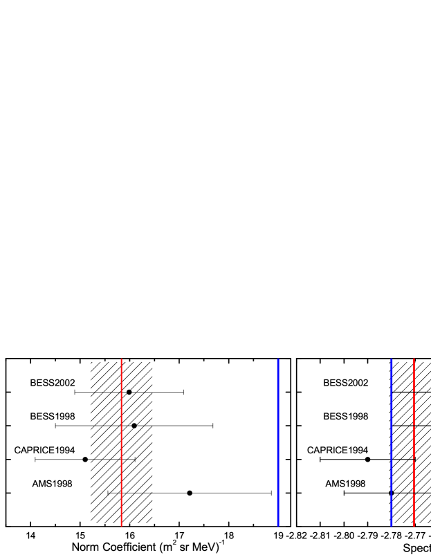
Figure 1: Fit (red line) of high energy proton spectrum measured by several experiments (black dots) and comparison with Burger & Potgieter[13]​ LIS (blue line). The spectral index is consistent with data, but the normalization constant is too large.

3.2 Latitudinal Gradient

Observations made by the Ulysses spacecraft in the inner heliosphere have shown that the latitudinal dependence of CR protons is significantly less than predicted by classical drift models[25]​. Our model, due to the modification of the $K_{\perp\theta}$[14]​ parameter in the polar regions can reproduce the gradient observed by Ulysses (see Fig. 3 in Heber et al.[25]​) between the poles and the ecliptic plane. We find, for the period of AMS-01 data taking (June 1998), a difference of $\sim$ 16 % between the ecliptic plane and a colatitude of $\sim 30^{\circ}$ from the poles. In Figure 2 a simulation of the proton differential intensity on the ecliptic plane is compared with the one at 30 deg from the poles (left panel). The latitudinal gradient of the integral intensity is shown in the right panel of Figure 2.

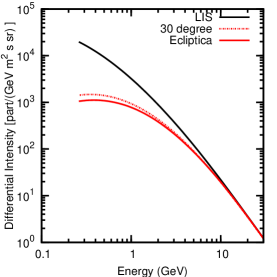
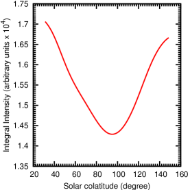
Figure 2: Left panel: simulation of the proton differential intensity on the ecliptic plane is compared with the same quantity at 30 deg from the poles. Right panel: the latitudinal gradient, i.e. the integral intensity for $E\geq 200$ MeV vs the solar colatitude. Simulations have been done using solar parameters occurred in June 1998.

4 Results

4.1 Proton differential intensity

We performed the simulations using dynamic values of $K_{0}$, $\alpha$ and $V_{sw}$: we consider present time parameters in the inner shell of the heliosphere, but we use the values assumed by the parameters up to 14 months back in the past at the heliopause. Results are shown in Figure 3. Simulated differential intensity with dynamic values shows a very good agreement with measured data, within the quoted error bars. This happens in periods with low solar activity and A$>$0, in comparison with AMS-01[22]​, BESS-97[21]​ and BESS-99[21]​; in periods with high solar activity, in comparison with BESS-00[21]​; and in periods with a lower solar activity and A$<$0, in comparison with BESS-02[23]​ and BESS-04[24]​. This means that our description of the Heliosphere improves the understanding of the complex processes occurring inside the solar cavity.

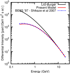
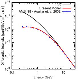
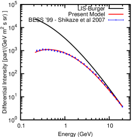
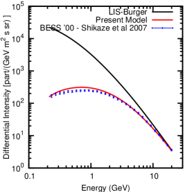
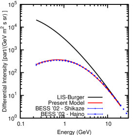
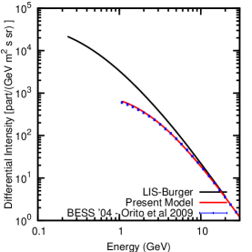
Figure 3: Comparison of simulated galactic proton differential intensity at 1 AU and experimental data: AMS-01[22]​ (1998) and BESS[21, 24]​ (1997, 1999, 2000, 2002, 2004).

4.2 AMS-02 Predictions

Our simulation code has been used to predict CR differential intensity for future measurements. The assumption is that diffusion parameter, tilt angle and solar wind speed show a near-regular and almost periodic trend. The periodicity occurs after two consecutive 11-years solar cycles. Using SIDAC (Solar Influences Data Analysis Center) data we selected periods with a nearly similar solar activity conditions and same solar field polarity of the simulation time: therefore approximately 22 years in advance. We concentrate our simulations on the AMS-02 mission, that will be installed on the ISS in February 2011, for a period approaching the solar maximum: January 2012. Results are shown in Fig. 4.

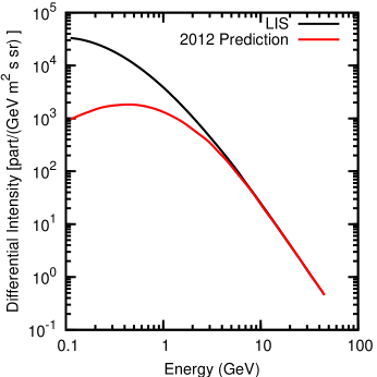
Figure 4: Prediction of modulated proton differential intensity as will be measured by AMS-02 experiment in January 2012.

The Sun is currently in an unpredicted long duration solar minimum, that forced scientists to review all their estimations for the next solar cycle, therefore this prediction could be object of revision in the next future. AMS-02 is expected to collect, in a few years of operation, more than $10^{10}$ protons with energy $\geq$ 1 GeV, and $\sim 10^{6}$ with energy $\geq$ 1 TeV.

5 Conclusions

We built a 2D stochastic Monte Carlo code for particles propagation inside the heliosphere. Our model takes into account drift effects and shows a good agreement with measured values, in periods with positive as well as with negative polarity. Proton spectra, as predicted by the model, are decreasing with increasing tilt angle and solar wind velocity. We use as input LIS the model published by Burger & Potgieter[13]​, corrected in order to fit the high energy measured intensity. Recent measurements have pointed out the needs to reach a high level of accuracy in the modulation of the differential intensity, in relation to the charge sign of the particles and the solar field polarity[26]​. This aspect will be even more crucial in the next generation of experiments.

References

- [1] P. Bobik, M. Gervasi, D. Grandi, P.G. Rancoita, and I.G. Usoskin, Proceedings of ICSC, 2003, ESA SP-533 (2003).
- [2] P. Bobik, et al., Proc. of the 11th ICATPP, Como 5–9/10/2009; Astroparticle, Particle, Space Physics, Detectors and Medical Physics Applications, 5, 210 (2010); World Scientific, Singapore, ISBN-13 978-981-4307-51-2.
- [3] G. Boella, M. Gervasi, S. Mariani, P.G. Rancoita, and I.G. Usoskin, J. Geophys. Res., 106, A12, 29355 (2001).
- [4] P. Bobik, G. Boella, M.J. Boschini, M. Gervasi, D. Grandi, K. Kudela, S. Pensotti, and P.G. Rancoita J. Geophys. Res., 111, A05205 (2006).
- [5] M.S. Potgieter, et al., Astroph. J., 403, 760 (1993).
- [6] L.A. Fisk, J. Geophys. Res., 81, 4646 (1976).
- [7] P. Bobik, et al., Proc. of the 11th ICATPP, Como 5–9/10/2009; Astroparticle, Particle, Space Physics, Detectors and Medical Physics Applications, 5, 760 (2010); World Scientific, Singapore, ISBN-13 978-981-4307-51-2.
- [8] C.W. Gardiner, Handbook of Stochastic Methods, Springer Verlag, Berlin (1989).
- [9] K. Alanko-Huotari, I.G. Usoskin, K. Mursula, and G.A. Kovaltsov, J. Geophys. Res., 112, A8, CiteID A08101, (2007).
- [10] P. Bobik, et al., “2D Stochastic Montecarlo to evaluate the modulation of GCR for positive and negative periods”, Proc. 21th ECRS 2008 (Košice, Slovakia) (2009).
- [11] P. Bobik, M. Boschini, M. Gervasi, D. Grandi, K. Kudela and P.G. Rancoita “Heliosphere modulation of Primary Comsic Rays for the AMS-02 mission”, Proceedings of the 31st ICRC, Lodz, Polonia, 2009.
- [12] M.S. Potgieter, and J.A. Le Roux, Astroph. J., 423, 817 (1994).
- [13] R.A. Burger, and M.S. Potgieter, Astroph. J., 339, 501 (1989).
-
[14]
P. Bobik, et al., 2011, Proton and antiproton modulation in the heliosphere for different solar conditions and
AMS-02 measurements prediction, Proc. of the ICATPP Conference on Cosmic Rays for Particle and Astroparticle Physics, October 7–8 2010, Villa Olmo, Como, Italy, Giani, S., Leroy, C. and Rancoita, P.G., Editors, World Scientific, Singapore, ISBN 978-981-4329-02-6; arXiv:1012.3086v3 [astro-ph.EP], available at the web site:
http://arxiv.org/abs/1012.3086 - [15] M.S. Potgieter, et al., Adv. Space Res., 19, No. 6, 917 (1997).
- [16] R.A. Burger, and M. Hitge, American Geophysical Union SH71A-04, Fall Meeting 2002.
- [17] J.R. Jokipii, and J. Kóta, Geophys. Res. Lett., 16, 1 (1989).
- [18] J.P.L. Reinecke, C.D. Steenberg, H. Moraal, F.B. McDonald, Adv. Space Res., 19, No. 6, 901 (1997).
- [19] M. Hatting, and R.A. Burger, Adv. Space Res. 16, No. 9, 213 (1995).
- [20] G.M. Boezio, et al., Astrophys. J., 518, 457 (1999).
- [21] Y. Shikaze, et al., Astropart. Phys., 28, 154 (2007).
- [22] J. Alcaraz, et al., Physics Lett. B, 490, 27 (2000).
- [23] S. Haino, et al., Physics Lett. B, 594, 35 (2004).
- [24] K.C. Kim, et al., Proc. 30th ICRC 2007 (Mexico City, Mexico), 2, 71 (2009).
- [25] B. Heber, et al., J. Geophys. Res., 103, A3, 4809 (1998).
- [26] G. Boella, M. Gervasi, M.C.C. Potenza, P.G. Rancoita and I.G. Usoskin, Astropart. Phys., 9, 261 (1998).