Kinetic analysis of a chiral granular motor

Abstract

We study the properties of a heterogeneous, chiral granular rotor that is capable of performing useful work when immersed in a bath of thermalized particles. The dynamics can be obtained in general from a numerical solution of the Boltzmann-Lorentz equation. We show that a mechanical approach gives the exact mean angular velocity in the limit of an infinitely massive rotor. We examine the dependence of the mean angular velocity on the coefficients of restitution of the two materials composing the motor. We compute the power and efficiency and compare with numerical simulations. We also perform a realistic numerical simulation of a granular rotor which shows that the presence of non uniformity of the bath density within the region where the motor rotates, and that the ratchet effect is slightly weakened, but qualitatively sustained. Finally we discuss the results in connection with recent experiments.

1 Introduction

Much is known about the properties of Brownian ratchets and their applications in physics and biology. Smoluchowski’s [1] original proposal consisted of a device with four vanes connected to a ratchet and pawl. When immersed in a thermalized bath of particles the device can apparently rectify the thermal fluctuations to produce useful work. Feynmann[2], however, demonstrated that this is not possible if the entire system is at thermal equilibrium. The device only performs work if the vanes and the ratchet and pawl are maintained at different temperatures, $T_{1}$ and $T_{2}$, respectively with $T_{1}>T_{2}$. It is now understood that the general requirements for a functioning motor are the absence of both time and spatial symmetry. The former occurs if there is a breakdown of detailed balance and the latter may be due to the intrinsic asymmetry of the object itself or to an external force [3, 4, 5].

In the last few years, several proposals for granular motors have appeared. The dissipative nature of inelastic collisions leads to an automatic breakdown of time reversal symmetry and the spatial asymmetry can be created in various ways. In 2007 Cleuren and Van den Broeck [6] and independently, Costantini, Marconi and Puglisi [7, 8] proposed the same model granular motor, viz. an isosceles triangle composed of a homogeneous inelastic material constrained to move along a line. When immersed in a bath of thermalized particles, the undirected fluctuations of the bath particles induce a directed motion of the triangle. The drift velocity is proportional to $(1-\alpha)\sqrt{m/M}\sqrt{\frac{kT}{M}}$ where $\alpha$ is the coefficient of restitution characterizing the collision between the tagged particle (of mass $M$) and the bath particles (of mass $m$). This result shows that the phenomenon is specific to granular particles, because the drift velocity vanishes when $\alpha=1$. Also, because the granular temperatures of the tagged particle and the bath particles are comparable, whatever the mass ratio, $<(V-<V>)^{2}>$ decreases as $m/M$ (for a given bath temperature), and this results in a signal-to-noise ratio that vanishes for large values of $\sqrt{m/M}$.

Cleuren and Eichhorn [9] later proposed an alternative model consisting of a homogeneous rotor that is constrained to rotate about an off-center axis. If the material composing the rotor is inelastic, a net rotation is obtained and it displays the same dependence on $\alpha$ and $m/M$ as the triangle, which complicates the experimental observation of this phenomena.

Fortunately, this difficulty can be overcome by using a heterogeneous device constructed from two different materials with different coefficients of restitution. This leads to a strong ratchet effect [10]. Costantini et al. [11] proposed possibly the simplest model of a granular motor of this type, the asymmetric piston composed of two materials with different inelasticities. Starting from the Boltzmann equation, they proposed a phenomenological approach based on the evolution of the first three moments of the velocity distribution. Although their theory is in good agreement with numerical simulation results in some cases, it breaks down in the limit of large piston mass.

Recently, Eshuis et al. [12] succeeded in constructing a macroscopic rotational ratchet consisting of four vanes that rotates in a granular gas. They performed two kinds of experiments: in the first, the vanes were symmetric and no net angular velocity was observed. In the second, asymmetry was induced by coating each side of the vanes differently. For sufficiently large granular temperatures of the bath particles, a net rotation is observed. We will discuss the implications of this experiment in the concluding section.

In a recent article [13] we presented a mechanical approach that gives the average force acting on a heterogeneous particle moving at a given velocity. The mechanical approach is consistent with the Boltzmann equation and in the Brownian limit, $m/M\rightarrow 0$, it leads directly to an exact expression for steady state drift velocity.

From both technological and fundamental perspectives, the power and efficiency of thermal engines are of major interest. Indeed, Carnot’s analysis of an idealized heat engine is a landmark event in the history of thermodynamics. His famous result for the efficiency depends only the temperatures of the heat reservoirs, but applies strictly to a reversible - and hence quasi-static - process. The efficiency at non-zero power was first considered by Curzon and Ahlborn[14] and later generalized by van den Broeck [15]. The efficiency of Brownian motors has also been discussed [16, 17], but there has been little discussion of the power and efficiency of granular motors [13]. Such considerations are, nevertheless, of great importance for the practical realization of these devices.

It is the purpose of this article to apply the approach first proposed in [13] to the chiral rotor. We also investigate the effect of bath inhomogeneities with a realistic numerical experiment. Finally, we show that the mechanical approach provides an explanation for the presence of a threshold for the rotation of the vanes in the experiment of Eshuis et al. [12].

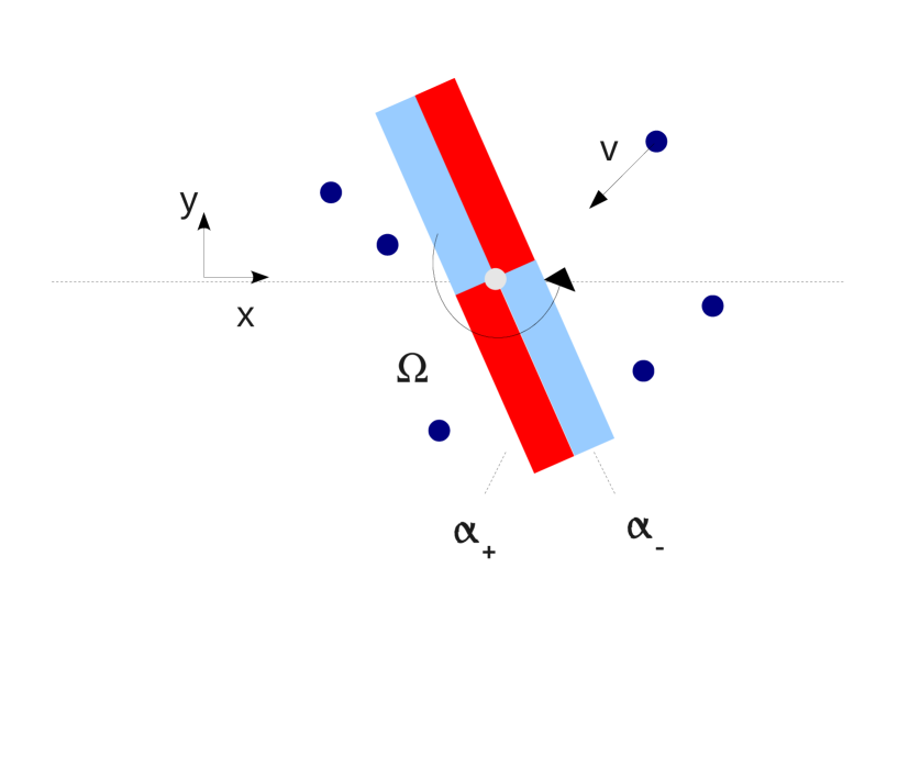
Figure 1: The chiral rotor is constructed from two different materials with coefficients of restitution $\alpha_{+}$ (red) and $\alpha_{-}$ (blue). When immersed in a bath of thermalized particles, it acquires a net rotation around its axis.

2 Model

The chiral rotor is composed of two materials with coefficients of restitution $\alpha_{+}$ and $\alpha_{-}$: See figure 1. Collisions of the bath particles with the former result in a positive torque (anticlockwise sense), while collisions with the material with $\alpha_{-}$ result in a negative torque. The device is immersed in a two-dimensional granular gas composed of structureless particles at a density $\rho$ each of mass $m$.

An important assumption of the model is that collisions between the motor and the bath particles do not modify the velocity distribution of the latter. This neglect of recollisions is consistent with the foundations of Boltzmann’s kinetic theory. We let $v_{\perp}$ and $v_{\parallel}$ denote the components of the gas particle’s velocity perpendicular and parallel to the surface of the motor, respectively. The granular temperature of the bath is defined as $T_{B}=m<v_{\perp}^{2}>=m<v_{\parallel}^{2}>$. Since $v_{\parallel}$ is irrelevant in the Boltzmann-Lorentz description of the rotor[18], for sake of simplicity we denote $v_{\perp}$ by $v$ in the rest of the section.

Wherever possible, we will give results for an arbitrary bath particle velocity distribution, $\phi(v)=\int dv_{\parallel}\phi({\bf v})$. Sometimes, though, it will be necessary to assume a particular form and in this case we will use a Maxwell-Boltzmann or Gaussian distribution:

$$\phi_{MB}(v)=\frac{1}{\sqrt{2\pi}v_{th}}\exp\left(-\frac{v^{2}}{2v_{th}^{2}}\right),$$ (1)

where $v_{th}=\sqrt{T_{B}/m}$. While granular gases often have non-Maxwellian velocity distributions, it is possible to devise experimental situations where the Gaussian distribution is observed [19, 20].

The collision equations are

$$\left(\begin{array}[]{c}\Omega^{\prime}\\ v^{\prime}\\ \end{array}\right)=\left(\begin{array}[]{c}\Omega\\ v\\ \end{array}\right)+\frac{1+\alpha}{I+mx^{2}}(v-\Omega x)\left(\begin{array}[]{c}mx\\ -I\\ \end{array}\right)$$ (8)

where $\Omega$ is the angular velocity, $I$ is the moment of inertia and $-L/2\leq x\leq L/2$ is the algebraic distance of impact from the center (for simplicity, we neglect collisions between bath particles and the caps of the rotor). The granular temperature of the rotor is given by $T_{g}=I<(\Omega-<\Omega>)^{2}>$. Because the mass of any section of thickness $\Delta x$ perpendicular to the long axis of the rotor is constant, the moment of inertia is the same as for a homogeneous rotor, $I=ML^{2}/12$, where $M$ is the total mass. The energy loss on collision is

$$\Delta E=-\frac{mI(1-\alpha^{2})(v-\Omega x)^{2}}{2(I+mx^{2})}$$ (9)

The reconstituting velocities are

$$\left(\begin{array}[]{c}\Omega^{**}\\ v^{**}\\ \end{array}\right)=\left(\begin{array}[]{c}\Omega\\ v\\ \end{array}\right)+\frac{1+\alpha^{-1}}{I+mx^{2}}(v-\Omega x)\left(\begin{array}[]{c}mx\\ -I\\ \end{array}\right)$$ (16)

3 Boltzmann-Lorentz Equation

The time dependent Boltzmann-Lorentz equation for the chiral rotor is

$$\frac{\partial}{\partial t}f(\Omega;t) =\rho\int_{-L/2}^{L/2}dx\,\int_{-\infty}^{\infty}dv\;|v-x\Omega|\left[\theta(v-x\Omega)\frac{f(\Omega^{**};t)}{\alpha_{+}^{2}}\phi(v^{**})+\theta(x\Omega-v)\frac{f(\Omega^{**};t)}{\alpha_{-}^{2}}\phi(v^{**})\right]$$ (17)

$$-\rho f(\Omega;t)\int_{-L/2}^{L/2}dx\,\int_{-\infty}^{\infty}dv\;|v-x\Omega|\phi(v)$$

where $\theta(x)$ is the Heaviside function. By introducing the variable $y=(v-\Omega x)/\alpha_{+}$, $y=(\Omega x-v)/\alpha_{-}$ and exploiting the symmetry of the object we can write the equation in the more explicit and useful form:

$$\frac{1}{2\rho}\frac{\partial}{\partial t}f(\Omega;t) =\int_{0}^{L/2}dx\,\int_{0}^{\infty}dy\;yf\left(\Omega-\frac{1+\alpha_{+}}{I+mx^{2}}mxy\right)\phi\left(\Omega x+\frac{I-\alpha_{+}mx^{2}}{I+mx^{2}}y\right)$$ (18)

$$+\int_{0}^{L/2}dx\,\int_{0}^{\infty}dy\;yf\left(\Omega+\frac{1+\alpha_{-}}{I+mx^{2}}mxy\right)\phi\left(\Omega x-\frac{I-\alpha_{-}mx^{2}}{I+mx^{2}}y\right)$$

$$-f(\Omega)\int_{0}^{L/2}dx\,\int_{0}^{\infty}dy\;y(\phi(\Omega x+y)+\phi(\Omega x-y))$$

When the bath distribution is Gaussian, equation 1, one can confirm that for a rotor with $\alpha_{+}=\alpha_{-}=1$, the solution in the steady state is given by $f(\Omega)=\sqrt{I/2\pi T_{B}}\exp(-I\Omega^{2}/2T_{B})$.

3.1 Numerical solution

The Direct Simulation Monte Carlo (DSMC) method [21] is often used to obtain numerical solutions of the Boltzmann equation and has been applied to granular systems [22]. An alternative is the Gillespie method [23]. In this application, the linear nature of the Boltzmann-Lorentz equation makes it well suited to solution by iteration. To achieve this, we rewrite the equation in the following form:

$$f^{(n+1)}(\Omega) =\frac{1}{\nu(\Omega)}\left[\int_{0}^{L/2}dx\,\int_{0}^{\infty}dy\;yf^{(n)}\left(\Omega-\frac{1+\alpha_{+}}{I+mx^{2}}mxy\right)\phi\left(\Omega x+\frac{I-\alpha_{+}mx^{2}}{I+mx^{2}}y\right)\right.$$ (19)

$$\left.+\int_{0}^{L/2}dx\,\int_{0}^{\infty}dy\;yf^{(n)}\left(\Omega+\frac{1+\alpha_{-}}{I+mx^{2}}mxy\right)\phi\left(\Omega x-\frac{I-\alpha_{-}mx^{2}}{I+mx^{2}}y\right)\right]$$

where $f^{(n)}$ denotes the $n$th iteration and

$$\nu(\Omega)=\int_{0}^{L/2}dx\,\int_{0}^{\infty}dy\;y(\phi(\Omega x+y)+\phi(\Omega x-y))$$ (20)

so that $2\rho\nu(\Omega)$ is the collision rate when the motor rotates with angular velocity $\Omega$. We take as the initial guess, $f^{(0)}$, either a Gaussian distribution or the previous converged solution for different parameters. The error is defined as

$$\epsilon=\int_{-\infty}^{\infty}[f^{(n+1)}(\Omega)-f^{(n)}(\Omega)]^{2}\,d\Omega$$ (21)

In the results reported here we took the solution as converged when $\epsilon<10^{-15}$.

We show some results in figure 2. As the rotor becomes heavier, the distribution becomes more Gaussian with the maximum at the drift velocity $\Omega^{*}$. Conversely a light rotor has a markedly non-Gaussian distribution that becomes more and more skewed with decreasing mass. For a sufficiently light rotor, the most probable angular velocity is opposite in sign to the mean value. This is similar to the behavior observed for the asymmetric piston [7].

The increasingly non-Gaussian behavior can be quantified by examining the skewness and kurtosis, $\kappa$, of the distribution: See figure 3 (for convenience the excess kurtois, defined as $\kappa-3$, is shown). While the excess kurtosis is nearly zero beyond $I/mL^{2}=1$, there is some residual skewness for large rotor masses. We also note the the granular temperature of the rotor varies little beyond $I/mL^{2}=1$.

3.2 Kramers-Moyal expansion

Henceforth we focus on the Brownian limit as it is more interesting for the experimental application. As with the piston[13] we can perform a series expansion of Boltzmann equation by introducing the small parameter $\epsilon=\sqrt{\frac{mL^{2}}{I}}$, the variable $z=(\Omega-\Omega^{*})/\epsilon$ where $\Omega^{*}$ is the drift velocity in the Brownian limit, and a rescaled velocity distribution $F(z)$. At first order we obtain

$$\int_{0}^{\infty}dy\;\int_{0}^{L/2}dx\;xy^{2}((1+\alpha_{+})\phi(x\Omega^{*}+y)-(1+\alpha_{-})\phi(x\Omega^{*}-y))=0,$$ (22)

which can be solved numerically to obtain $\Omega^{*}$. At second order we obtain a Fokker-Planck equation for the rotor angular velocity distribution that gives, in the original variables

$$f(\Omega)\propto e^{-I(\Omega-\Omega^{*})^{2}/2T_{g}}.$$ (23)

where $T_{g}/m$ is given by

$$\frac{T_{g}}{m}=\frac{\int_{0}^{L/2}dx\;\int_{0}^{\infty}dy\,x^{2}\,y^{3}((1+\alpha_{-})^{2}\phi(\Omega^{*}x\!-\!y)\!+\!(1+\alpha_{+})^{2}\phi(\Omega^{*}x\!+\!y))}{4\int_{0}^{L/2}dx\;\int_{0}^{\infty}dy\,x^{2}\,y((1+\alpha_{-})\phi(\Omega^{*}x\!-\!y)+(1+\alpha_{+})\phi(\Omega^{*}x\!+\!y))}$$ (24)

For a rotor with $\alpha_{+}=1,\alpha_{-}=0$ in a Gaussian bath, equation (1), we find $T_{g}/T_{B}=0.72960$ which is close to the value for the corresponding asymmetric piston ($T_{g}/T_{B}=0.73460$).

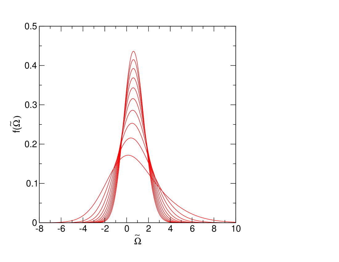
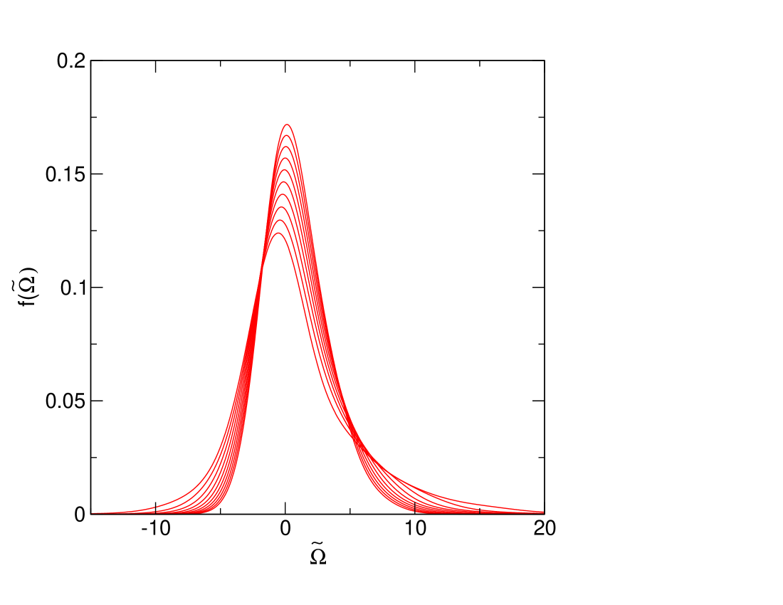
Figure 2: Angular velocity distributions for a chiral rotor with $\alpha_{-}=0$, $\alpha_{+}=1$ obtained by iteration of the Boltzmann equation. Top: $1\leq I\leq 10$ in steps of 1; Bottom $0.1\leq I\leq 1.0$ in steps of 0.1

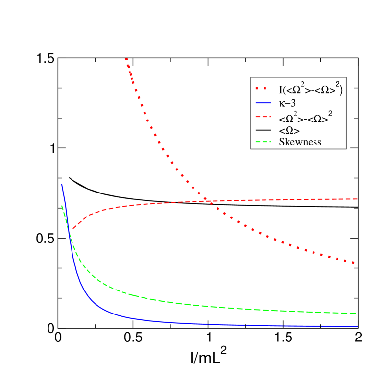
Figure 3: First moment (second from top, right hand side), second moment (third from bottom, right hand side), skewness (second from bottom, right hand side) and excess kurtosis (bottom curve) of the velocity distribution for $\alpha_{-}=0$, $\alpha_{+}=1$ as a function of $\mu$. The dashed line shows the granular temperature of the rotor.

.

4 Torque-based approach

The instantaneous impulse exerted on the rotor of angular velocity $\Omega$ by a collision with a bath particle of velocity $v$ on a face with $\alpha_{+}$ is

$$I_{-} =I\Omega^{\prime}-I\Omega$$ (25)

$$=-\frac{Imx}{I+mx^{2}}(I+\alpha_{-})(\Omega x-v),\;\;\;v<\Omega x$$

Similarly for a collision on a face with $\alpha_{-}$

$$I_{+}=\frac{Imx}{I+mx^{2}}(I+\alpha_{+})(v-\Omega x),\;\;\;\Omega x<v$$ (26)

Assuming that successive collisions between bath particles and the granular motor are uncorrelated, averaging on different collisions at a given $\Omega$ consists of integrating the impulse times the rate that the specified face collides with a particle moving with a velocity $v$: Evaluation of the torque requires an integral over $x$, in addition to the bath particle velocity distribution, i.e.

$$\Gamma_{-}(\Omega) =2\rho\int_{0}^{L/2}dx\;\int_{-\infty}^{\Omega x}dv\;I_{-}(\Omega,v)(\Omega x-v)\phi(v)$$ (27)

$$\Gamma_{+}(\Omega) =2\rho\int_{0}^{L/2}dx\;\int_{\Omega x}^{\infty}dv\;I_{+}(\Omega,v)(v-\Omega x)\phi(v)$$ (28)

We suppose that, in addition to the fluctuating force resulting from collisions with the bath particles, the rotor is subject to a constant external torque, $\Gamma_{\rm ext}$. The average of the net torque performed over all possible angular velocities of the rotor is equal to zero in the stationary state. Since the successive collisions are assumed uncorrelated, this condition can be expressed as,

$$<\Gamma_{\rm net}(\Omega)>=\int_{-\infty}^{\infty}d\Omega f(\Omega)\Gamma(\Omega)+\Gamma_{\rm ext}=0$$ (29)

where $\Gamma(\Omega)=\Gamma_{-}(\Omega)+\Gamma_{+}(\Omega)$. It is convenient to rewrite this as

$$<\Gamma_{\rm net}(\Omega)>=\Gamma(<\Omega>)+\Gamma_{f}+\Gamma_{\rm ext}=0$$ (30)

where $\Gamma(<\Omega>)$ is the mean torque when the rotor has constant angular velocity, $<\Omega>$ and $\Gamma_{f}$ is the mean torque resulting from the fluctuations of the angular velocity around the mean value, $<\Omega>$. Now by expanding $\Gamma(\Omega)$ about $\Omega^{*}$, where $\Gamma(\Omega^{*})=0$ we have that

$$\Gamma_{f} = <(\Omega-\Omega^{*})\Gamma^{\prime}(\Omega^{*})+\frac{1}{2}(\Omega-\Omega^{*})^{2}\Gamma^{\prime\prime}(\Omega^{*})+$$ (31)

$$+\frac{1}{6}(\Omega-\Omega^{*})^{3}\Gamma^{\prime\prime\prime}(\Omega^{*})+...>-\Gamma(<\Omega>)$$

So to lowest order the angular velocity is given by

$$<\Omega>=\Omega^{*}-\frac{\frac{1}{2}\Gamma^{\prime\prime}(\Omega^{*})<(\Omega-\Omega^{*})^{2}>+\Gamma_{\rm ext}}{\Gamma^{\prime}(\Omega^{*})}$$ (32)

Since $I<(\Omega-\Omega^{*})^{2}>\approx T_{g}$, we have that in the Brownian limit, $I\rightarrow\infty$,

$$<\Omega>=\Omega^{*}-\Gamma_{\rm ext}/\Gamma^{\prime}(\Omega^{*})+O(1/I)$$ (33)

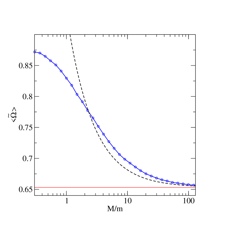
Figure 4: Dimensionless mean angular velocity $\tilde{\Omega}$ as a function of the mass ratio $M/m$ for $\alpha_{+}=1$ and $\alpha_{-}=0$. The joined circles show the simulation results, the solid horizontal line is the exact result in the Brownian limit (the solution of $\Gamma(\Omega)=0$ with $\Gamma(\Omega)$ given by equation (38)) and the dashed line shows the first order correction, equation (35).

Making the substitutions $y=\Omega x-v$ and $y=v-\Omega x$, we find the following expression for the total torque in the Brownian limit, $mL^{2}/I\rightarrow 0$:

$$\Gamma(\Omega)=2m\rho\int_{0}^{L/2}dx\int_{0}^{\infty}dy\;xy^{2}((1+\alpha_{+})\phi(x\Omega+y)-(1+\alpha_{-})\phi(x\Omega-y))$$ (34)

We obtain the mean angular velocity, $\Omega^{*}$, by setting the torque equal to zero: $\Gamma(\Omega^{*})=0$.

The result, as well as simulations for finite ratios are shown in figure 4. Note that, unlike the piston [13], we do not observe a maximum as the moment of inertia decreases.

We can also calculate corrections to the Brownian limit by using equation (32)

$$<\Omega>\simeq\Omega^{*}-\frac{1}{2}\frac{\Gamma^{\prime\prime}(\Omega^{*})}{\Gamma^{\prime}(\Omega^{*})}\frac{T_{g}}{I}$$ (35)

$T_{g}$, $\Gamma^{\prime}(\Omega^{*})$ and $\Gamma^{\prime\prime}(\Omega^{*})$ are functions of $\alpha_{+}$ and $\alpha_{-}$. Figure 4 shows that, for $\alpha_{-}=0,\alpha_{+}=1$, the first order correction provides a reasonably accurate description for $M/m>5$, but for smaller values it diverges in contrast to the exact result that approaches a finite value.

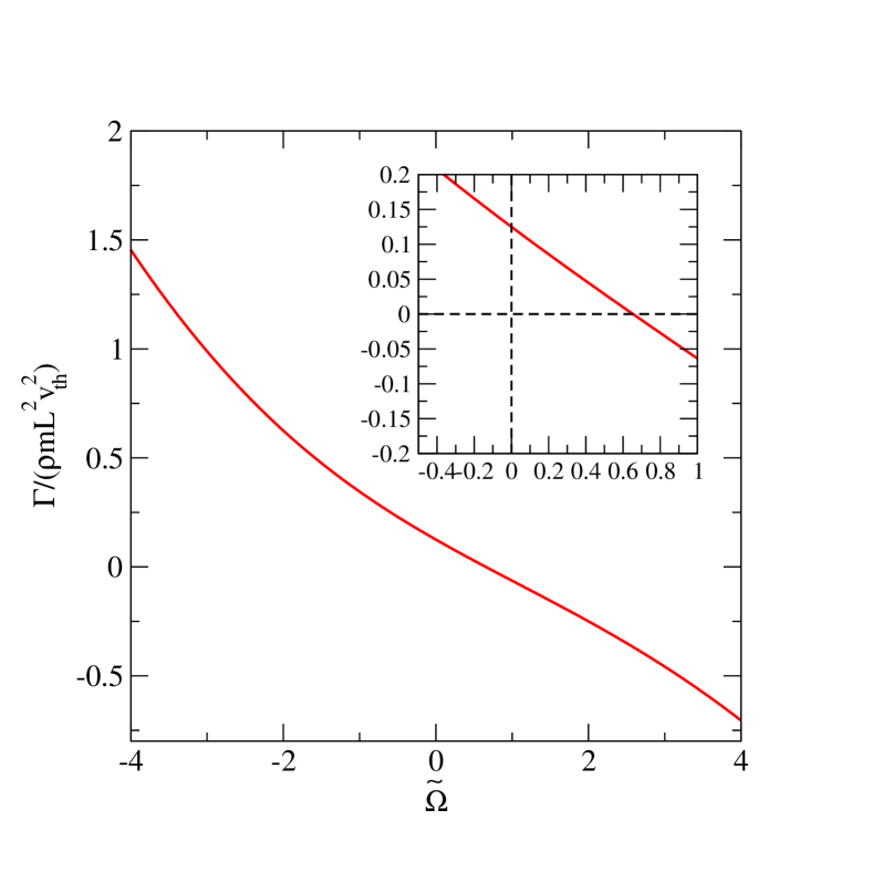
Figure 5: Dimensionless torque as a function of the mean angular velocity $\tilde{\Omega}$ for $\alpha_{+}=1$ and $\alpha_{-}=0$. The torque is positive for $\tilde{\Omega}=0$ and vanishes for a positive value of $\tilde{\Omega}$, which corresponds to the solution of $\Gamma(\Omega)=0$ with $\Gamma(\Omega)$ given by equation (38). At large angular velocity, the torque is opposite in sign to the angular velocity.

For an arbitrary symmetric bath distribution, the torque on a stationary rotor in the Brownian limit is

$$\Gamma(0)=\frac{1}{8}m\rho L^{2}(\alpha_{+}-\alpha_{-})<v^{2}>$$ (36)

In an experimental situation, this must exceed the solid friction for the motor to function.

For small variations of the angular velocity, the torque exerced by the particle bath is proportional to the deviations from the steady state $\Gamma(\Omega)=(\Omega^{*}-\Omega)\Gamma^{\prime}(\Omega^{*})$ where $\Gamma^{\prime}(\Omega^{*})$ is always a nonzero negative constant.

At large angular velocities, one obtains that

$$\Gamma(\Omega)\simeq\mp\frac{m(1+\alpha_{\mp})\rho L^{4}}{32}\Omega^{2},\;\;\Omega\rightarrow\pm\infty$$ (37)

The damping is quadratic at large values of the velocity (the piston has a similar behavior).

For a Gaussian distribution in the Brownian limit, we can obtain an analytical expression for the torque:

$$\frac{\Gamma}{m\rho L^{2}v_{th}^{2}} =\frac{\alpha_{+}-\alpha_{-}}{64}(\tilde{\Omega}^{2}+8)-(2+\alpha_{+}+\alpha_{-})$$ (38)

$$\left[\frac{1}{64}(\tilde{\Omega}^{2}+8-\frac{16}{\tilde{\Omega}^{2}})erf(\frac{\tilde{\Omega}}{2\sqrt{2}})+\frac{1}{32}\sqrt{\frac{2}{\pi}}(\tilde{\Omega}+\frac{4}{\tilde{\Omega}})\exp(-\tilde{\Omega}^{2}/8)\right]$$

where $\tilde{\Omega}=\Omega L/v_{th}$ (see figure 5). Expanding in powers of $\tilde{\Omega}$ to obtain

$$\frac{\Gamma}{m\rho L^{2}v_{th}^{2}}=\frac{1}{8}(\alpha_{+}-\alpha_{-})-\frac{1}{12}\sqrt{\frac{2}{\pi}}(2+\alpha_{+}+\alpha_{-})\tilde{\Omega}+O(\tilde{\Omega}^{3})$$ (39)

from which we can obtain an analytical estimate for the angular velocity in the steady state

$$\tilde{\Omega}^{*}=\frac{3}{2}\sqrt{\frac{\pi}{2}}\frac{\alpha_{+}-\alpha_{-}}{2+\alpha_{+}+\alpha_{-}}$$ (40)

We note that this differs from the result for the asymmetric piston [13] by a constant factor. This result also shows that, for given coefficients of restitution and bath properties, the rotational velocity is inversely proportional to the length of the rotor.

4.1 Dependence of the mean angular velocity on the coefficients of restitution

We examine the mean angular velocity in the Brownian limit as a function of the coefficients of restitution. It is easy to show starting from $\Gamma(\Omega^{*})=0$ with $\Gamma(\Omega)$ given by equation (34) that $\Omega^{*}(\alpha_{+}=x,\alpha_{-}=y)=-\Omega^{*}(\alpha_{+}=y,\alpha_{-}=x)$, regardless of the bath distribution. Of course this result is expected from simple symmetry considerations. In figure 6 we show $\Omega^{*}(\alpha_{+}=x,\alpha_{-}=0)$ and $\Omega^{*}(\alpha_{+}=1,\alpha_{-}=x)$ as a function of $x$ in the case of a Gaussian bath distribution. The former increases as $x$ increases, while the latter decreases. They are equal for a particular value of $x$ and from equation (38) we may show that this occurs for $x=\sqrt{2}-1$. These results illustrate that the mean angular velocity is not simply proportional to the difference in coefficients of restitution. Specifically, we can construct two rotors. The first is composed of an elastic material ($\alpha_{+}=1$), and another material with a coefficient of restitution of $x=\sqrt{2}-1$ or a difference of $2-\sqrt{2}=0.5858$. This has the same drift velocity as a second rotor composed of a completely inelastic material, ($\alpha_{-}=0$), and one with $\alpha_{-}=x$ or a difference of 0.4142.

These functions are very nearly symmetric i.e., to a good approximation they satisfy

$$\Omega^{*}(\alpha_{+}=x,\alpha_{-}=0)+\Omega^{*}(\alpha_{+}=1,\alpha_{-}=x)=\Omega^{*}(1,0)$$ (41)

Figure 6 also shows that the exact solutions are well-approximated by the second order estimate equation (40).

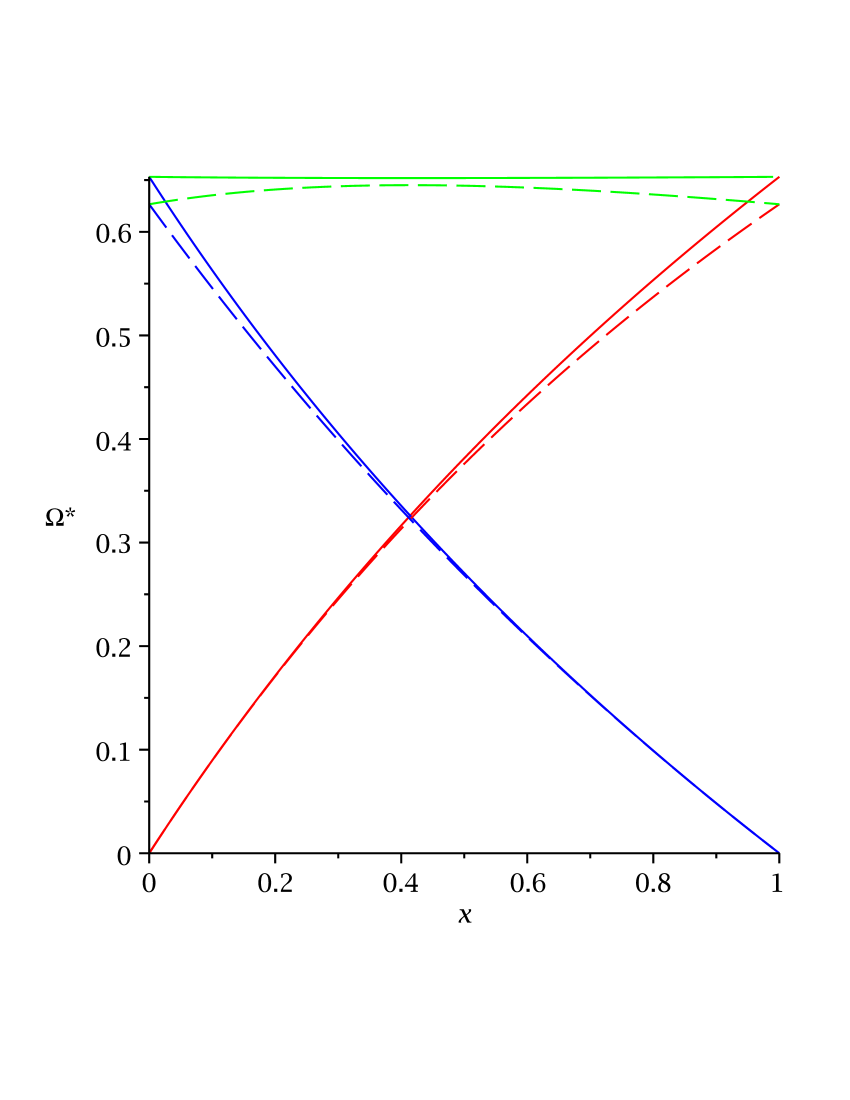
Figure 6: $\Omega^{*}(\alpha_{+}=x,\alpha_{-}=0)$ and $\Omega^{*}(\alpha_{+}=1,\alpha_{-}=x)$ and their sum as a function of $x$. The solid lines show the solution of $\Gamma(\Omega^{*})=0$ with $\Gamma(\Omega)$ given by equation (38) and the dashed lines show the approximate solution, equation (40).

4.2 Power and efficiency

A defining characteristic of granular motors is their ability to extract energy from the bath in the form of mechanical work. We now proceed to the calculation of the mechanical work, as well as the dissipated power due to the inelastic collisions between the granular motor and the bath particles. The ratio of these two quantities defines the efficiency of the motor.

If the external torque in equation (29) is non-zero, work is being done by, or on, the rotor. The power is given by

$$\dot{W}=\Gamma_{\rm ext}<\Omega>$$ (42)

In the Brownian limit we can estimate the average drift velocity using equation (33). Alternatively, we can take $<\Omega>$ as the independent variable:

$$\dot{W}=\Gamma(<\Omega>)<\Omega>$$ (43)

with $\Gamma(\Omega)$ given by equation (34). Of course, this approach is only valid in the Brownian limit. In general $\dot{W}(\Omega)$ has a parabolic form and is maximum for $0<\Omega<\Omega^{*}$. When the angular velocity is greater than $\Omega^{*}$ the power is negative, implying that it is necessary to drive the rotor externally in order to maintain the motion.

At second order

$$\frac{\dot{W}}{m\rho Lv_{th}^{3}}=\frac{1}{8}(\alpha_{+}-\alpha_{-})\tilde{\Omega}-\frac{1}{12}(2+\alpha_{+}+\alpha_{-})\sqrt{\frac{2}{\pi}}\tilde{\Omega}^{2}$$ (44)

Figure 7 shows that this provides a good approximation. The maximum power occurs at $\Omega_{mp}=\Omega^{*}/2$ and is given by

$$\frac{\dot{W}_{\rm max}}{m\rho Lv_{th}^{3}}=\frac{3\sqrt{2\pi}}{128}\frac{(\alpha_{+}-\alpha_{-})^{2}}{2+\alpha_{+}+\alpha_{-}}$$ (45)

From equation (9), we find that the rate of energy dissipation resulting from collisions between the bath particles and the rotor is

$$\dot{E}_{tot}(\Omega)=-m\rho\int_{0}^{L/2}dx\int_{0}^{\infty}dy\;y^{3}[(1-\alpha_{-}^{2})\phi(\Omega x-y)+(1-\alpha_{+}^{2})\phi(\Omega x+y)]$$ (46)

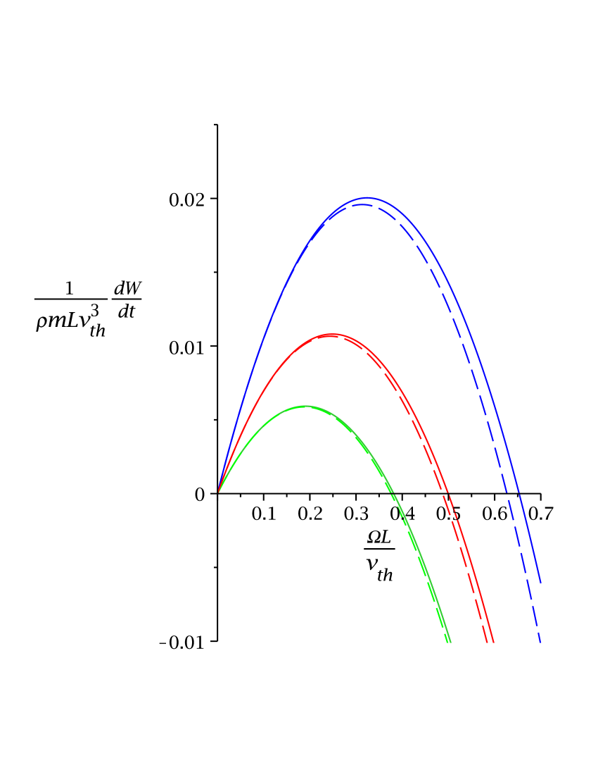
Figure 7: Power as a function of the rotor angular velocity for a system with $\alpha_{-}=0$ in the Brownian limit. The solid and dashed lines show the exact (equation (38) in equation (43)) and approximate (equation (44)) values, respectively. $\alpha_{+}=1,0.7,0.5$ in order of decreasing amplitude

The efficiency, or the fraction of the dissipated energy that is converted into work, is:

$$\eta(\alpha_{+},\alpha_{-},\Omega)=\frac{\dot{W}}{|\dot{E}_{tot}|}$$ (47)

For an arbitrary bath distribution in the Brownian limit we find that

$$\frac{\eta(\Omega,\alpha_{+},\alpha_{-})}{2\Omega}=\frac{\int_{0}^{L/2}dx\int_{0}^{\infty}dy\;xy^{2}((1+\alpha_{+})\phi(x\Omega+y)-(1+\alpha_{-})\phi(x\Omega-y))}{\int_{0}^{L/2}dx\int_{0}^{\infty}dy\;y^{3}((1-\alpha_{+}^{2})\phi(x\Omega+y)+(1-\alpha_{-}^{2})\phi(x\Omega-y))}$$ (48)

For a Gaussian bath distribution this has a maximum value of 4.3335% for $\alpha_{+}=1,\alpha_{-}=0,\tilde{\Omega}=0.29864$. Figure 8 shows the efficiency as a function of the dimensionless mean angular velocity obtained by simulation for several mass ratios, $M/m$ as well as the theoretical result in the Brownian limit, equation (48).

This mechanical analysis indicates that heterogeneous granular particles are able to produce significant noise rectification. Provided that the solid friction about the axis is not too large, the chiral rotor should be a good candidate for an experimental realization of a Brownian granular motor.

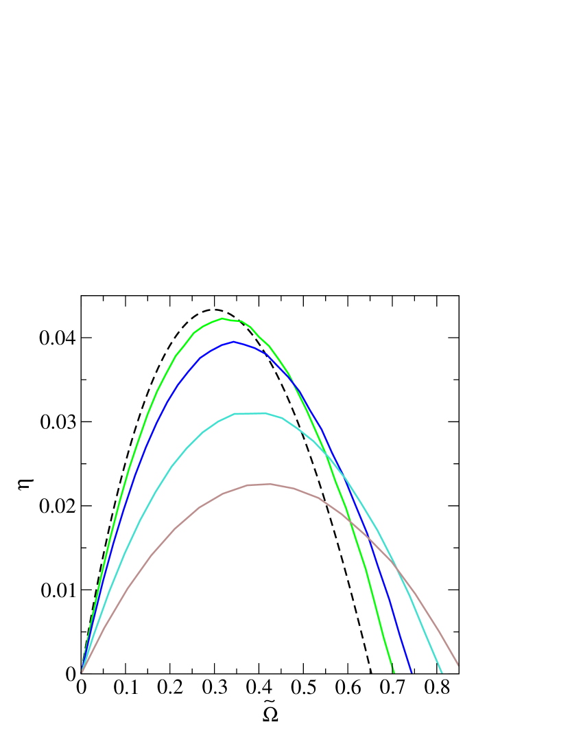
Figure 8: The efficiency as a function of the dimensionless mean drift angular velocity for a system with $\alpha_{-}=0,\alpha_{+}=1$. The solid curves show simulation results for $M/m=1,2,5,10$ (bottom to top), while the dashed line shows the theoretical prediction in the Brownian limit. The bath particle velocity distribution is given by equation (1).

5 Generalization to an n-vaned rotor

If one retains the assumption that the bath remains homogeneous and is not influenced by the presence of the rotor, it is easy to generalize the above analysis to a rotor composed of $n$ vanes. In the Boltzmann-Lorentz equation (18), the factor of $1/2\rho$ on the left hand side is replaced by $1/n\rho$. In the steady state the entire left hand side is equal to zero, so the steady state angular velocity is unchanged. In the expression for the torque, the factor of $2$ in equation (34) is replaced by $n$. But since this factor does not affect the solution of $\Gamma(\Omega^{*})=0$, the number of vanes has no effect on $\Omega^{*}$. We note, however, that the assumption of bath homogeneity certainly deteriorates as the number of vanes increases.

6 A numerical experiment

The analysis presented in the preceeding sections assumes that the bath is perfectly homogeneous. To investigate effect of relaxing this assumption, we now consider a realistic simulation of a quasi two-dimensional rotor. Burdeau et al.[24] developed a model that accurately reproduces an experimental study of a vibrated bilayer. The first layer consists of densely packed heavy granular particles while the second layer is composed of light particles with an intermediate coverage. Both experimentally and in the simulation, one observes a horizontal velocity distribution function of the light particles that is very close to a Gaussian [24].

To this vibrating bilayer system, we have added here a three dimensional spherocylinder constrained to rotate around a vertical axis: See figure 9. The spherocylinder cannot move horizontally or vertically: the rotation around the Oz axis is the sole degree of freedom. Figure 10 is a projection of the spherocylinder together with the geometrical parameters.

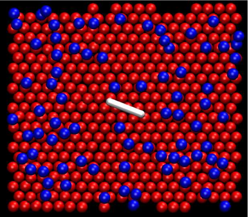
Figure 9: Top view of the simulation cell of size $20\times 20$ sphere diameters: The spherocylinder has a radius $R=2/3r$ ($r$ is the radius of the spheres) and a total length $L+2R$ where $L=11R$.

Figure 10: Geometry of the spherocylinder and a sphere during a collision

The simulation uses a Discrete Element Method where collisions between particles, collisions between spherocylinder and particles as well as collisions with the vibrating plate are all inelastic. In addition, the particles are subject to a constant acceleration due to the (vertical) gravitational field. The visco-elastic forces are modeled by the spring-dashpot model [25].

The systems consists of $N_{1}$ spheres placed in the first layer and $N_{2}$ spheres in the second layer. By choosing the system parameters as close as possible to the original experimental system[19], no mixing is observed between layers and the horizontal velocity distribution of the second layer is very close to a Gaussian. The force along the line joining the two centers that dissipation into account is a damped harmonic oscillator defined as:

$$F_{n}=-k_{n}\xi-\gamma_{n}\dot{\xi}$$ (49)

where $\xi$ is the overlap between two particles, $k_{n}$ is related to the stiffness of the material, and $\gamma_{n}$ to the dissipation. This force model allows one to very easily tune certain quantities in the simulation, namely the normal coefficient of restitution $e_{n}$ (which is then constant for all collisions at all velocities in our system). Relevant values of $e_{n}$ and $t_{n}$ determine the values of $k_{n}$ and $\gamma_{n}$, independently of the velocities. The collision duration, $t_{n}$, provides a microscopic characteristic time. The simulation time step is taken as $\Delta t=10^{-5}s$ and the mean duration of a collision as $t_{n}=10^{-3}s$. A frictional force between spherical particles is added by taking the tangential component of the force as $F_{t}=-\rm{min}(|k_{t}\zeta|,|\mu F_{n}|)$ where $k_{t}$ is related to the tangential elasticity and $\zeta$ is the tangential displacement when the contact was first established. We used a ratio $k_{t}/k_{n}=2/7$ with $\mu=0.25$. In order that the spherocylinder only undergoes collisions with particles of the second layer, we choose the vertical height of its center of gravity as $h=3r+R$.

We first performed simulations for a homogeneous spherocylinder, where no mean angular velocity appears. If the linear dimension of of the simulation cell is at least twice the length of the spherocylinder, the boundary conditions do not influence the kinetic properties of the latter. We then considered a chiral spherocylinder made of two materials of coefficient of restitution $\alpha_{+}=0.8$ and $\alpha_{-}=0.2$.

The motor effect is clearly evidenced in this numerical experiment: See figure 11. The Boltzmann-Lorentz approach can be extended to objects of finite area (see Ref. [26]). In the limit of large $L$ compared to the bath particle radius and the radius of the cap, the mean angular velocity varies as $1/L$ as shown in figure 11. We also monitored the density of the bath particles in the region of the spherocylinder. Figure 12 shows the near exclusion of particle centers in the range $0<r<R+R_{s}$ due to the steric effect (the fact that the density is not strictly zero is due to out-of-plane collisions resulting from the three dimensional nature of the system). The vertical dotted line corresponds to $r=R+R_{s}$. One observes a small depletion in the region swept out by the rotating spherocylinder followed by an increase to a maximum at a distance close to $(L+R_{s})/2+R=9.5R_{s}$ i.e., a distance where bath particles collide with the ends of the spherocylinder. Beyond this distance the density rapidly approached the bulk value. These effects are similar for homogeneous and heterogeneous spherocylinders. For comparison the straight dashed line corresponds to the assumption of a homogeneous bath used in the Boltzmann-Lorentz description.

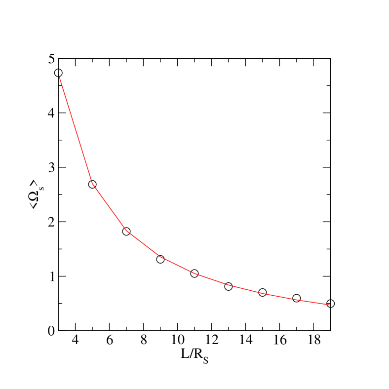
Figure 11: Mean angular velocity versus the length of the spherocylinder with $\alpha_{+}=1$, $\alpha_{-}=0.25$, and spherocylinder mass $M_{S}=40m$.

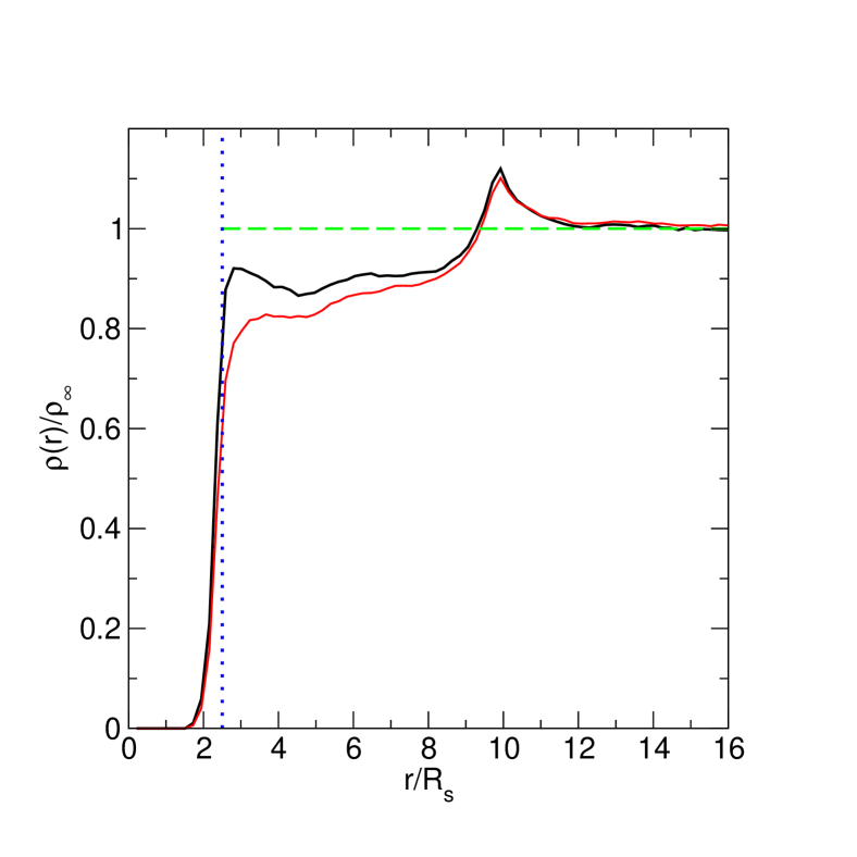
Figure 12: Dimensionless density of the bath particles (second layer) versus the dimensionless distance to the spherocylinder center $r/R_{s}$, with a bath density corresponding to a two-dimensional coverage of 0.18. The bath particle radius is $R=1.5R_{s}$. The black and red curves correspond to homogeneous ($\alpha=0.2$) and heterogeneous ($\alpha_{+}=0.8,\alpha_{-}=0.2$) spherocylinders, respectively. The total length of the spherocylinder is $L+R_{s}=16R_{s}$, The dashed line represents the Boltzmann-Lorentz assumption of a perfect homogeneous bath.

7 Conclusion

We have applied kinetic theory and realistic numerical simulation to study the properties of a chiral heterogeneous granular motor. As with the previously studied piston, a strong ratchet effect may be produced under certain conditions. We also developed a mechanical analysis that provides an exact description in the Brownian limit where the motor is much more massive than a bath particle.

The mechanical approach may also be used to assess the robustness of the ratchet effect. In an experimental situation, a dry friction force between the rotor axle and its bearing is present. If the force or torque acting on a stationary motor exceeds the static friction, the motor effect should be present. In their experiment Eshuis et al.[12] observed that there is a net rotation of the asymmetric vanes that is only non-zero if the bath particles are sufficiently agitated. This is consistent with our analysis that gives an expression for the torque acting on a stationary rotor, equation (36). If this is larger than the static friction, the rotor starts to turn. If the rotor is immobile the granular temperature of the bath particles can be increased by increasing the vibration amplitude or frequency until the threshold is reached.

Eshuis et al.[12] also observed a convective motion that accompanies the motor rotation. This is different from the effect observed in a system of vertically vibrated glass beads where a toroidal convection roll with a vertical axis appears[27]. The origin of this effect is the inelastic collisions between particles and side wall[28]. In the experiment of Eshuis et al., however, convection accompanies the rotation of the vanes and is not the origin of the motor effect.

A more quantitative analysis of the influence of dry friction on the ratchet effect requires its incorporation in the kinetic description. We are currently pursuing this direction.

We thank J. Piasecki for useful discussions.

References

References

- [1] M.v. Smoluchowski. Experimental proof of regular thermodynamics conflicting with molecular phenomena. Physik. Zeitschr, 13:1069, 1912.
- [2] R.B. Leighton R.P. Feynman and M. Sands, editors. The Feynman Lectures on Physics. Addison-Wesley, 1963.
- [3] Peter Reimann. Brownian motors: noisy transport far from equilibrium. Phys. Rep., 361(2-4):57 – 265, 2002.
- [4] M. van den Broek and C. Van den Broeck. Rectifying the thermal brownian motion of three-dimensional asymmetric objects. Phys. Rev. E, 78(1):011102, 2008.
- [5] M. van den Broek, R. Eichhorn, and C. Van den Broeck. Intrinsic ratchets. EPL (Europhysics Letters), 86(3):30002 (6pp), 2009.
- [6] B. Cleuren and C. Van den Broeck. Granular brownian motor. Europhys. Lett., 77(5):50003, 2007.
- [7] G. Costantini, U. Marini Bettolo Marconi, and A. Puglisi. Noise rectification and fluctuations of an asymmetric inelastic piston. Europhys. Lett., 82(5):50008, 2008.
- [8] G. Costantini, A. Puglisi, and U.M.B. Marconi. Granular ratchets. The European Physical Journal - Special Topics, 179:197–206, 2009. 10.1140/epjst/e2010-01203-6.
- [9] Bart Cleuren and Ralf Eichhorn. Dynamical properties of granular rotors. J. Stat. Mech., 2008(10):P10011, 2008.
- [10] P. Viot, A. Burdeau, and J. Talbot. Strong eatchet effects for heterogeneous granular particles in the brownian limit. In 11th Granada Seminar, 2010.
- [11] Giulio Costantini, Umberto Marini Bettolo Marconi, and Andrea Puglisi. Granular brownian ratchet model. Phys. Rev. E, 75(6):061124, 2007.
- [12] Peter Eshuis, Ko van der Weele, Detlef Lohse, and Devaraj van der Meer. Experimental realization of a rotational ratchet in a granular gas. Phys. Rev. Lett., 104(24):248001, 2010.
- [13] Julian Talbot, Alexis Burdeau, and Pascal Viot. Analysis of a class of granular motors in the brownian limit. Phys. Rev. E, 82(1):011135, Jul 2010.
- [14] F. L. Curzon and B. Ahlborn. Efficiency of a carnot engine at maximum power output. Am. J. Phys., 43(1):22–24, 1975.
- [15] C. Van den Broeck. Thermodynamic efficiency at maximum power. Phys. Rev. Lett., 95(19):190602, 2005.
- [16] Frank Jülicher, Armand Ajdari, and Jacques Prost. Modeling molecular motors. Rev. Mod. Phys., 69(4):1269–1282, 1997.
- [17] T. Schmiedl and U. Seifert. Efficiency at maximum power: An analytically solvable model for stochastic heat engines. Europhys. Lett., 81(2):20003, 2008.
- [18] J. Piasecki, J. Talbot, and P. Viot. Angular velocity distribution of a granular planar rotator in a thermalized bath. Phys. Rev. E, 75(5):051307, 2007.
- [19] G. W. Baxter and J. S. Olafsen. Kinetics: Gaussian statistics in granular gases. Nature, 425(6959):680–680, 2003.
- [20] G. W. Baxter and J. S. Olafsen. Experimental evidence for molecular chaos in granular gases. Phys. Rev. Lett., 99(2):028001, 2007.
- [21] G. Bird. Molecular gas dynamics and the direct simulation of gas flows. Clarendon Press, Oxford, England, 1994.
- [22] J. M. Montanero and A. Santos. Computer simulation of uniformly heated granular fluids. Granular Matter, 2:53, 2000.
- [23] J Talbot and P Viot. Application of the gillespie algorithm to a granular intruder particle. Journal of Physics A: Mathematical and General, 39(35):10947, 2006.
- [24] Alexis Burdeau and Pascal Viot. Quasi-gaussian velocity distribution of a vibrated granular bilayer system. Phys. Rev. E, 79(6):061306, Jun 2009.
- [25] P.A. Cundall and O.D.L. Strack. A discrete numerical model for granular assemblies. Geotechnique, 29:47, 1979.
- [26] H. Gomart, J. Talbot, and P. Viot. Boltzmann equation for a granular capped rectangle in a thermalized bath of hard disks. Phys. Rev. E, 71:051306, 2005.
- [27] R. D. Wildman, J. M. Huntley, and D. J. Parker. Granular temperature profiles in three-dimensional vibrofluidized granular beds. Phys. Rev. E, 63:061311, 2001.
- [28] J. Talbot and P. Viot. Wall-Enhanced Convection in Vibrofluidized Granular Systems. Phys. Rev. Lett., 89:064301, 2002.