Electromagnetic Green’s function for layered systems: Applications to nanohole interactions in thin metal films

Abstract

We derive expressions for the electromagnetic Green’s function for a layered system using a transfer matrix technique. The expressions we arrive at makes it possible to study symmetry properties of the Green’s function, such as reciprocity symmetry, and the long-range properties of the Green’s function which involves plasmon waves as well as boundary waves, also known as Norton waves. We apply the method by calculating the light scattering cross section off a chain of nanoholes in a thin Au film. The results highlight the importance of nanohole interactions mediated by surface plasmon propagating along the chain of holes.

I Introduction

The research field of plasmonicsBarnes:03 has seen an enormous development over the last decades, both experimentally and theoretically. Examples of the aspects studied include enhanced light emission under various circumstances,Gimzewski:1989 ; *Berndt:1991; *Qiu:Ho:2003; *Dong:2004; *Schneider:Berndt:2010 enhanced spectroscopies such as surface-enhanced Raman scattering (SERS),Nie:Emory:1997 ; *Kneipp:1997; *Xu:Kall:1999; *Michaels:Brus:1999 extraordinary transmission of lightEbbesen:98 , and biosensing applications.Dahlin:Hook:2005

A corresponding development has also taken place on the theory side and a variety of methods are used to solve theoretical problems in plasmonics. These include exact methods that apply for certain geometries such as Mie theoryWaterman:71 ; Abajo:99 ; Xu:Mie:03 ; Johansson:05 for problems with spherical symmetry, but in most situations methods that make more extensive use of numerical calculations are needed. The finite-difference in time-domain method (FDTD)Yee:FDTD:66 ; Chan:FDTD:95 ; Ward:98 ; Oubre:FDTD:04 is one such method that has grown in popularity in recent years, the discrete-dipole approximation (DDA) methodDraine:94 ; Purcell:73 and Green’s function (GF) methodMartin:JOSA:94 ; Martin:GF:95 ; Paulus:00 ; Nikitin:2008 ; Jung:2008 ; Simsek:2010 are two other methods that are often used. Of these the DDA method has a somewhat longer history and probably a bigger user base. The Green’s function method on the other hand can be more flexible in certain situations.

In this paper we will present a calculation of the Green’s function for a layered material. In particular this makes it possible to study scattering off embedded inclusions such as nanoholes in metal films. Tomas:hole:07 ; Alaverdyan:hole:natphys:07 ; Abajo:RMP07 ; Park:ACSNano:08 ; Sepulveda:OptEx:2008 ; Alegret:NJP:2008 ; Lee:Nordlander:09 ; Vesseur:Abajo:2009 Paulus et al. presented a derivation of the Green’s function (Green’s tensor) for a layered system in Ref. Paulus:00, . The present derivation follows the same basic ideas, but we derive rather elegant, explicit expressions for the Green’s function that only involve a single transfer matrix recursion relation, and which makes it possible to explicitly demonstrate various symmetry properties of the Green’s function such as reciprocity symmetry. We also study the analytic properties of the Green’s function in Fourier space and show how this effects the long-range properties of the Green’s function which for metallic films are dominated by plasmon polaritons for distances typically in the range of 100 nm to 10 $\mathrm{\,\mu m}$ and for even larger distance the dominating contribution comes from a boundary wave.

We will illustrate the Green’s function method by calculating scattering cross sections for light off nanohole systems in thin metal films. The nanoholes of these systems typically have diameters that range from 50 to 100 nm in a thin Au film of thickness 20 nm. The optical properties of nanohole system have attracted intense interest for over a decade now in the context of extraordinary transmission through an array of nanoholes discovered by Ebbesen and coworkers,Ebbesen:98 and studied by various theoretical methods; Porto:Pendry:PRL1999 ; MartinMoreno:2001 for a couple of recent reviews on this subject see Refs. GarciaVidal:10, ; Gordon:Brolo:2010, . But nanohole systems are also studied in connection with biosensing applications, since they at the same time can act as capturing centers for biomolecules and light scatterers whose properties are modulated by the presence of these molecules. The basic optical scattering properties of individual nanoholes and chains of nanoholes in thin metal (Au films) have been studied by Käll and co-workers and the results show signs of strong hole-hole interactions.Alaverdyan:hole:natphys:07 Here we present theoretical results for the scattering cross section off multi-hole systems that are in good agreement with the experimental ones. The theoretical results combined with an analysis of the behavior of the Green’s function shows that the hole-hole interaction affecting the light scattering is to a large extent mediated by surface (interface) plasmons. The special nature of the plasmons means that there is a strong relation between polarization and propagation direction; hole-hole interactions are much stronger in the case when the electric field is polarized along the axis through the hole centers than when the polarization is perpendicular to the chain axis.

The rest of the paper is organized in the following way. In section II we give a brief overview of the Green’s function method. Section III details our calculation of the Green’s function for a layered background through a transfer-matrix method and we also show how a number of physical quantities can be derived from the Green’s function. Section IV focuses on the analytic properties of the Green’s function in wave vector space and its consequences for the long range behavior in real space. Section V gives a brief description of the numerical solution of the integral equation determining the electric field in the scatterers. In Sec. VI we apply the method to a study of the optical properties of nanoholes in a thin metal film, and the paper is summarized in Sec. VII.

II Basic treatment of the scattering problem

We consider first a situation where all of space is filled with a material with dielectric function $\varepsilon_{B}$, corresponding to a wave number

$$k_{B}=\sqrt{\varepsilon_{B}}k_{0}=\sqrt{\varepsilon_{B}}(\omega/c),$$ (1)

where $k_{0}$ and $c$ are the wave number and speed of light in vacuum, respectively, and $\omega$ the angular frequency of electric and magnetic fields. The task at hand is to solve Maxwell’s equations which assuming all fields have a $e^{-i\omega t}$ time dependence, read

$$\nabla\times\vec{E}=i\omega\vec{B},$$ (2)

$$\nabla\times B=\mu_{0}\vec{j}-i\omega\mu_{0}\varepsilon_{0}\varepsilon_{B}\vec{E},$$ (3)

along with

$$\nabla\cdot\vec{B}=0,\ \ \mathrm{and}\ \ \nabla\cdot\vec{D}=\rho.$$ (4)

The solution for the electric field can in this case be written as the sum of a source term that depends on the current at the field point $\vec{r}$ and another term that through a Green’s function takes into account the effects of the currents everywhere else,Yaghjian:80

$$\vec{E}(\vec{r})=\frac{\tensor{L}\cdot\vec{j}(\vec{r})}{i\omega\varepsilon_{0}\varepsilon_{B}}+i\omega\mu_{0}\int_{V_{j}-V_{\delta}}\tensor{G}_{h}(\vec{r},\vec{r}^{\prime})\cdot\vec{j}(\vec{r}^{\prime})d^{3}r^{\prime}.$$ (5)

Here $\tensor{L}$ is a tensor which depends on the shape of the excluded volume $V_{\delta}$. In the most common cases where the excluded volume is cubic or spherical in shape $\tensor{L}$ is diagonal and each of its three elements have the value 1/3. The Green’s function is given by

$$\tensor{G}_{h}(\vec{r},\vec{r^{\prime}})=\left[\tensor{1}+\frac{\nabla\nabla}{k_{B}^{2}}\right]G^{\mathrm{s}}(\vec{r},\vec{r^{\prime}})=\left[\tensor{1}+\frac{\nabla\nabla}{k_{B}^{2}}\right]\frac{e^{ik_{B}|\vec{r}-\vec{r^{\prime}}|}}{4\pi|\vec{r}-\vec{r^{\prime}}|},$$ (6)

where $G^{\mathrm{s}}$ is the Green’s function to the scalar Helmholtz equation, and thus satisfies

$$(\nabla^{2}+k_{B}^{2})G^{\mathrm{s}}(\vec{r},\vec{r^{\prime}})=-\delta^{(3)}(\vec{r}-\vec{r}^{\prime}).$$ (7)

More explicitly we have

$$\tensor{G}_{h}(\vec{R}) =\left(\tensor{1}+\frac{ik_{B}R-1}{k_{B}^{2}R^{2}}\tensor{1}\right.$$ (8)

$$\left.+\frac{3-3ik_{B}R-k_{B}^{2}R^{2}}{k_{B}^{2}R^{4}}\vec{R}\otimes\vec{R}\right)\frac{e^{ik_{B}R}}{4\pi R},$$

where $\vec{R}=\vec{r}-\vec{r^{\prime}}$, and $\otimes$ denotes a dyadic product.

In case the dielectric function is not constant in space, there is a modification of the second of the Maxwell’s equations

$$\nabla\times\vec{B}=\mu_{0}\vec{j}-\frac{i\omega\varepsilon_{B}}{c^{2}}\vec{E}-\frac{i\omega(\varepsilon_{\mathrm{rel}}-\varepsilon_{B})}{c^{2}}\vec{E},$$ (9)

where the last term is new compared with the case of a homogeneous medium, and $\varepsilon_{\mathrm{rel}}$ can vary in space in an essentially arbitrary way. We rewrite this as

$$\nabla\times\vec{B}=\mu_{0}\vec{j}_{\mathrm{tot}}-\frac{i\omega\varepsilon_{B}}{c^{2}}\vec{E}$$ (10)

where the total current due to both external sources and scattering is

$$\vec{j}_{\mathrm{tot}}=\vec{j}+\vec{j}_{\mathrm{scatt}}=\vec{j}-\frac{1}{\mu_{0}}\frac{i\omega(\varepsilon_{\mathrm{rel}}-\varepsilon_{B})}{c^{2}}\vec{E}.$$ (11)

By letting $\vec{j}_{\mathrm{tot}}$ take the place of $\vec{j}$ in the solution we get

$$\vec{E}(\vec{r}) =\frac{\tensor{L}\cdot\vec{j}(\vec{r})}{i\omega\varepsilon_{0}\varepsilon_{B}}-\frac{\Delta\varepsilon(\vec{r)}}{\varepsilon_{B}}\tensor{L}\cdot\vec{E}(\vec{r})+\int_{V_{j}-V_{\delta}}\tensor{G}_{h}(\vec{r},\vec{r}^{\prime})$$ (12)

$$\times\left(i\omega\mu_{0}\vec{j}(\vec{r}^{\prime})+k_{0}^{2}\Delta\varepsilon(\vec{r^{\prime}})\vec{E}(\vec{r^{\prime}})\right)d^{3}r^{\prime}.$$

We will next show how this expression, in particular the Green’s function, can be generalized to deal with a layered system where the background dielectric function $\varepsilon_{B}(\vec{r})$ varies stepwise along one direction ($z$) in space, and $\Delta\varepsilon=\varepsilon_{\mathrm{rel}}-\varepsilon_{B}$ then describes further variations of the dielectric function due to scatterers.

III Green’s function for a layered structure

III.1 Formulation in terms of 2D Fourier transform

The Green’s function for a homogeneous background given above in Eq. (6) can be written in terms of a Fourier integral as

$$\tensor{G}_{h}(\vec{R})=\int\frac{d^{3}q}{(2\pi)^{3}k_{B}^{2}}\frac{k_{B}^{2}\tensor{1}-\vec{q}\otimes\vec{q}}{q^{2}-k_{B}^{2}}e^{i\vec{q}\cdot\vec{R}}.$$ (13)

This expression becomes more useful in handling layered structures if we integrate out the $q_{z}$ variable, which yieldsPaulus:00

$$\tensor{G}_{h}(\vec{R})=-\frac{\hat{z}\otimes\hat{z}}{k_{B}^{2}}\delta^{(3)}(\vec{R})+\int\frac{d^{2}q}{(2\pi)^{2}}\tensor{G}_{h}(\vec{q}_{\|},z)e^{i\vec{q}_{\|}\cdot\vec{r}_{\|}}.$$ (14)

The notation $\tensor{G}_{h}$ indicates that we are still dealing with the Green’s function for a homogeneous background, but the formal generalization of Eq. (14) to $\tensor{G}$ valid for a layered background is straightforward. The $\delta$-function term is the result of a subtract-add operation necessary to render the contour integral convergent. However, in the following we will not explicitly deal with the singular behavior of $\tensor{G}$ when $\vec{r}\to\vec{r}^{\prime}$, so we will therefore leave out this term in the rest of the calculation. The 2D Fourier transform (FT) of the Green’s function in Eq. (14) is

$$\tensor{G}_{h}(\vec{q}_{\|},z,z^{\prime})=\frac{i}{2p}\left(\tensor{1}-\frac{\vec{q}^{\,\tau}\otimes\vec{q}^{\,\tau}}{k_{B}^{2}}\right)e^{ip|z-z^{\prime}|},$$ (15)

where $p$ stands for the absolute value of the $z$ component of the wave vector $\vec{q}$ (originating from the residue at the pole in the contour integration)

$$p=\sqrt{k_{B}^{2}-|\vec{q}_{\|}|^{2}}.$$ (16)

The square root function in Eq. (16) should, to give physical results in the form of outgoing, damped waves, be evaluated with the branch cut along the positive real axis of the argument. The superscript $\tau$ on the wave vector $\vec{q}^{\,\tau}$ indicates the direction of propagation of the waves (called primary propagation direction in the following) $\tau=+1$, or just $\tau=+$, when $z>z^{\prime}$ and $\tau=-1$ when $z<z^{\prime}$. For the wave vectors we have

$$\vec{q}^{\pm}=\vec{q}_{\|}\pm p\hat{z}.=((q_{\|}/k_{B})\cos{\phi_{q}},(q_{\|}/k_{B})\sin{\phi_{q}},\pm p/k_{B}),$$ (17)

where $q_{\|}=|\vec{q}_{\|}|$. The corresponding unit vector,

$$\hat{q}^{\,\tau}=\vec{q}^{\,\tau}/k_{B},$$ (18)

together with the unit polarization vectors for s polarization

$$\hat{s}^{\pm}=\frac{\hat{z}\times\hat{q}^{\pm}}{|\hat{z}\times\hat{q}^{\pm}|}=(-\sin{\phi_{q}},\cos{\phi_{q}},0),$$ (19)

and p polarization

$$\hat{p}^{\pm}=\hat{s}^{\pm}\times\hat{q}^{\pm}=\left(\pm\frac{p}{k_{B}}\cos{\phi_{q}},\pm\frac{p}{k_{B}}\sin{\phi_{q}},-\frac{q_{\|}}{k_{B}}\right),$$ (20)

form an orthonormal basis. The unit tensor therefore can be written

$$\tensor{1}=\hat{q}^{\tau}\otimes\hat{q}^{\tau}+\hat{p}^{\tau}\otimes\hat{p}^{\tau}+\hat{s}^{\tau}\otimes\hat{s}^{\tau}.$$ (21)

Using Eqs. (18) and (21) we can rewrite the Green’s function Fourier transform in Eq. (15) as

$$\tensor{G}_{h}(\vec{q}_{\|},z,z^{\prime})=\frac{i}{2p}\left(\hat{p}^{\tau}\otimes\hat{p}^{\tau}+\hat{s}^{\tau}\otimes\hat{s}^{\tau}\right)e^{i\tau p(z-z^{\prime})}.$$ (22)

As a first step towards generalizing Eq. (22) to a situation with a layered background, we conclude that a particular element of the tensor can be written

$$G_{h,\alpha\beta}(\vec{q}_{\|},z,z^{\prime})=\hat{\alpha}\cdot\vec{\mathcal{E}}=$$

$$=\hat{\alpha}\cdot\left[(\hat{p}^{\tau}A^{\tau,p}+\hat{s}^{\tau}A^{\tau,s})e^{i\tau p(z-z^{\prime})}\right],$$ (23)

where $\vec{\mathcal{E}}$ is a vector field proportional to an electric field generated by the source. The wave amplitudes are found by projecting the source unit vector $\hat{\beta}$ onto the p and s unit vectors, thus

$$A^{\tau,p}=\frac{i}{2p}\,\hat{p}^{\tau}\cdot\hat{\beta}\ \ \ \ \mathrm{and}\ \ \ \ A^{\tau,s}=\frac{i}{2p}\,\hat{s}^{\tau}\cdot\hat{\beta}.$$ (24)

III.2 Generalization to a layered material

When we turn to a layered material the source will still generate outgoing plane waves just like the expression in Eq. (23) indicates, however, now there will also be other waves reflected and transmitted at the different interfaces.

Figure 1: Illustration of the plane waves generated in the different layers of a four-layer system when the source is placed at $z=z^{\prime}$.

This is illustrated in Fig. 1. for a system with four layers and the source placed in layer 3. In layer 3, there are waves going upwards and downwards on both sides of the source, in layer 2 there are also waves propagating in both directions, but in the two outermost layers there are only outgoing waves, propagating upwards in layer 1 and downwards in layer 4. The vector field $\vec{\mathcal{E}}$ we introduced in Eq. (23) takes the generalized form

$$\vec{\mathcal{E}}=\left[\left(\hat{p}_{l}^{\tau}A_{l}^{\tau,p}(z_{0,l})+\hat{s}A_{l}^{\tau,s}(z_{0,l})\right)e^{i\tau p_{l}(z-z_{0,l})}\right.$$

$$\left.+\left(\hat{p}_{l}^{\overline{\tau}}B_{l}^{\tau,p}(z_{0,l})+\hat{s}B_{l}^{\tau,s}(z_{0,l})\right)e^{-i\tau p_{l}(z-z_{0,l})}\right],$$ (25)

in layer $l$. Here $\overline{\tau}$ is the opposite direction of $\tau$, $-\tau$, and the unit vectors for p polarization as well as $p$ depends on the layer number $l$ since the background wave vector magnitude $k_{B}$ varies from layer to layer. The wave amplitudes $A_{l}^{\tau,\sigma}(z_{0,l})$ for outgoing waves propagating away from $z=z^{\prime}$ and $B_{l}^{\tau,\sigma}(z_{0,l})$ for returning waves propagating towards $z=z^{\prime}$ in Eq. (25) depend on the layer number $l$, primary propagation direction $\tau$, and polarization $\sigma$ (p or s). The offset points $z_{0,l}$ are local origins for the plane wave exponentials, which can be moved around provided, of course, that the wave amplitudes are adjusted accordingly. The standard choice for $z_{0,l}$, in particular in a numerical implementation, is to use the bottom of all the layers above the source, and the top of all the layers below the source. In Fig. 1 this means that $z_{0,1}=d_{1}$, $z_{0,2}=d_{2}$, $z_{0,3}=z^{\prime}$, and $z_{0,4}=d_{3}$.

We need to determine the wave amplitudes $A_{l}^{\tau,\sigma}(z_{0,l})$ and $B_{l}^{\tau,\sigma}(z_{0,l})$, something we will do in two steps. First we view the stack of layers as made up of two independent parts, one above the source plane $z=z^{\prime}$, and one below. We introduce relative wave amplitudes $a_{l}^{\tau,\sigma}(z_{0,l})$ and $b_{l}^{\tau,\sigma}(z_{0,l})$, corresponding to the actual amplitudes $A_{l}^{\tau,\sigma}(z_{0,l})$ and $B_{l}^{\tau,\sigma}(z_{0,l})$. The actual amplitudes above the source are found from the relative ones as

$$A_{l}^{+}(z^{\prime\prime})=\frac{a_{l}^{+}(z^{\prime\prime})}{a_{l^{\prime}}^{+}(z^{\prime})}A_{l^{\prime}}^{+}(z^{\prime}),\ \ \ \ B_{l}^{+}(z^{\prime\prime})=\frac{b_{l}^{+}(z^{\prime\prime})}{a_{l^{\prime}}^{+}(z^{\prime})}A_{l^{\prime}}^{+}(z^{\prime}),$$ (26)

where $l^{\prime}$ denotes the source layer and $z^{\prime\prime}$ is any $z$ coordinate. In the same way, below the source

$$A_{l}^{-}(z^{\prime\prime})=\frac{a_{l}^{-}(z^{\prime\prime})}{a_{l^{\prime}}^{-}(z^{\prime})}A_{l^{\prime}}^{-}(z^{\prime}),\ \ \ \ B_{l}^{-}(z^{\prime\prime})=\frac{b_{l}^{-}(z^{\prime\prime})}{a_{l^{\prime}}^{-}(z^{\prime})}A_{l^{\prime}}^{-}(z^{\prime}).$$ (27)

The relative amplitudes can be determined by a transfer-matrix calculation using the fact that there are only outgoing waves in the outermost layers. But Eqs. (26) and (27) show that the actual wave amplitudes $A_{l^{\prime}}^{+}$ and $A_{l^{\prime}}^{-}$ in the source layer play the role of driving forces for all the waves above and below the source, respectively, and still have to be calculated independently. This is done in the second step of our calculation, by a detailed investigation of the situation in the source layer.

III.3 Transfer matrix calculation

The calculation of the relative amplitudes uses the fact that there are no returning waves in the outermost layers, thus

$$B_{1}^{+}=b_{1}^{+}=0,\ \ \ \mathrm{and}\ \ \ B_{N}^{-}=b_{N}^{-}=0.$$ (28)

We set the relative amplitudes of the outgoing waves in the outermost layers, i.e. $a_{1}^{+}$ and $a_{N}^{-}$, to 1,

$$a_{1}^{+}(z_{+})=1,\ \ \ \mathrm{and}\ \ \ a_{N}^{-}(z_{-})=1.$$ (29)

The coordinates $z_{+}$ and $z_{-}$ lie above ($z_{+}$) and below ($z_{-}$) all interfaces as well as the source and field points, respectively.

The remaining relative amplitudes can then be determined by recursion, applying the Fresnel formula at each interface and adjusting the amplitudes by exponentials to account for the propagation through intermediate layers. For a general $z$ coordinate $z^{\prime\prime}$ we get

$$\left[\begin{array}[]{c}a_{l}^{+,\sigma}(z^{\prime\prime})\\ b_{l}^{+,\sigma}(z^{\prime\prime})\\ \end{array}\right]=W^{+}(z^{\prime\prime},z_{+})\left[\begin{array}[]{c}1\\ 0\\ \end{array}\right]$$ (34)

$$=S_{l}^{+}(z^{\prime\prime},d_{l-1})T_{l,l-1}^{+,\sigma}\cdots T_{2,1}^{+,\sigma}S_{1}^{+}(d_{1},z_{+})\left[\begin{array}[]{c}1\\ 0\\ \end{array}\right]$$ (37)

above the source, and

$$\left[\begin{array}[]{c}a_{l}^{-,\sigma}(z^{\prime\prime})\\ b_{l}^{-,\sigma}(z^{\prime\prime})\\ \end{array}\right]=W^{-}(z^{\prime\prime},z_{-})\left[\begin{array}[]{c}1\\ 0\\ \end{array}\right]=$$ (42)

$$=S_{l}^{-}(z^{\prime\prime},d_{l})T_{l,l+1}^{-,\sigma}\cdots T_{N-1,N}^{-,\sigma}S_{N}^{-}(d_{N-1},z_{-})\left[\begin{array}[]{c}1\\ 0\\ \end{array}\right]$$ (45)

below the source. Here $W$ is a “total” transfer matrix built up by factors $S$, related to the wave propagation in the different layers, and $T$, describing reflection and transmission at a particular interface.

The propagation in one single layer just yields exponential factors multiplying the wave amplitudes. We have

$$\left[\begin{array}[]{c}a_{l}^{\tau,\sigma}(z)\\ b_{l}^{\tau,\sigma}(z)\\ \end{array}\right]=S_{l}^{\tau}(z,z^{\prime\prime})\left[\begin{array}[]{c}a_{l}^{\tau,\sigma}(z^{\prime\prime})\\ b_{l}^{\tau,\sigma}(z^{\prime\prime})\\ \end{array}\right],$$ (46)

where $\sigma$ denotes a polarization (s or p) and where

$$S_{l}^{\pm}(z,z^{\prime\prime})=\left[\begin{array}[]{cc}e^{\pm ip_{l}(z-z^{\prime\prime})}&0\\ 0&e^{\mp ip_{l}(z-z^{\prime\prime})}\\ \end{array}\right].$$ (47)

The cross-interface transfer matrices $T$ relate the wave coefficients on opposite sides of an interface $z=d$, separating layers $l$ and $n$ (where $l=n\pm 1$), to each other

$$\left[\begin{array}[]{c}a_{l}^{\tau,\sigma}(d)\\ b_{l}^{\tau,\sigma}(d)\\ \end{array}\right]=T_{ln}^{\tau,\sigma}\left[\begin{array}[]{c}a_{n}^{\tau,\sigma}(d)\\ b_{n}^{\tau,\sigma}(d)\\ \end{array}\right].$$ (48)

They can be evaluated by using the Fresnel formulae for s and p polarized waves. We express the result in terms of the reflection amplitudes for $s$ and $p$ polarized waves, respectively, incident from the material in layer $l$ onto material $n$ in case this is the only interface,

$$f_{ln}^{s}=\frac{p_{l}-p_{n}}{p_{l}+p_{n}}\ \ \ \mathrm{and}\ \ \ f_{ln}^{p}=\frac{\varepsilon_{n}p_{l}-\varepsilon_{l}p_{n}}{\varepsilon_{n}p_{l}+\varepsilon_{l}p_{n}}.$$ (49)

These quantities depend on the dielectric functions $\varepsilon_{l}$ and $\varepsilon_{n}$ and wave vector $z$ components $p_{l}$ and $p_{n}$ of the two layers. The $T$ matrices are found after some algebra which also involves the amplitude of the transmitted wave. We get

$$T_{ln}^{\tau s}=\frac{1}{1+f_{ln}^{s}}\left[\begin{array}[]{cc}1&f_{ln}^{s}\\ f_{ln}^{s}&1\end{array}\right]$$ (50)

for s polarization, and

$$T_{ln}^{\tau p}=\frac{k_{l}p_{n}}{k_{n}p_{l}}\frac{1}{1-f_{ln}^{p}}\left[\begin{array}[]{cc}1&f_{ln}^{p}\\ f_{ln}^{p}&1\end{array}\right]$$ (51)

for p polarization.

III.4 Calculation of the primary wave

Using the scheme outlined in Sec. III.3 we can calculate all the relative wave amplitudes we need. Now it remains to find the primary wave amplitudes $A_{l^{\prime}}^{\pm,\sigma}$ in the source layer. We have already seen that in the case of a homogeneous material we have

$$A_{l^{\prime}}^{\tau,p}(z^{\prime})=\frac{i}{2p_{l^{\prime}}}\,\hat{p}^{\tau}\cdot\hat{\beta}\ \ \ \ \mathrm{and}\ \ \ \ A_{l^{\prime}}^{\tau,s}(z^{\prime})=\frac{i}{2p_{l^{\prime}}}\,\hat{s}^{\tau}\cdot\hat{\beta}.$$ (52)

In the present case we have to add the wave reflected off the “opposite” interface of the source layer to each of these expressions. Thus, the amplitude of the wave propagating upwards has a direct contribution from the source, and one contribution from the interface below the source, and vice versa for the wave propagating downwards. By introducing the response functions, i.e. the ratios between reflected and incident wave amplitudes,

$$\chi^{\tau,\sigma}(z^{\prime\prime})=\frac{b_{l}^{\tau,\sigma}(z^{\prime\prime})}{a_{l}^{\tau,\sigma}(z^{\prime\prime})}=\frac{B_{l}^{\tau,\sigma}(z^{\prime\prime})}{A_{l}^{\tau,\sigma}(z^{\prime\prime})}$$ (53)

we can write (using $\hat{\sigma}$ as a general polarization vector, $\hat{s}$ or $\hat{p}$) each of these amplitudes as

$$A_{l^{\prime}}^{\tau,\sigma}(z^{\prime})=\frac{i}{2p_{l^{\prime}}}\,\hat{\sigma}_{l^{\prime}}^{\tau}\cdot\hat{\beta}+\chi^{\overline{\tau},\sigma}(z^{\prime})A_{l^{\prime}}^{\overline{\tau},\sigma}(z^{\prime}),\ \ \tau=\pm 1.$$ (54)

This system of two equations has the solution

$$A_{l^{\prime}}^{\tau,\sigma}(z^{\prime})=\frac{(\hat{\sigma}_{l^{\prime}}^{\tau}+\hat{\sigma}_{l^{\prime}}^{\overline{\tau}}\,\chi^{\overline{\tau},\sigma}(z^{\prime}))\cdot\hat{\beta}}{1-\chi^{+,\sigma}(z^{\prime})\chi^{-,\sigma}(z^{\prime})}\,\frac{i}{2p_{l^{\prime}}}$$ (55)

in which the first term in the numerator is the direct wave from the source, the second term is the wave reflected once off the opposite interface, and the denominator accounts for repeated reflections off the surrounding interfaces. We can now calculate the Green’s function by using this solution in Eqs. (25), (26), and (27).

III.5 Results for the Fourier-space GF

With a source pointing in the $\beta$ direction we can now write down the result for the matrix element $G_{\alpha\beta}(\vec{q}_{\|},z,z^{\prime})=\hat{\alpha}\cdot\mathcal{E}$ in Fourier space. To keep the whole thing manageable we divide the Green’s function into one p part and one s part

$$\tensor{G}(\vec{q}_{\|},z,z^{\prime})=\tensor{G}^{p}(\vec{q}_{\|},z,z^{\prime})+\tensor{G}^{s}(\vec{q}_{\|},z,z^{\prime}),$$ (56)

with

$$\tensor{G}^{p}(\vec{q}_{\|},z,z^{\prime})=\left[\hat{p}_{l}^{\tau}\,\frac{a_{l}^{\tau,p}(z_{0,l})}{a_{l^{\prime}}^{\tau,p}(z^{\prime})}e^{i\tau p_{l}(z-z_{0,l})}+\hat{p}_{l}^{\overline{\tau}}\,\frac{b_{l}^{\tau,p}(z_{0,l})}{a_{l^{\prime}}^{\tau,p}(z^{\prime})}e^{-i\tau p_{l}(z-z_{0,l})}\right]\otimes\frac{(\hat{p}_{l^{\prime}}^{\tau}+\chi^{\overline{\tau},p}(z^{\prime})\hat{p}_{l^{\prime}}^{\overline{\tau}})}{1-\chi^{+,p}(z^{\prime})\chi^{-,p}(z^{\prime})}\,\frac{i}{2p_{l^{\prime}}}$$ (57)

and

$$\tensor{G}^{s}(\vec{q}_{\|},z,z^{\prime})=\left[\frac{a_{l}^{\tau,s}(z_{0,l})}{a_{l^{\prime}}^{\tau,s}(z^{\prime})}e^{i\tau p_{l}(z-z_{0,l})}+\frac{b_{l}^{\tau,s}(z_{0,l})}{a_{l^{\prime}}^{\tau,s}(z^{\prime})}e^{-i\tau p_{l}(z-z_{0,l})}\right]\hat{s}\otimes\hat{s}\,\frac{[1+\chi^{\overline{\tau},s}(z^{\prime})]}{1-\chi^{+,s}(z^{\prime})\chi^{-,s}(z^{\prime})}\,\frac{i}{2p_{l^{\prime}}}.$$ (58)

These expressions are a good starting point for a numerical implementation.

For theoretical purposes it is, however, quite useful to express the Green’s functions in terms of the $W$ transfer matrices. By multiplying the numerators and denominators in Eqs. (57) and (58) by $a_{l^{\prime}}^{\tau,\sigma}(z^{\prime})a_{l^{\prime}}^{\overline{\tau},\sigma}(z^{\prime})$, and using that, in view of Eqs. (37) and (45), $a_{l^{\prime\prime}}^{\tau,\sigma}(z^{\prime\prime})$ and $b_{l^{\prime\prime}}^{\tau,\sigma}(z^{\prime\prime})$ are the first column elements of $W^{\tau,\sigma}(z^{\prime\prime},z_{\tau})$ we arrive at

$$\tensor{G}^{p}(\vec{q}_{\|},z,z^{\prime})=\frac{W_{11}^{\tau,p}(z,z_{\tau})\,\left[\hat{p}_{l}^{\tau}+\hat{p}_{l}^{\overline{\tau}}\chi^{\tau,p}(z)\right]\otimes\left[\hat{p}_{l^{\prime}}^{\tau}+\hat{p}_{l^{\prime}}^{\overline{\tau}}\chi^{\overline{\tau},p}(z^{\prime})\right]\,W_{11}^{\overline{\tau},p}(z^{\prime},z_{\overline{\tau}})}{D_{11}^{p}(z^{\prime})}$$ (59)

and

$$\tensor{G}^{s}(\vec{q}_{\|},z,z^{\prime})=\frac{W_{11}^{\tau,s}(z,z_{\tau})\,\left[1+\chi^{\tau,s}(z)\right]\hat{s}\otimes\hat{s}\left[1+\chi^{\overline{\tau},s}(z^{\prime})\right]\,W_{11}^{\overline{\tau},s}(z^{\prime},z_{\overline{\tau}})}{D_{11}^{s}(z^{\prime})},$$ (60)

where

$$D_{11}^{\sigma}(z^{\prime})=-2ip_{l^{\prime}}\,\left[W_{11}^{+,\sigma}(z^{\prime},z_{+})W_{11}^{-,\sigma}(z^{\prime},z_{-})-W_{21}^{+,\sigma}(z^{\prime},z_{+})W_{21}^{-,\sigma}(z^{\prime},z_{-})\right]$$ (61)

is the $1,1$ element of the matrix

$$D^{\sigma}(z^{\prime})=\left[W^{+,\sigma}(z^{\prime},z_{+})\right]^{t}(-2ip_{l^{\prime}}\sigma_{z})W^{-,\sigma}(z^{\prime},z_{-}).$$ (62)

Here the superscript $t$ denotes matrix transposition, and $\sigma_{z}$ is the Pauli matrix

$$\sigma_{z}=\left[\begin{array}[]{cr}1&0\\ 0&-1\\ \end{array}\right].$$ (63)

To summarize, Eqs. (59)–(61) show how the Green’s function can be uniquely expressed in terms of the transfer matrices describing propagation from the outer layers of the system to the source and field points $z^{\prime}$ and $z$, respectively.

III.6 Calculation of the real-space GF

The layered system we are considering has cylindrical symmetry and it is therefore quite natural to view both the Green’s function in real space, as well as its Fourier transform which has been at the center of our attention so far, as functions of cylindrical coordinates

$$\tensor{G}(\vec{r},\vec{r}^{\prime})\equiv\tensor{G}(\rho,\phi,z,z^{\prime})\ \ \mathrm{and}\ \ \tensor{G}(\vec{q}_{\|},z,z^{\prime})\equiv\tensor{G}(q_{\|},\phi_{q},z,z^{\prime}),$$ (64)

respectively.

Thanks to the cylindrical symmetry the Fourier transform of the Green’s function for an arbitrary $\phi_{q}$ can be related to the one at $\phi_{q}=0$ through

$$\tensor{G}(q_{\|},\phi_{q},z,z^{\prime})=U(\phi_{q})\tensor{G}(q_{\|},\phi_{q}=0,z,z^{\prime})[U(\phi_{q})]^{t},$$ (65)

where

$$U(\phi_{q})=\left[\begin{array}[]{ccc}\cos{\phi_{q}}&-\sin{\phi_{q}}&0\\ \sin{\phi_{q}}&\cos{\phi_{q}}&0\\ 0&0&1\end{array}\right],$$ (66)

and the superscript $t$ denotes transposition. For $\phi_{q}=0$ $\tensor{G}^{p}(q_{\|},0,z,z^{\prime})$ has four non-zero components $xx$, $xz$, $zx$, and $zz$, while for $\tensor{G}^{s}(q_{\|},0,z,z^{\prime})$ only the $yy$ component is non-zero.

Likewise, for $\phi=0$ the Green’s function in real space has 5 non-zero components $xx$, $yy$, $xz$, $zx$, and $zz$ and for a general $\phi$ we have

$$\tensor{G}(\rho,\phi,z,z^{\prime})=U(\phi)\tensor{G}(\rho,\phi=0,z,z^{\prime})[U(\phi)]^{t}.$$ (67)

Therefore to calculate $\tensor{G}(\rho,\phi,z,z^{\prime})$ in practice, we first calculate $\tensor{G}$ for $\phi=0$ using the generalization of Eq. (14) to the case of a layered material and then use Eq. (67) to get the final result. The angular part of the Fourier integral can be carried out analytically by making use of the integral representation of the Bessel functions

$$i^{n}J_{n}(z)=\frac{1}{2\pi}\int_{0}^{2\pi}e^{iz\cos{\phi}}\cos{n\phi}\,d\phi.$$ (68)

We get

$$\tensor{G}(\rho,0,z,z^{\prime})=\int\frac{d^{2}q_{\|}}{(2\pi)^{2}}U(\phi_{q})\tensor{G}(q_{\|},0,z,z^{\prime})[U(\phi_{q})]^{t}e^{i\vec{q}_{\|}\cdot\vec{r}_{\|}}$$

$$=\left[\begin{array}[]{ccc}G_{xx}(\rho,0,z,z^{\prime})&0&G_{xz}(\rho,0,z,z^{\prime})\\ 0&G_{yy}(\rho,0,z,z^{\prime})&0\\ G_{zx}(\rho,0,z,z^{\prime})&0&G_{zz}(\rho,0,z,z^{\prime})\end{array}\right],$$ (72)

and using $e^{i\vec{q}_{\|}\cdot\vec{r}_{\|}}=e^{iq_{\|}\rho\cos{\phi_{q}}}$ and Eq. (68) the different components are explicitly given by

$$G_{xx}(\rho,0,z,z^{\prime})=\int_{0}^{\infty}\left[\left(J_{0}(q_{\|}\rho)-\frac{J_{1}(q_{\|}\rho)}{q_{\|}\rho}\right)\right.$$

$$\left.\times G_{xx}(q_{\|},0,z,z^{\prime})+\frac{J_{1}(q_{\|}\rho)}{q_{\|}\rho}G_{yy}(q_{\|},0,z,z^{\prime})\right]\,\frac{dq_{\|}}{2\pi},$$

(74)

$$G_{xz}(\rho,0,z,z^{\prime})=\int_{0}^{\infty}iJ_{1}(q_{\|}\rho)G_{xz}(q_{\|},0,z,z^{\prime})\,\frac{dq_{\|}}{2\pi},$$ (75)

and

$$G_{zz}(\rho,0,z,z^{\prime})=\int_{0}^{\infty}J_{0}(q_{\|}\rho)G_{zz}(q_{\|},0,z,z^{\prime})\frac{dq_{\|}}{2\pi}.$$ (76)

The expression for $G_{yy}(\rho,0,z,z^{\prime})$ is obtained by the index replacements $xx\to yy$ and $yy\to xx$ in Eq. (74), and $G_{zx}(\rho,0,z,z^{\prime})$ is obtained by replacing the index $xz$ in Eq. (75) by $zx$.

The integrations in Eqs. (74), (75) and (76) nominally run along the real $q_{\|}$ axis, however, as discussed in Ref. Paulus:00, the numerical evaluation can be speeded up by deforming the integration contour into the complex plane. As a first step we also divide the Green’s function into two parts, the homogeneous part $\tensor{G}_{h}$ that we have already discussed and given explicit expressions for, and an indirect part $\tensor{G}_{ind}$.Simsek:2010 The homogeneous part refers to the situation without interfaces; the indirect part contains all contributions to the Greens function that at any point involves the reflection or transmission of a wave at any of the interfaces of the layered system. Both in real space and Fourier space

$$\tensor{G}=\tensor{G}_{h}+\tensor{G}_{ind}.$$ (77)

Thus, in practice we evaluate $\tensor{G}_{h}$ from the explicit expression in Eq. (8), while the indirect part is calculated from the Fourier integrals above. The functions in the respective integrals are analytic in the lower half plane (LHP) but has two branch cuts in the upper half plane (UHP) along the hyperbolas for which $\mathrm{Im}[p_{1}]=0$ and $\mathrm{Im}[p_{N}]=0$, respectively, where $p_{1}$ and $p_{N}$ are given by Eq. (16) using the material properties of the top and bottom layers. In addition the integrands may have one or several poles in the UHP. We deform the integration contour so that it starts from $q_{\|}=0$, first runs along the negative imaginary axis, then goes parallel to the real axis until it reaches a point beyond the singularities in the UHP where it goes back to the real axis. From there the integration either proceeds along the real axis to values of $q_{\|}$ large enough that further contributions are negligible, or in the case that the lateral distance $\rho$ between the source and field points is large a faster convergence is achieved by rewriting the Bessel functions in terms of Hankel functions as Paulus:00

$$J_{n}(q_{\\ }\rho)=\frac{1}{2}\left[H_{n}^{(1)}(q_{\\ }\rho)+H_{n}^{(2)}(q_{\\ }\rho)\right],$$ (78)

and then carrying out the integration of the $H_{n}^{(1)}$ part along a vertical path in the UHP and the $H_{n}^{(2)}$ part along a vertical path in the LHP.

For the purpose of (semi-)analytical calculations of the Green functions it is often an advantage to deform the branch cuts, more about that later.

III.7 Reciprocity symmetry of the Green’s function

Reciprocity, which can be stated as “interchanging the source and the field probe does not change the result,” is a central property of linear, time-reversal-invariant electrodynamics. In our case this requires that the Green’s function fulfills the relation

$${G}_{\beta\alpha}(\vec{r}_{2},\vec{r}_{1})={G}_{\alpha\beta}(\vec{r}_{1},\vec{r}_{2}).$$ (79)

To show that this is in fact true one can go back to Eqs. (59) and (60), and first look at the matrix appearing in the denominators, $D^{\sigma}(z^{\prime})$. While $D^{\sigma}(z^{\prime})$ nominally appears to be a function of the source coordinate $z^{\prime}$, it is in fact an invariant, independent of $z^{\prime}$. To see this we first note that $D^{\sigma}$ is independent of the position of $z^{\prime}$ within layer $l^{\prime}$. Writing $D^{\sigma}$ as

$$D^{\sigma}(z^{\prime})=\left[W^{+,\sigma}(d_{l^{\prime}-1}-0,z_{+})\right]^{t}S_{l^{\prime}}^{+}(z^{\prime},d_{l^{\prime}-1})(-2ip_{l^{\prime}}\sigma_{z})S_{l^{\prime}}^{-}(z^{\prime},d_{l^{\prime}})W^{-,\sigma}(d_{l^{\prime}}+0,z_{-}),$$ (80)

explicitly exposes the propagation in layer $l^{\prime}$ and it is easy to show that

$$S_{l^{\prime}}^{+}(z^{\prime},d_{l^{\prime}-1})(-2ip_{l^{\prime}}\sigma_{z})S_{l^{\prime}}^{-}(z^{\prime},d_{l^{\prime}})=S_{l^{\prime}}^{+}(d_{l^{\prime}},d_{l^{\prime}-1})(-2ip_{l^{\prime}}\sigma_{z})=(-2ip_{l^{\prime}}\sigma_{z})S_{l^{\prime}}^{-}(d_{l^{\prime}-1},d_{l^{\prime}}).$$ (81)

It remains to see what happens to $D^{\sigma}(z^{\prime})$ when $z^{\prime}$ is moved across an interface. We then have

$$D^{\sigma}(d_{l^{\prime}}+0)=\left[W^{+,\sigma}(d_{l^{\prime}}+0,z_{+})\right]^{t}(-2ip_{l^{\prime}}\sigma_{z})T_{l^{\prime},l^{\prime}+1}^{\sigma}W^{-,\sigma}(d_{l^{\prime}}-0,z_{-}),$$ (82)

just above an interface, and

$$D^{\sigma}(d_{l^{\prime}}-0)=\left[W^{+,\sigma}(d_{l^{\prime}}+0,z_{+})\right]^{t}T_{l^{\prime}+1,l^{\prime}}^{\sigma}(-2ip_{l^{\prime}+1}\sigma_{z})W^{-,\sigma}(d_{l^{\prime}}-0,z_{-}),$$ (83)

just below. But for both p and s polarization an explicit calculation shows that

$$(-2ip_{l^{\prime}}\sigma_{z})T_{l^{\prime},l^{\prime}+1}^{\sigma}=T_{l^{\prime}+1,l^{\prime}}^{\sigma}(-2ip_{l^{\prime}+1}\sigma_{z}).$$ (84)

Thus, Eqs. (81) and (84) show that the matrices $D^{p}$ and $D^{s}$ are invariant to all changes of $z^{\prime}$, both within a layer and from one layer to another.

To prove Eq. (79) we reverse the propagation direction in Eqs. (59) and (60), which means that $\vec{q}_{\|}\to-\vec{q}_{\|}$, $\tau\to-\tau$, $z$ and $z^{\prime}$ and the layer indices $l$ and $l^{\prime}$ are interchanged, and $\hat{s}(\vec{q}_{\|})\to\hat{s}(-\vec{q}_{\|})=-\hat{s}(\vec{q}_{\|})$, and $\hat{p}^{\pm}(\vec{q}_{\|})\to\hat{p}^{\mp}(\vec{-q}_{\|})=\hat{p}^{\pm}(\vec{q}_{\|})$, and find that

$${G}_{\beta\alpha}^{\sigma}(-\vec{q}_{\|},z_{2},z_{1})={G}_{\alpha\beta}^{\sigma}(\vec{q}_{\|},z_{1},z_{2})$$ (85)

for both p and s polarization. As a consequence, inserting Eq. (56) into Eq. (14) and substituting the integration variable $\vec{q}_{\|}\to-\vec{q}_{\|}$ we recover Eq. (79)

$$G_{\beta\alpha}(\vec{r}_{2},\vec{r}_{1})=\int\frac{d^{2}q_{\|}}{(2\pi)^{2}}G_{\beta\alpha}(\vec{q}_{\|},z_{2},z_{1})e^{i\vec{q}_{\|}\cdot(\vec{r}_{2\|}-\vec{r}_{1\|})}=$$

$$=\int\frac{d^{2}q_{\|}}{(2\pi)^{2}}G_{\beta\alpha}(-\vec{q}_{\|},z_{2},z_{1})e^{i\vec{q}_{\|}\cdot(\vec{r}_{1\|}-\vec{r}_{2\|})}=G_{\alpha\beta}(\vec{r}_{1},\vec{r}_{2}),$$

where we used Eq. (85) in the last step.

III.8 Surface response from the Green’s function

As we have seen in this section, calculating $\tensor{G}$ for a layered system is in general fairly involved, however, once it has been calculated a lot of information can also be extracted from the Green’s function and its Fourier transform. As a first example we determine the reflection factors for a plane wave impinging on one of the outer interfaces at $z=d_{1}$ or $z=d_{N-1}$.

For definiteness we concentrate on the reflection off the top interface at $z=d_{1}$, and use

$$G_{\alpha\beta}(\vec{q}_{\|},z,z^{\prime})=\hat{\alpha}\cdot\vec{\mathcal{E}},$$ (87)

(cf. Eq. (23)) with a vector field $\vec{\mathcal{E}}$ of the form shown in Eq. (25) to find a relation between the reflection coefficients and the Fourier transform of the Green’s function. We assume that the source is placed above the interface so that the vector field can be written in terms of the actual amplitudes we introduced earlier

$$\vec{\mathcal{E}}=\left[\tensor{G}^{p}(\vec{q}_{\|},d_{1}+0,z^{\prime})+\tensor{G}^{s}(\vec{q}_{\|},d_{1}+0,z^{\prime})\right]\cdot\hat{\beta}=$$

$$\hat{p}^{-}A_{1}^{-,p}(d_{1})+\hat{p}^{+}B_{1}^{-,p}(d_{1})+\hat{s}^{-}A_{1}^{-,s}(d_{1})+\hat{s}^{+}B_{1}^{-,s}(d_{1}).$$

Moreover, if the Green’s function is divided into a homogeneous part and an indirect part as in Eq. (77), in this case the terms with $A$ coefficients contribute to $\tensor{G}_{h}$ whereas the $B$ terms contribute to $\tensor{G}_{ind}$. We can therefore conclude that the reflection coefficient for polarization $\sigma$ can be written

$$R_{\sigma}=\frac{B_{1}^{-,\sigma}(d_{1})}{A_{1}^{-,\sigma}(d_{1})}=\frac{\hat{\sigma}^{+}\cdot\tensor{G}_{ind}(\vec{q}_{\|},d_{1}+0,z^{\prime})\cdot\hat{\sigma}^{-}}{\hat{\sigma}^{-}\cdot\tensor{G}_{h}(\vec{q}_{\|},d_{1}+0,z^{\prime})\cdot\hat{\sigma}^{-}}.$$ (89)

III.9 The Green’s function and far-field calculations

In a lot of situations one wants to calculate the scattered electric field very far from the layered system. Given a source distribution $j_{\mathrm{tot}}(\vec{r}^{\prime})$ the field, retaining only non-zero terms in Eq. (12), is

$$E(\vec{r})=\int\tensor{G}(\vec{r},\vec{r}^{\prime})i\omega\mu_{0}\vec{j}_{\mathrm{tot}}(\vec{r}^{\prime})d^{3}r^{\prime}.$$ (90)

The Green’s function here can be written

$$\tensor{G}(\vec{r},\vec{r}^{\prime}) =\int\frac{d^{2}q_{\|}}{(2\pi)^{2}}\tensor{G}(\vec{q}_{\|},z_{+},z^{\prime})$$ (91)

$$\times e^{i\vec{q}_{\|}\cdot(\vec{r}_{\|}-\vec{r}_{\|}^{\prime})}e^{i\sqrt{k_{B1}^{2}-q_{\|}^{2}}(z-z_{+})}$$

where $z_{+}$ lies above all layer interfaces $d_{l}$, as well as the source $z^{\prime}$. To get somewhat simpler expressions we first assume that we can set $z_{+}=0$. The integral can be evaluated by the method of stationary phase which yields

$$\tensor{G}(\vec{r},\vec{r}^{\prime})=\frac{e^{ik_{B1}r}}{4\pi r}e^{-ik_{B1}\sin{\theta}(x^{\prime}\cos{\varphi}+y^{\prime}\sin{\varphi})}\tensor{g}_{\mathrm{far}}(\theta,\varphi,z^{\prime})$$ (92)

where

$$\tensor{g}_{\mathrm{far}}(\theta,\varphi,z^{\prime})=-2ik_{B1}\cos{\theta}\tensor{G}(k_{B1}\sin{\theta},\varphi,0,z^{\prime}),$$ (93)

$r=|\vec{r}|$ and $k_{B1}=\sqrt{\varepsilon_{1}}\omega/c$. In case $z_{+}>0$ one must use the generalized expression

$$\tensor{g}_{\mathrm{far}}(\theta,\varphi,z^{\prime})=-2ik_{B1}\cos{\theta}e^{-ip_{1}z_{+}}\tensor{G}(k_{B1}\sin{\theta},\varphi,z_{+},z^{\prime}),$$ (94)

where the exponential function compensates for the propagation of the outgoing wave included in $\tensor{G}$.

This expression for the far field is also useful in order to evaluate the field generated in the layered system by an incident plane wave. Assume that a plane transverse wave

$$\vec{E}_{\mathrm{inc}}e^{i\vec{k}\cdot\vec{r}}$$

impinges on the top surface of the stack of layers. This plane wave can be generated by a point source very far away at the point $(r,\theta,\varphi)$ in spherical coordinates in the direction where the wave comes from, i.e.

$$\vec{k}=(-k\sin{\theta}\cos{\varphi},-k\sin{\theta}\sin{\varphi},-k\cos{\theta}).$$ (95)

Comparison with Eq. (8) shows that this requires a point source

$$\vec{j}(\vec{r}^{\prime})=\delta(\vec{r}^{\prime}-\vec{r})\vec{E}_{\mathrm{inc}}\,\frac{4\pi r}{i\omega\mu_{0}}\,e^{-ik_{B}r}$$ (96)

at the point $\vec{r}$. The full field at the point $\vec{r}_{0}=(x_{0},y_{0},z_{0})$ in the layered structure can now be calculated by inserting the source of Eq. (96) in Eq. (12) (generalized to a layered background) and then applying the reciprocity relation Eq. (79), and Eq. (92). This yields

$$\vec{E}_{0}(\vec{r_{0}})=e^{-ik_{B1}\sin{\theta}(x_{0}\cos{\varphi}+y_{0}\sin{\varphi})}\left[\tensor{g}_{\mathrm{far}}(\theta,\varphi,z_{0})\right]^{t}\vec{E}_{\mathrm{inc}}.$$ (97)

IV Long-range properties of the Green’s function

The asymptotic behavior of the Green’s function in the case that both the source and field points lie close to a metal surface is a problem that has attracted a lot of interest in the last few years.Aigouy:07 ; Leveque:07 ; Yang:Lalanne:09 ; Nikitin:PRL:10

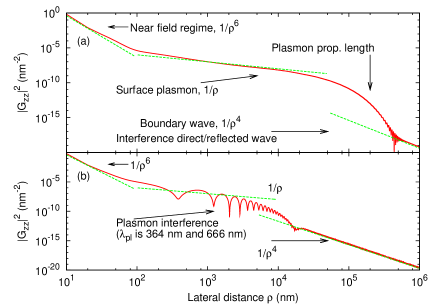
Figure 2: (color online) Behavior of the absolute square of the $zz$ element of the Green’s function along the surface of (a) a gold sample, (b) a 20 nm thick gold film. The photon energy is 1.8 eV.

Our results for the amplitude squared of the $zz$ element of the Green’s function are shown in Fig. 2 (which uses a logarithmic scale on both axis). This figure illustrates that the field generated by a point source near a metal film and propagating outwards along the surface basically displays three different regimes: At short range from the source the dipole field originating from the source (and its image) dominates completely giving rise to a large field that however drops off as $1/\rho^{6}$. After that follows a range of distances where plasmon propagation along the surface gives the dominant contribution to the Green’s function. The plasmons are cylindrical waves confined to the metal surface so their amplitudes decay as $1/\sqrt{\rho}$ in the absence of power losses. A Au film on a glass substrate supports two different plasmons, and in this case we see interference between them. Eventually, once we get to lateral distances between the source and field points corresponding to the plasmon propagation length the Green’s function drops exponentially due to losses in the metal film and we enter the domain where the main contribution comes from a boundary wave, also known as a Norton wave, Nikitin:PRL:10 propagating along the interface.

Naively one may expect $|G_{zz}|^{2}$ to decay as $1/\rho^{2}$ in the boundary wave regime, but in fact one finds a faster decay, $\sim 1/\rho^{4}$. Refs.  Aigouy:07, ; Leveque:07, ; Yang:Lalanne:09, ; Nikitin:PRL:10, present a number of derivations of this behavior. The basic physical reason behind the rapid decay is a destructive interference between the direct wave emerging from the source, and the wave reflected off the surface. As is easily seen from the expressions in Eq. (49), exactly at grazing incidence (where $p_{l}=0$) both of the Fresnel reflection coefficients $f^{s}$ and $f^{p}$ equal -1, which means that to lowest order the sum of incident and reflected wave vanishes. Away from grazing incidence the incident and reflected wave do not cancel exactly and what remains (with $|G_{zz}|^{2}\sim 1/\rho^{4}$) is the result of the interference between these contributions.

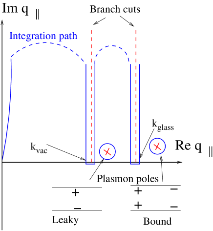
Figure 3: (color online) Deformation of the integration path in the complex plane in order to capture the asymptotic behavior of the Green’s function along the surface of the metal film.

In order to understand and calculate the asymptotic behavior of the Green’s function it is useful to study the behavior of the Fourier transform $\tensor{G}({q}_{\|},0,z,z^{\prime})$ in the complex plane. Figure 3 shows the general structure for the case of a three-layer structure vacuum/metal/dielectric. The FT has two branch points at $k_{B1}$ and $k_{B3}$, the vacuum and dielectric wave numbers. The physical branch cuts, as discussed in connection with Eq. (16), in this case follows the real axis back to the origin and then runs out along the positive imaginary axis. For the purpose of performing the Fourier integral for large separations between the source and field points it is, however, better to deform the branch cuts to run parallel with the imaginary as shown in Fig. 3.

Now the Bessel function in the integral Eq. (76) can be split into two Hankel functions as indicated in Eq. (78). The integral containing $H_{n}^{(2)}(q\rho)$ is calculated by deforming the contour to run far into the LHP, which for large $\rho$ yields negligible contributions. The integral containing $H_{n}^{(1)}(q\rho)$ is calculated by deforming the contour to run far into the UHP where this Hankel function is exponentially small so that the contributions from most of the contour are negligible. However, unlike in the LHP, the contour in the upper half plane must return to the real axis (or its vicinity) at every obstacle in the form of a branch cut or pole, and these parts of the integration path yield the dominating contributions to the Green’s function for large $\rho$. Miller:2006 The singularities closest to the real axis gives the contributions with the farthest range in $\rho$.

For the case illustrated in Figs. 2 and 3 the contributions from the integration along the branch cuts give the long-range, boundary wave contribution that persists over the entire range of distances in Fig. 2. A close look at the result for a film shows that the long-range tail exhibits some small oscillations between the contributions from the two different boundary waves, the one at the vacuum-gold interface and the one at the gold-glass interface.

As already said the boundary waves become the dominant contribution for values of $\rho$ beyond the plasmon propagation length. In Fig. 2(b) this happens around $\rho\sim 10\mathrm{\,\mu m}$. The behavior for $\rho\sim$ 1–10 $\mathrm{\,\mu m}$ is dictated by two different plasmons corresponding to the two poles in the UHP. The pole to the right of both branch cuts corresponds to a charge-symmetric, bound plasmon with a wavelength of 364 nm, shorter than the wavelengths of $\hbar\omega=1.8\mathrm{\,eV}$ light in both glass and vacuum. This mode is thus bound to the film, evanescent in both vacuum and glass, and the pole lies on the physical sheet of the Riemann surface. The other plasmon with a wavelength 666 nm is evanescent in vacuum, but propagating in glass. Therefore this charge-asymmetric mode is termed leaky since energy is lost to the glass side.Stegeman:1986 From a formal point of view this mode does not correspond to a bound state and the corresponding pole lies on a higher sheet of the Riemann surface, but is brought out in the open by the contour deformation.

V Solution of the scattering problem

The ultimate goal with the use of the Green’s function method is of course to solve electrodynamics problems in the form of Eq.  (12) generalized to the situation with a layered background,

$$\vec{E}(\vec{r})=\frac{\tensor{L}\cdot\vec{j}(\vec{r})}{i\omega\varepsilon_{0}\varepsilon_{B}(\vec{r})}-\frac{\Delta\varepsilon(\vec{r)}}{\varepsilon_{B}(\vec{r})}\tensor{L}\cdot\vec{E}(\vec{r})$$

$$+\int_{V_{j}-V_{\delta}}\tensor{G}(\vec{r},\vec{r}^{\prime})\left(i\omega\mu_{0}\vec{j}(\vec{r}^{\prime})+k_{0}^{2}\Delta\varepsilon(\vec{r^{\prime}})\vec{E}(\vec{r^{\prime}})\right)d^{3}r^{\prime}.$$

(98)

We focus on the case where the current sources $\vec{j}$ are well separated from the scatterers so that the contribution from the current term in the integral in Eq. (12) can be written as an incident field,

$$\vec{E}_{0}(\vec{r})=\int_{V_{j}-V_{\delta}}\tensor{G}(\vec{r},\vec{r}^{\prime})i\omega\mu_{0}\vec{j}(\vec{r}^{\prime})d^{3}r^{\prime}.$$ (99)

If the sources are very far away we have a situation where a plane wave is incident on the layered system, and gives rise to reflected and transmitted waves in the system, all of this is dictated by the presence of the Green’s function in Eq. (99). With an incident field written as $\vec{E}_{\mathrm{inc}}e^{i\vec{k}\cdot\vec{r}}$ we obtain a driving field $\vec{E}_{0}(\vec{r})$ in the layered system in accordance with Eq. (97).

Then Eq. (98) can be written

$$\vec{E}(\vec{r})=\vec{E}_{0}(\vec{r})-\frac{\Delta\varepsilon(\vec{r)}}{\varepsilon_{B}(\vec{r})}\tensor{L}\cdot\vec{E}(\vec{r})+\int_{V_{j}-V_{\delta}}\tensor{G}(\vec{r},\vec{r}^{\prime})k_{0}^{2}\Delta\varepsilon(\vec{r^{\prime}})\vec{E}(\vec{r^{\prime}})d^{3}r^{\prime}.$$ (100)

By moving all terms involving the full field $\vec{E}(\vec{r})$ to the left-hand side, thus leaving only the driving field $\vec{E}_{0}(\vec{r})$ on the right hand side, and then discretizing the electric field on a mesh of equally sized cubic elements that covers all scatterers we arrive at

$$\vec{E}_{qrs}+\frac{\Delta\varepsilon_{qrs}}{\varepsilon_{B,qrs}}\tensor{L}\cdot\vec{E}_{qrs}-k_{0}^{2}\Delta\varepsilon_{qrs}\tensor{M}\vec{E}_{qrs}-{\sum_{q^{\prime}r^{\prime}s^{\prime}}}^{{}^{\prime}}k_{0}^{2}\Delta\varepsilon_{q^{\prime}r^{\prime}s^{\prime}}V_{M}\tensor{G}_{q-q^{\prime},r-r^{\prime},s,s^{\prime}}\vec{E}_{q^{\prime}r^{\prime}s^{\prime}}=\vec{E}_{0,qrs}.$$ (101)

Here $q$, $r$, and $s$ are discrete coordinates for the mesh elements in the $x$, $y$, and $z$ directions, respectively. With a mesh side $a_{M}$ and an equivalent radius $R_{M}$ the volume of a mesh element is

$$V_{M}=a_{M}^{3}=\frac{4\pi R_{M}^{3}}{3}.$$ (102)

The term containing $\tensor{M}$ describes self interaction within a mesh element. We use an approximation for $\tensor{M}$ corresponding to a spherical mesh element of radius $R_{M}$,

$$\tensor{M}=\frac{2}{3k_{0}^{2}}\left[(1-ik_{0}R_{M})\exp(ik_{0}R_{M})-1\right]\tensor{1}.$$ (103)

At the same time the self-interaction term is excluded from the sum (as indicated by the prime) since including this would involve singular contributions to the Green’s function.

Equation (101) corresponds to a system of linear equations; the left hand side can be seen as a $3N_{M}\times 3N_{M}$ matrix multiplying a vector with $3N_{M}$ elements, $N_{M}$ being the total number of mesh elements. We solve the system of equations iteratively using the stabilized biconjugate gradient method, BiCGstab(2).Sleijpen:93 ; *Sleijpen:94 The iterative solution involves a large number of matrix multiplications. The contribution from the term in which the Green’s function multiplies the electric field is, as can be seen in Eq. (101), the result of a convolution sum in the $x$ and $y$ directions. This means that the matrix multiplication can be speeded up by using a Fast Fourier transform (FFT) in these two directions.Golub:1996 ; *NumRec The same technique is used in the DDA method.Draine:94 We calculate the Fourier transforms of the Green’s function and the electrical field and multiply the transforms by each other locally on the mesh in Fourier space and then transform the product back to the real space mesh. The use of the FFT is crucial in reducing computation times, since most of the computational effort required in determining the electric field in the scattering volume goes into solving the equation system, thus essentially the repeated matrix multiplications. The calculation of the Green’s function, on the other hand, just needs to be done once per photon frequency, combination of $z$ and $z^{\prime}$, and in-plane distance $\rho$.

Once we have a converged solution to the system of equations the electric field inside the scatterers is known. At this point Eq. (100) provides an explicit expression for the electric field everywhere else in space that can be evaluated by discretizing the integral as in Eq. (101).

The results presented in the next section focuses on the scattering cross section and thus depend on the far field which can be found from a discretized version of Eq. (90) using Eqs. (92) and (94). The scattering cross section is given by

$$\frac{d\sigma}{d\Omega}=\frac{r^{2}S_{r}}{S_{in}},$$ (104)

where $S_{r}$ is the radial component of the Poynting vector at a large distance $r$ from the scatterers and $S_{in}$ is the Poynting vector of the incident field. Given the (transverse) far field $\vec{E}(\vec{r})$,

$$S_{r}=\frac{1}{2}\,c\,\varepsilon_{0}\,\sqrt{\varepsilon_{B}}|\vec{E}(\vec{r})|^{2},$$ (105)

where $\varepsilon_{B}$ is the dielectric function of the material the radiation is scattered into.

VI Scattering off nanoholes in a thin metal film

We now turn to calculating scattering spectra off nanoholes in a thin Au film. Such systems have been studied experimentally by Rindzevicius et al.Tomas:hole:07 and Alaverdyan et al.Alaverdyan:hole:natphys:07

Figure 4: Illustration of illumination of two nanoholes with an electric field parallel to the dimer axis [in (a)], and perpendicular to the dimer axis [in (b)]. We also indicate how charges in the metal film surrounding the holes will be distributed in the case that the frequency of the incident light lies well below the single-hole resonance. One should note that the behavior of nanoholes in terms of induced charges is essentially opposite to that of metallic nanoparticles.

To study the problem theoretically we let a number of circular cylindrical holes in a Au film on top of a glass substrate act as scatterers. The Au film here has the same thickness, 20 nm, as in the experimental studies. The system is driven by a plane wave that impinges on the film (and the holes) at normal incidence, polarized either parallel to the symmetry axis of the hole chain or perpendicular to that symmetry axis, as illustrated in Fig. 4. We study primarily the forward scattering cross section as the edge-to-edge distance $d$, between the holes is varied.

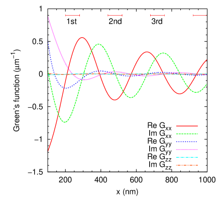
Figure 5: (color online) The diagonal components of the Green’s function as a function of the lateral distance $x$ along a 20 nm thick Au film on a glass substrate. Both the source and field points are placed in the middle of the film to best describe hole-hole interaction. The marks near the upper border show where the 1st, 2nd, and 3rd neighbor hole is placed in a chain of holes with a radius of 40 nm and edge-to-edge distance $d=160\mathrm{\,nm}$. (We stress, though, that the Green’s function here has been calculated in the absence of any holes.)

As a prelude we look at the Green’s function with both the source and field points placed inside the metal film, which is a central quantity determining the interaction between different nanoholes in the film. Figure 5 displays the behavior of the diagonal elements of $\tensor{G}$ for the vacuum/Au film/glass substrate system at a representative photon energy of 1.8 eV ($\lambda\approx 690\mathrm{\,nm}$) as a function of the lateral separation $x$. The $xx$ element is by far the strongest over most of the range of distances $x$, between the source and field points. A source pointing in the $x$ direction can excite plasmons propagating in the $x$ direction which explains why we have long-range interactions in this case. These plasmons are of the bound, charge-symmetric type discussed in Sec. IV, and illustrated in Fig. 3. The bound plasmon wavelength for $\hbar\omega=1.8\mathrm{\,eV}$ is $\approx 364\mathrm{\,nm}$. The $yy$ element is of comparable strength as $G_{xx}$ for distances up to $\sim 200\mathrm{\,nm}$, i.e. in the near-field zone. However, for larger $x$ the $yy$ element is much smaller because a dipole pointing in the $y$ direction cannot excite plasmons propagating in the $x$ direction. Finally looking at $G_{zz}$ we see that this component is much smaller than $G_{xx}$ for all $x$ values. This is due to the boundary conditions for the electric field at a metal interface, which strongly suppress the normal component inside the metal. As a consequence of reciprocity this also means that a source inside the metal film oriented perpendicular to the interfaces is not very effective in generating electric fields elsewhere.

Figure 6: (color online) Calculated forward scattering spectra for two nanoholes of diameter 80 nm in a 20 nm thick Au film placed on a glass substrate illuminated at normal incidence by light polarized parallel to the dimer axis. The different curves show results for a series of edge-to-edge distances $d$ between the holes as indicated in the key. The curve marked “1 hole” shows the corresponding result, adjusted for the scattering volume, for the case of a single hole.

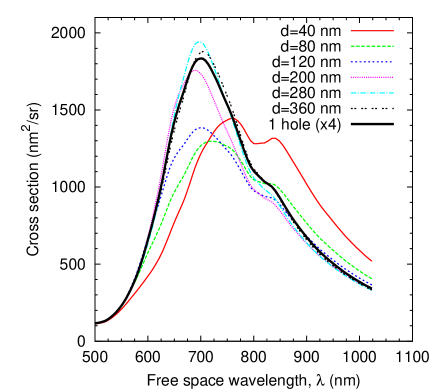
Figure 7: (color online) Forward scattering spectra for two nanoholes as in Fig. 6, however, here the incident light is polarized perpendicular to the dimer axis.

The behavior of different elements of the Green’s function leads to differences in the hole-hole interaction depending on the polarization direction of the incident light (illustrated in Fig. 4); interaction effects are much more important in the case of parallel polarization. The consequences are clearly seen in Figs. 6 and 7. Figure 6, to begin with, shows calculated scattering cross sections for two nanoholes of diameter 80 nm that are illuminated by light polarized parallel to the dimer axis. Each curve corresponds to a different edge-to-edge separation between the holes. To make a comparison that brings out the effect of hole-hole interactions the result for a single hole is also shown. This result is multiplied by 4 to adjust to the difference in scattering volume between the one- and two-hole cases. For a small separation between the holes the scattering cross section is suppressed and blue-shifted compared with the one-hole case. This is a result of $G_{xx}$ being negative for $x$ smaller than $\approx 200\mathrm{\,nm}$ (an edge-to-edge separation of 40 nm corresponds to a center-to-center distance of 120 nm). The shift can also be understood in view of Fig. 4(a): the figure shows that for frequencies below resonance the field caused by the induced charges at one hole will counteract the external field at the other hole, but this situation is reversed for frequencies above the single-hole resonance hence the blue-shift. With an increasing distance between the holes the scattering cross section increases and its maximum red-shifts, and a maximum in the cross section occurs for $d=160\mathrm{\,nm}$, corresponding to a distance of 240 nm between the hole centers. As can be seen in Fig. 5 this is close to the distance where $\mathrm{Re}[G_{xx}]$ has a maximum. In this situation there is a constructive interference at one hole between the incident field and the field scattered off the other hole. For larger $d$ the scattering cross section continues to red-shift, while the peak value falls off. For the largest separation $d=360\mathrm{\,nm}$, we in fact see a new peak building up at the blue end of the spectrum (near 650 nm). For even larger $d$ this peak grows and red-shifts reaching a second maximum around $d=560\mathrm{\,nm}$ corresponding to a center-to-center separation right near the second maximum of $\mathrm{Re}[G_{xx}]$ in Fig. 5 at $x\approx 650\mathrm{\,nm}$. In Ref. Alaverdyan:hole:natphys:07, it is argued that the scattering from a chain of holes should show maxima whenever an odd number of half surface plasmon wavelengths can be fit in between two holes. We note that in the present case with $\lambda_{\mathrm{pl}}=364\mathrm{\,nm}$, this predicts scattering maxima for $d=\lambda_{\mathrm{pl}}/2=182\mathrm{\,nm}$ and $d=3\lambda_{\mathrm{pl}}/2=546\mathrm{\,nm}$, which indeed agrees very well with the calculated results. Still, looking at the behavior of the Green’s function is a more general way of predicting resonance conditions.

The results in Fig. 7 calculated with the incident light polarized perpendicular to the hole dimer axis show much less variation with $d$. There is a suppression and a red-shift of the cross section for $d=40\mathrm{\,nm}$. This is expected given the basic behavior illustrated in Fig. 4(b) since in this case the field from the induced charges acts to enhance the external field at frequencies below the single-hole resonance. But with increasing $d$ the two-hole result rather quickly approaches the adjusted one-hole result, i.e. the spectrum is only marginally affected by hole-hole interactions. This can be anticipated by a look at the results for $G_{yy}$ in Fig. 5 which shows that the long-range interaction is rather weak for this configuration.

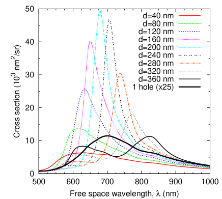
Figure 8: (color online) Forward scattering spectra for 5 nanoholes illuminated by light polarized along the axis of the chain of holes. The remaining parameters are the same as in Fig. 6.

Figures 8 and 9 show scattering spectra for chains of 5 and 8 holes, respectively, illuminated by light polarized along the axis of the chain. These results show the same trends as those in Fig. 6, but one can still make some additional observations. (i) The fact that we have more holes means that the collective effects of hole-hole interactions are stronger since the holes inside the chain now have two nearest neighbors. Consequently the peak position shifts more now when changing $d$ and the spectra rise higher above the (adjusted) one-hole result. (ii) The maximum scattering cross section is obtained at somewhat larger values of $d$ compared with the two-hole case. The reason is that not only nearest-neighbor interactions matter now. The cross section can be increased by moving the next-nearest neighbor hole closer to the second maximum of $\mathrm{Re[G_{xx}]}$ at $x=650\mathrm{\,nm}$, see Fig. 5, something that is achieved by an increase of $d$. (iii) We also see that the spectral features are sharper here than in the two-hole case. This is a rather natural consequence of the facts discussed above. An increasing number of holes brings an increasing degree of collective behavior and constructive interference to the optical response of the hole system, which at the same time is more sensitive to changes in either the photon energy of the incident light, the hole-hole separation, or for that matter the dielectric environment. Going from 2 holes to 5 makes more of a qualitative difference than increasing the number from 5 to 8. The reason for this is primarily the fact that nearest-neighbor interactions play a dominant role; with two holes in the chain both of them just have one nearest neighbor, whereas for 5- or 8-hole chains the majority of the holes have two nearest neighbors.

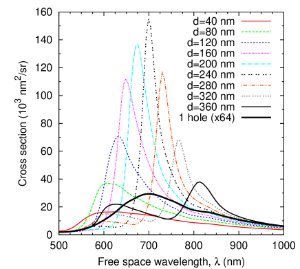
Figure 9: (color online) Forward scattering spectra for 8 nanoholes illuminated by light polarized along the axis of the chain of holes. The remaining parameters are the same as in Fig. 6.

The results presented here agree very well with the experimental results found in Ref. Alaverdyan:hole:natphys:07, , see in particular Fig. 2 there. (i) As in the experiment nanohole interactions play an important role when the electric field is polarized along the axis of the hole chain, while interactions only have a minor influence on the spectrum in the case of perpendicular polarization. (ii) For parallel polarization the experimental scattering spectrum goes through the same development as in Figs. 6, 8, and 9. For the smallest edge-to-edge distances the spectrum is suppressed and blue-shifted, but as $d$ increases a strong successively red-shifted peak builds up. (iii) The maximum scattering cross section in the two-hole case is reached for $d=160\mathrm{\,nm}$ here, and for $d=150\mathrm{\,nm}$ in the experiment, see Fig. 2(a) of Ref. Alaverdyan:hole:natphys:07, . These peak wavelengths differ somewhat, $\approx 655\mathrm{\,nm}$ in the experiment and $\approx 675\mathrm{\,nm}$ here, part of the reason for this is probably that the holes used in the experiment were somewhat smaller, with a diameter of 75 nm. (iv) Comparing the experimental results for 8 holes with those for 2 holes [Fig 2(a) of the experimental paper] we also see much the same trends as discussed above. More holes give stronger and sharper peaks and bigger wavelength shifts as a function of the edge-to-edge distance, just as in the calculation.

VII Summary

In this paper we have presented a derivation of the electromagnetic Green’s function in systems where the background dielectric function varies stepwise along one of the coordinate directions, $z$. The derivation is built on a transfer-matrix calculation of the Fourier transform of the GF. We have discussed certain symmetry properties of the Green’s function and also studied its long-range properties in real space based on the analytic properties of the Fourier transform in the complex plane.

As an example of an application we have studied the long-range properties of the Green’s function near a thin Au film on a glass substrate. We find there three different regimes depending on the lateral distance $\rho$ between the source and field points: (i) A near-field regime where the the square of the GF decay as $1/\rho^{6}$. (ii) For $100\mathrm{\,nm}\lesssim\rho\lesssim 10\mathrm{\,\mu m}$ the Green’s function is dominated by contributions from propagating surface plasmons, and $|G|^{2}\sim 1/\rho$. (iii) Finally, for larger distances, beyond the surface plasmon propagation length, the Green’s function is dominated by contributions from boundary waves (Norton waves) grazing the interface. A nearly destructive interference between the incident and reflected wave results in the intensity $\propto|G|^{2}$ decaying as $1/\rho^{4}$ in this case.

We have also applied the Green’s function method to a calculation of the scattering off two or several nanoholes in a thin Au film. We find a strong hole-hole interaction mediated by the surface plasmons of the Au film provided that the incident electric field is polarized along the axis of the hole chain. By increasing the number of holes the scattering spectrum gets sharper features and becomes more sensitive to changes in geometry, photon energy, or dielectric environment, something that can have applications in for example biochemical sensing.

References

- (1) W. L. Barnes, A. Dereux, and T. W. Ebbesen, Nature 424, 824 (2003)
- (2) J. K. Gimzewski, J. K. Sass, R. R. Schlitter, and J. Schott, Europhys. Lett. 8, 435 (1989)
- (3) R. Berndt, J. K. Gimzewski, and P. Johansson, Phys. Rev. Lett. 67, 3796 (1991)
- (4) X. H. Qiu, G. V. Nazin, and W. Ho, Science 299, 542 (2003)
- (5) Z.-C. Dong, X.-L. Guo, A. S. Trifonov, P. S. Dorozhkin, K. Miki, K. Kimura, S. Yokoyama, and S. Mashiko, Phys. Rev. Lett. 92, 086801 (2004)
- (6) N. L. Schneider, G. Schull, and R. Berndt, Phys. Rev. Lett. 105, 026601 (2010)
- (7) S. Nie and S. R. Emory, Science 275, 1102 (1997)
- (8) K. Kneipp, Y. Wang, H. Kneipp, L. T. Perelman, I. Itzkan, R. R. Dasari, and M. S. Feld, Phys. Rev. Lett. 78, 1667 (1997)
- (9) H. Xu, E. J. Bjerneld, M. Käll, and L. Börjesson, Phys. Rev. Lett. 83, 4357 (1999)
- (10) A. M. Michaels, M. Nirmal, and L. E. Brus, J. Am. Chem. Soc. 121, 9932 (1999)
- (11) T. W. Ebbesen, H. J. Lezec, H. F. Ghaemi, T. Thio, and P. A. Wolff, Nature 391, 667 (1998)
- (12) A. Dahlin, M. Zäch, T. Rindzevicius, M. Käll, D. S. Sutherland, and F. Höök, J. Am. Chem. Soc. 127, 5043 (2005)
- (13) P. C. Waterman, Phys. Rev. D 3, 825 (1971)
- (14) F. J. García de Abajo, Phys. Rev. B 59, 3095 (1999)
- (15) H.-X. Xu, Phys. Lett. A 312, 411 (2003)
- (16) P. Johansson, H. Xu, and M. Käll, Phys. Rev. B 72, 035427 (2005)
- (17) K. S. Yee, IEEE Trans. Antennas Propag. 14, 302 (1966)
- (18) C. T. Chan, Q. L. Yu, and K. M. Ho, Phys. Rev. B 51, 16635 (1995)
- (19) A. J. Ward and J. B. Pendry, Phys. Rev. B 58, 7252 (1998)
- (20) C. Oubre and P. Nordlander, J. Phys. Chem. B 108, 17740 (2004)
- (21) B. T. Draine and P. J. Flatau, J. Opt. Soc. Am. A 11, 1491 (1994)
- (22) E. M. Purcell and C. R. Pennypacker, Astrophys. J. 186, 705 (1973)
- (23) O. J. F. Martin, A. Dereux, and C. Girard, J. Opt. Soc. Am. A 11, 1073 (1994)
- (24) O. J. F. Martin, C. Girard, and A. Dereux, Phys. Rev. Lett. 74, 526 (1995)
- (25) M. Paulus, P. Gay-Balmaz, and O. J. F. Martin, Phys. Rev. E 62, 5797 (2000)
- (26) A. Y. Nikitin, G. Brucoli, F. J. García-Vidal, and L. Martín-Moreno, Phys. Rev. B 77, 195441 (2008)
- (27) J. Jung and T. Søndergaard, Phys. Rev. B 77, 245310 (2008)
- (28) E. Simsek, Opt. Expr. 18, 1722 (2010)
- (29) T. Rindzevicius, Y. Alaverdyan, B. Sepulveda, T. Pakizeh, M. Käll, R. Hillenbrand, J. Aizpurua, and F. J. Garcia de Abajo, J. Phys. Chem. C 111, 1207 (2007)
- (30) Y. Alaverdyan, B. Sepulveda, L. Eurenius, E. Olsson, and M. Käll, Nature Physics 3, 884 (2007)
- (31) F. J. G. de Abajo, Rev. Mod. Phys. 79, 1267 (2007)
- (32) T.-H. Park, N. Mirin, J. B. Lassiter, C. L. Nehl, N. J. Halas, and P. Nordlander, ACS Nano 2, 25 (2008)
- (33) B. Sepulveda, Y. Alaverdyan, J. Alegret, M. Käll, and P. Johansson, Opt. Expr. 16, 5609 (2008)
- (34) J. Alegret, P. Johansson, and M. Käll, New J. Phys. 10, 105004 (2008)
- (35) J. W. Lee, T. H. Park, P. Nordlander, and D. M. Mittleman, Phys. Rev. B 80, 205417 (2009)
- (36) E. J. R. Vesseur, F. J. Garćía de Abajo, and A. Polman, Nano Lett. 9, 3147 (2009)
- (37) J. A. Porto, F. J. García-Vidal, and J. B. Pendry, Phys. Rev. Lett. 83, 2845 (1999)
- (38) L. Martín-Moreno, F. J. García-Vidal, H. J. Lezec, K. M. Pellerin, T. Thio, J. B. Pendry, and T. W. Ebbesen, Phys. Rev. Lett. 86, 1114 (2001)
- (39) F. J. Garcia-Vidal, L. Martin-Moreno, T. W. Ebbesen, and L. Kuipers, Rev. Mod. Phys. 82, 729 (2010)
- (40) R. Gordon, A. G. Brolo, D. Sinton, and K. L. Kavanagh, Laser Photonics. Rev. 4, 311 (2010)
- (41) A. D. Yaghjian, Proc. IEEE 68, 248 (1980)
- (42) We define the homogeneous Green’s function to vanish identically, , whenever the source and field points are in different layers.
- (43) L. Aigouy, P. Lalanne, J. P. Hugonin, G. Julié, V. Mathet, and M. Mortier, Phys. Rev. Lett. 98, 153902 (2007)
- (44) G. Lévêque, O. J. F. Martin, and J. Weiner, Phys. Rev. B 76, 155418 (2007)
- (45) X. Y. Yang, H. T. Liu, and P. Lalanne, Phys. Rev. Lett. 102, 153903 (2009)
- (46) A. Y. Nikitin, F. J. García-Vidal, and L. Martín-Moreno, Phys. Rev. Lett. 105, 073902 (2010)
- (47) P. D. Miller, Applied Asymptotic Analysis, 1st ed. (American Mathematical Society, Providence, RI, 2006)
- (48) In this case, with different dielectric environments on each side of the metal film, the mode is of course not completely symmetric with respect to the surface charges.
- (49) J. J. Burke, G. I. Stegeman, and T. Tamir, Phys. Rev. B 33, 5186 (1986)
- (50) G. R. G. Sleijpen and D. R. Fokkema, Electron. Trans. Numer. Anal. 1, 11 (1993)
- (51) G. R. G. Sleijpen, H. A. van der Horst, and D. R. Fokkema, Numer. Algorithms 7, 75 (1994)
- (52) G. H. Golub and C. F. van Loan, Matrix Computations, 3rd ed. (The Johns Hopkins University Press, Baltimore, MD, 1996)
- (53) W. H. Press, B. P. Flannery, S. A. Teukolsky, and W. T. Vetterling, Numerical Recipes, 2nd ed. (Cambridge University Press, Cambridge, 1992)