Pricing and Hedging in Affine Models
with Possibility of Default

Abstract

We propose a general framework for the simultaneous modeling of equity, government bonds, corporate bonds and derivatives. Uncertainty is generated by a general affine Markov process. The setting allows for stochastic volatility, jumps, the possibility of default and correlation between different assets. We show how to calculate discounted complex moments by solving a coupled system of generalized Riccati equations. This yields an efficient method to compute prices of power payoffs. European calls and puts as well as binaries and asset-or-nothing options can be priced with the fast Fourier transform methods of Carr and Madan (1999) and Lee (2005). Other European payoffs can be approximated with a linear combination of government bonds, power payoffs and vanilla options. We show the results to be superior to using only government bonds and power payoffs or government bonds and vanilla options. We also give conditions for European continent claims in our framework to be replicable if enough financial instruments are liquidly tradable and study dynamic hedging strategies. As an example we discuss a Heston-type stochastic volatility model with possibility of default and stochastic interest rates.
Key words Pricing, hedging, affine models, stochastic volatility, jumps, default.

1 Introduction

The goal of this paper is to provide a flexible class of models for the consistent pricing and hedging of equity options, corporate bonds and government bonds. The noise in our models is driven by an underlying Markov process that can generate stochastic volatility, jumps and default. For the sake of tractability we assume it to be affine. Then discounted complex moments of the underlying can be calculated by solving a coupled system of generalized Riccati equations. This yields an efficient method to compute prices of power payoffs and the discounted characteristic function of the log stock price. From there, prices of vanilla options as well as binaries and asset-or-nothing options can be obtained with fast Fourier transform methods à la Carr and Madan [2] and Lee [15]. We also give conditions for European contingent claims in our models to be replicable if there exist enough liquid securities that can be used as hedging instruments.

Our framework can be seen as an extension of the unified pricing and hedging model of Carr and Schoutens [3], where market completeness is achieved through continuous trading in the money market, stock shares, variance swaps and credit default swaps. The authors suggest to approximate general payoffs with polynomials. In this paper we propose an approximations with a linear combination of government bonds, non-integer power payoffs and European calls.

Affine models have become popular in the finance literature because they offer a good trade-off between generality and tractability. One-factor affine processes were first used by Vasicek [22] and Cox–Ingersoll–Ross [4] for interest rates modeling. Popular affine stochastic volatility models include the ones by Stein and Stein [21] and Heston [9]. For affine models in credit risk we refer to Lando [13]. Here we work with general affine processes in the sense of Duffie et al. [6].

The rest of the paper is organized as follows. In Section 2 we introduce the model. In Section 3 we show how discounted complex moments can be calculated by solving generalized Riccati equations. This yields an efficient way of calculating options with power payoffs. As a corollary one obtains conditions for the discounted stock price to be a martingale under the pricing measure. The prices of vanilla options as well as binaries and asset-or-nothing options can be computed with the fast Fourier transform methods of Carr and Madan [2] and Lee [15]. For the pricing of European options with general payoffs we propose an $L^{2}$-approximation with a linear combination of government bonds, power payoffs and European calls. We illustrate this method by pricing a truncated log payoff, which can be applied to the valuation of a variance swap in the case where the underlying can default. Section 4 is devoted to the derivation of hedging rules. We show that in a model with discrete jumps, or no jumps at all, every European option can perfectly be hedged by trading in stock shares and a proper mix of European calls, government and corporate bonds. A system of linear equations is derived to find the hedging strategies. As an example we discuss in Section 5 a Heston-type stochastic volatility model with the possibility of default and stochastic interest rates.

2 The model

Let $(X_{t},\mathbb{P}_{x})_{t\geq 0,\;x\in D}$ be a time-homogeneous Markov process with values in $D:=\mathbb{R}^{m}_{+}\times\mathbb{R}^{n-m}$, $m\in\mathbb{N}$, $n\in\mathbb{N}\setminus\left\{0\right\}$. Let $\mathbb{E}_{x}$ be the expectation corresponding to $\mathbb{P}_{x}$ and denote by $\left\langle\cdot,\cdot\right\rangle$ the Euclidean (non-Hermitian) scalar product on $\mathbb{C}^{n}$: $\left<x,y\right>:=\sum_{i=1}^{n}x_{i}y_{i}$, $x,y\in\mathbb{C}^{n}$. Furthermore, set $\mathcal{I}=\{1,\dots,m\}$ and $\mathcal{J}=\{m+1,\dots,n\}$. $X_{{\cal I},t}$ and $X_{{\cal J},t}$ denote the first $m$ and last $n-m$ components of $X_{t}$, respectively.

We model the risk-neutral evolution of the price of a stock share by

$$S_{t}=\exp(s_{t}+R_{t}+\Lambda_{t})1_{\left\{t<\tau\right\}},$$

where

$$s_{t} = e+\left\langle\varepsilon,X_{t}\right\rangle\quad\mbox{for }(e,\varepsilon)\in\mathbb{R}\times\mathbb{R}^{n}$$

$$R_{t} = \int_{0}^{t}r_{u}du\quad\mbox{for }r_{t}=d+\left\langle\delta,X_{\mathcal{I},t}\right\rangle,\quad(d,\delta)\in\mathbb{R}_{+}\times\mathbb{R}^{m}_{+}$$

$$\Lambda_{t} = \int_{0}^{t}\lambda_{u}du\quad\mbox{for }\lambda_{t}=c+\left\langle\gamma,X_{\mathcal{I},t}\right\rangle,\quad(c,\gamma)\in\mathbb{R}_{+}\times\mathbb{R}^{m}_{+}$$

and

$$\tau=\inf\{t\geq 0:\Lambda_{t}=E\}$$

for a standard exponential random variable $E$ independent of $X$.

The process $r_{t}$ models the instantaneous risk-free interest rate and $\lambda_{t}$ the default rate. Note that both of them are non-negative. $\tau$ is the default time ($S_{t}=0$ for $t\geq\tau$), and $s_{t}$ describes the excess log-return of $S_{t}$ over $r_{t}+\lambda_{t}$ before default. Alternatively, one could model the three processes $\tilde{s}_{t}=s_{t}+R_{t}+\Lambda_{t}$, $R_{t}$ and $\Lambda_{t}$. But modeling $(s_{t},R_{t},\Lambda_{t})$ is convenient since it makes the discounted stock price equal to $\exp(s_{t}+\Lambda_{t})1_{\left\{t<\tau\right\}}$ and will allow us to give a simple condition for it to be a martingale under $\mathbb{P}_{x}$ (see Corollary 3.5 below).

For the sake of tractability we always assume that $(X_{t},\mathbb{P}_{x})_{t\geq 0,\;x\in D}$ is stochastically continuous and affine in the sense that
(H1) $X_{t}\to X_{t_{0}}$ in probability for $t\to t_{0}$ with respect to all $\mathbb{P}_{x}$, $x\in D$, and
(H2) there exist functions $\phi:\mathbb{R}_{+}\times i\mathbb{R}^{n}\to\mathbb{C}$ and $\psi:\mathbb{R}_{+}\times i\mathbb{R}^{n}\to\mathbb{C}^{n}$ such that

$$\mathbb{E}_{x}[\exp(\left\langle u,X_{t}\right\rangle)]=\exp\left(\phi(t,u)+\left\langle\psi(t,u),x\right\rangle\right)$$

for all $x\in D$ and $(t,u)\in\mathbb{R}_{+}\times i\mathbb{R}^{n}$.

It has been shown by Keller-Ressel et al. [12] that under the hypotheses (H1) and (H2), $(X_{t},\mathbb{P}_{x})_{t\geq 0,\;x\in D}$ automatically satisfies the regularity condition of Definition 2.5 in Duffie et al. [6]. Therefore, according to Theorem 2.7 in Duffie et al. [6], it is a Feller process whose infinitesimal generator ${\cal A}$ has $C^{2}_{c}(D)$ (the set of twice continuously differentiable functions $f:D\to\mathbb{R}$ with compact support) as a core and acts on $f\in C^{2}_{c}(D)$ like

$$\mathcal{A}f(x) = \sum_{k,l=1}^{n}\left(a_{kl}+\left<\alpha_{\mathcal{I},kl},x_{\mathcal{I}}\right>\right)\frac{\partial^{2}f(x)}{\partial x_{k}\partial x_{l}}+\left<b+\beta x,\nabla f(x)\right>$$

$$+\int_{D\backslash\{0\}}\left(f(x+\xi)-f(x)-\left<\nabla_{\mathcal{J}}f(x),\chi_{\mathcal{J}}(\xi)\right>\right)\nu(d\xi)$$

$$+\sum_{i=1}^{m}\int_{D\backslash\{0\}}\left(f(x+\xi)-f(x)-\left<\nabla_{\mathcal{J}\cup\{i\}}f(x),\chi_{\mathcal{J}\cup\{i\}}(\xi)\right>\right)x_{i}\mu_{i}(d\xi),$$

where $\chi=(\chi_{1},\dots,\chi_{n})$ for

$$\chi_{k}(\xi)=\begin{cases}0&\textrm{if $\xi_{k}=0$}\\ (1\wedge|\xi_{k}|)\frac{\xi_{k}}{|\xi_{k}|},&\textrm{otherwise}\end{cases}$$

and

• $a\in\mathbb{R}^{n\times n}$ is symmetric and positive semi-definite with $a_{\mathcal{II}}=0$

• $\alpha=(\alpha_{i})_{i\in\mathcal{I}}$, where for each $i\in\mathcal{I}$, $\alpha_{i}\in\mathbb{R}^{n\times n}$ is a positive semi-definite symmetric matrix such that all entries in $\alpha_{i,\mathcal{II}}$ are zero except for $\alpha_{i,ii}$

• $b\in D$

• $\beta\in\mathbb{R}^{n\times n}$ such that $\beta_{\mathcal{IJ}}=0$ and $\beta_{\mathcal{II}}$ has non-negative off-diagonal elements

• $\nu$ is a Borel measure on $D\backslash\{0\}$ with

  $$\int_{D\backslash\{0\}}\left(\left<\chi_{\mathcal{I}}(\xi),\mathbf{1}\right>+||\chi_{\mathcal{J}}(\xi)||^{2}\right)\nu(d\xi)<\infty$$

• $\mu=(\mu_{i})_{i\in\mathcal{I}}$ is a vector of Borel measures on $D\backslash\{0\}$ such that

  $$\int_{D\backslash\{0\}}\left(\left<\chi_{\mathcal{I}\backslash\{i\}}(\xi),\mathbf{1}\right>+||\chi_{\mathcal{J}\cup\{i\}}(\xi)||^{2}\right)\mu_{i}(d\xi)<\infty.$$

In addition we require the jumps to satisfy the following exponential integrability condition: For all $q\in\mathbb{R}^{n}$,

• $$\int_{D}e^{\left<q,\xi\right>}1_{\{||\xi||\geq 1\}}\nu(d\xi)<\infty\quad\mbox{and}\quad\int_{D}e^{\left<q,\xi\right>}1_{\{||\xi||\geq 1\}}\mu_{i}(d\xi)<\infty\quad\mbox{for all $i\in\mathcal{I}$}.$$

It follows from Theorem 2.7 and Lemma 9.2 in Duffie et al. [6] that for every set of parameters $(a,\alpha,b,\beta,\nu,\mu)$ satisfying (i)–(vii), (2) defines the infinitesimal generator of a $D$-valued Feller process $(X_{t},\mathbb{P}_{x})_{t\geq 0,\;x\in D}$ satisfying conditions (H1) and (H2) for $(\phi,\psi)$ equal to the unique solution of the following system of generalized Riccati equations

$$\begin{cases}\partial_{t}\phi(t,u)=F_{0}(\psi(t,u)),\quad\phi(0,u)=0\\ \partial_{t}\psi_{\mathcal{I}}(t,u)=F(\psi(t,u)),\quad\psi_{\mathcal{I}}(0,u)=u_{\mathcal{I}}\\ \psi_{\mathcal{J}}(t,u)=\exp(\beta^{T}_{\mathcal{JJ}}t)u_{\mathcal{J}}\end{cases},$$ (2.2)

where the functions $F_{0}:\mathbb{C}^{n}\to\mathbb{C}$ and $F:\mathbb{C}^{n}\to\mathbb{C}^{m}$ are given by

$$F_{0}(u) = \left<au,u\right>+\left<b,u\right>+\int_{D\backslash\{0\}}\left(e^{\left<u,\xi\right>}-1-\left<u_{\mathcal{J}},\chi_{\mathcal{J}}(\xi)\right>\right)\nu(d\xi)$$

$$F_{i}(u) = \left<\alpha_{i}u,u\right>+\sum_{k=1}^{n}\beta_{ki}u_{k}+\int_{D\backslash\{0\}}\left(e^{\left<u,\xi\right>}-1-\left<u_{\mathcal{J}\cup\{i\}},\chi_{\mathcal{J}\cup\{i\}}(\xi)\right>\right)\mu_{i}(d\xi),\quad i\in\mathcal{I}.$$

In particular, $(a,\alpha,b,\beta,\nu,\mu)$ uniquely determine the transition probabilities of $X$ and therefore, its distribution under each $\mathbb{P}_{x}$, $x\in D$. Since every Feller process has a RCLL version, we may assume $(X_{t},\tau,\mathbb{P}_{x})_{t\geq 0,x\in D}$ to be defined on ${\cal R}_{D}\times\mathbb{R}_{+}$, where ${\cal R}_{D}$ is the space of all RCLL functions $\omega:\mathbb{R}_{+}\to D$, and $(X_{t},\tau)(\omega,y)=(\omega(t),y)$.

3 Pricing

We price derivatives on $S_{t}$ by taking expectation under $\mathbb{P}_{x}$. For instance, we determine the price of a European option with payoff function $\varphi:\mathbb{R}_{+}\rightarrow\mathbb{R}$ and maturity $t>0$ by

$$\mathbb{E}_{x}\left[\exp\left(-R_{t}\right)\varphi(S_{t})\right].$$

Special cases include:

• Government bonds: $\varphi\equiv 1$

• Corporate bonds: $\varphi(x)=1_{\left\{x>0\right\}}$

• Call options: $\varphi(x)=(x-K)^{+}$ for $K>0$

• Power payoffs: $\varphi(x)=x^{p}1_{\{x>0\}}$ for $p\in\mathbb{R}$.

General power payoffs are not traded. But they can be priced efficiently and are helpful in pricing other payoffs. Moreover, for $p=1$, the price of the power payoff equals the stock price and having a general formula for $\mathbb{E}_{x}\left[\exp(-R_{t})S_{t}\right]$ will allow us to obtain conditions for the discounted stock price to be a martingale. The case $p=0$ corresponds to a corporate bond. We just consider zero coupon bonds and assume there is no recovery in the case of default. A corporate bond with a fixed recovery can be seen as a linear combination of a government and a corporate bond with no recovery. So all of the arguments that follow can easily be extended to this case.

In Subsection 3.1 we show how discounted moments of $S_{t}$ can be obtained by solving coupled systems of generalized Riccati equations. In Subsection 3.2 we extend Fourier pricing methods from Carr and Madan [2] and Lee [15] to our setup. In Subsection 3.3 we discuss the approximation of general European options with government bonds, power payoffs and European calls.

3.1 Discounted moments and generalized Riccati equations

For $t\geq 0$ and $x\in D$, define

$$U_{t,x}:=\left\{z\in\mathbb{C}:\mathbb{E}_{x}\left[\exp(-R_{t})S_{t}^{{\rm Re}(z)}1_{\{t<\tau\}}\right]<\infty\right\}$$

and the discounted moments function

$$h_{t,x}(z):=\mathbb{E}_{x}\left[\exp(-R_{t})S_{t}^{z}1_{\left\{t<\tau\right\}}\right],\quad z\in U_{t,x}.$$

Note that $U_{t,x}$ is equal to $\mathbb{C}$, a half-plane or a vertical strip. Since $R_{t}\geq 0$, it always contains the imaginary axis $i\mathbb{R}$. Clearly, $h_{t,x}$ is finite on $U_{t,x}$ and analytic in the interior of $U_{t,x}$. Indeed, $h_{t,x}(z)$ can be written as

$$h_{t,x}(z)=\mathbb{E}_{x}\left[\exp\left(zs_{t}+(z-1)R_{t}+z\Lambda_{t}\right)1_{\left\{t<\tau\right\}}\right].$$

So for $z$ in the interior of $U_{t,x}$, one can differentiate inside of the expectation to obtain

$$h^{\prime}_{t,x}(z)=\mathbb{E}_{x}\left[(s_{t}+R_{t}+\Lambda_{t})\exp\left(zs_{t}+(z-1)R_{t}+z\Lambda_{t}\right)1_{\left\{t<\tau\right\}}\right].$$

Let

$$A:\mathbb{R}_{+}\times\mathbb{C}^{n}\times\mathbb{C}\times\mathbb{C}\to\mathbb{C}\cup\left\{\infty\right\},\quad B:\mathbb{R}_{+}\times\mathbb{C}^{n}\times\mathbb{C}\times\mathbb{C}\to(\mathbb{C}\cup\left\{\infty\right\})^{n}$$

be solutions to the system of generalized Riccati equations

$$\begin{cases}\partial_{t}A(t,u,v,w)=G_{0}(B(t,u,v,w),v,w),\quad A(0,u,v,w)=0,\\ \partial_{t}B_{\mathcal{I}}(t,u,v,w)=G(B(t,u,v,w),v,w),\quad B_{\mathcal{I}}(0,u,v,w)=u_{\mathcal{I}},\\ B_{\mathcal{J}}(t,u,v,w)=\exp(\beta^{T}_{\mathcal{JJ}}t)u_{\mathcal{J}}\end{cases}$$ (3.1)

where the functions $G_{0}:\mathbb{C}^{n}\times\mathbb{C}\times\mathbb{C}\to\mathbb{C}$ and $G:\mathbb{C}^{n}\times\mathbb{C}\times\mathbb{C}\to\mathbb{C}^{m}$ are given by

$$G_{0}(u,v,w) = \left<au,u\right>+\left<b,u\right>+dv+c(w-1)+\int_{D\backslash\{0\}}\left(e^{\left<u,\xi\right>}-1-\left<u_{\mathcal{J}},\chi_{\mathcal{J}}(\xi)\right>\right)\nu(d\xi)$$

$$G_{i}(u,v,w) = \left<\alpha_{i}u,u\right>+\sum_{k=1}^{n}\beta_{ki}u_{k}+\delta_{i}v+\gamma_{i}(w-1)$$

$$+\int_{D\backslash\{0\}}\left(e^{\left<u,\xi\right>}-1-\left<u_{\mathcal{J}\cup\{i\}},\chi_{\mathcal{J}\cup\{i\}}(\xi)\right>\right)\mu_{i}(d\xi),\quad i\in\mathcal{I}.$$

The quadratic and exponential terms in $G_{i}$ can cause the solution $(A,B)$ of (3.1) to explode in finite time. However, since in condition (vii) we assumed the jumps of the process $X$ to have all exponential moments, we obtain from Lemma 5.3 of Duffie et al. [6] that the functions $G_{i}$, $i=0,\dots,m$, are analytic on $\mathbb{C}^{n+2}$. In particular, they are locally Lipschitz-continuous, and it follows from the Picard–Lindelöf Theorem that for every $(u,v,w)\in\mathbb{C}^{n}\times\mathbb{C}\times\mathbb{C}$ there exists $t^{*}>0$ such that equation (3.1) has a unique finite solution $(A,B)$ for $t\in[0,t^{*})$. We set $A$ and all components of $B$ equal to $\infty$ after the first explosion time. Note that the components $B_{j}(t,z\varepsilon,z-1,z)$, $j\in\mathcal{J}$, are finite and analytic in $z\in\mathbb{C}$ for all $t\geq 0$, and if $B_{i}(t,z\varepsilon,z-1,z)$ is finite/analytic in $z$ for all $i\in\mathcal{I}$, then so is $A(t,z\varepsilon,z-1,z)$. So for fixed $t\geq 0$, we define

$$V_{t}:=\{z\in\mathbb{C}:B_{i}(t,z\varepsilon,z-1,z)\mbox{ is finite for all }i\in\mathcal{I}\}.$$

and

$$l_{t,x}(z):=\exp\left\{ze+A(t,z\varepsilon,z-1,z)+\left<B(t,z\varepsilon,z-1,z),x\right>\right\},\quad z\in V_{t}.$$ (3.2)

In a first step we show the following

Lemma 3.1.

For every $t\geq 0$, $V_{t}$ contains $i\mathbb{R}$ and $h_{t,x}(z)=l_{t,x}(z)$ for all $x\in D$ and $z\in i\mathbb{R}$.

Proof.

Fix $\mathbb{P}_{x}$, $x_{n+1},x_{n+2}\in\mathbb{R}_{+}$ and denote $\hat{x}=(x,x_{n+1},x_{n+2})$. Consider the process

$$Y_{t}=\left\{\begin{array}[]{cl}(X_{t},x_{1}+R_{t},x_{2}+\Lambda_{t})&\textrm{for }t<\tau\\ \Delta&\textrm{for }t\geq\tau\end{array}\right.,$$

where $\Delta$ is a cemetery state outside of $\hat{D}:=\mathbb{R}_{+}^{m}\times\mathbb{R}^{n-m}\times\mathbb{R}^{2}_{+}$ to which $Y$ jumps at time $\tau$. $Y$ is a Markov process with values in $\hat{D}\cup\left\{\Delta\right\}$. Since $X$ has the properties (H1)–(H2), $Y$ fulfills the assumptions of Proposition III.2.4 of Revuz and Yor [19] and therefore is a Feller process. Moreover, $R_{t}=\int_{0}^{t}r_{u}du$ and $\Lambda_{t}=\int_{0}^{t}\lambda_{u}du$ are of finite variation and the random variable $E$ is independent of $X$. So one deduces from (H1) that for all $\hat{x}\in\hat{D}$ and $f\in C^{2}_{c}(\hat{D})$,

$$\frac{1}{t}\mathbb{E}_{x}[f(X_{t},x_{n+1}+R_{t},x_{n+2}+\Lambda_{t})1_{\left\{t<\tau\right\}}-f(x,x_{n+1},x_{n+2})]$$

$$= \frac{1}{t}\mathbb{E}_{x}\left[f(X_{t},x_{n+1},x_{n+2})-f(x,x_{n+1},x_{n+2})\right]$$

$$+\frac{1}{t}\mathbb{E}_{x}\left[f(X_{t},x_{n+1}+R_{t},x_{n+2}+\Lambda_{t})e^{-\Lambda_{t}}-f(X_{t},x_{n+1},x_{n+2})\right]$$

$$\to \hat{\cal A}f(\hat{x})\quad\mbox{for }t\downarrow 0,$$

where

$$\hat{\mathcal{A}}f(\hat{x}) = \sum_{k,l=1}^{n}\left(a_{kl}+\left<\alpha_{{\mathcal{I}},kl},x_{{\mathcal{I}}}\right>\right)\frac{\partial^{2}f(\hat{x})}{\partial x_{k}\partial x_{l}}+\left<\hat{b}+\hat{\beta}\hat{x},\nabla f(\hat{x})\right>-(c+\left<\gamma,x_{{\mathcal{I}}}\right>)f(\hat{x})$$

$$+\int_{D\setminus\{0\}}\left(f(\hat{x}+(\xi,0,0))-f(\hat{x})-\left<\nabla_{\mathcal{J}}f(\hat{x}),\chi_{\mathcal{J}}(\xi)\right>\right)\nu(d\xi)$$

$$+\sum_{i=1}^{m}\int_{D\backslash\{0\}}\left(f(\hat{x}+(\xi,0,0))-f(\hat{x})-\left<\nabla_{\mathcal{J}\cup\{i\}}f(\hat{x}),\chi_{\mathcal{J}\cup\{i\}}(\xi)\right>\right)x_{i}\mu_{i}(d\xi),$$

and

• $\hat{b}=(b,d,c)$

• $\hat{\beta}=\left(\begin{array}[]{cccc}\beta_{\mathcal{I}\mathcal{I}}&0&0&0\\ \beta_{\mathcal{J}\mathcal{I}}&\beta_{\mathcal{J}\mathcal{J}}&0&0\\ \delta&0&0&0\\ \gamma&0&0&0\end{array}\right)\in\mathbb{R}^{(n+2)\times(n+2)}$.

By Lemma 31.7 of Sato [20], the infinitesimal generator of $Y$ is well-defined and equal to $\hat{\cal A}$ on $C^{2}_{c}(\hat{D})$ (if $f(\Delta)$ is understood to be $0$ for $f\in C^{2}_{c}(\hat{D})$). But since $\hat{\cal A}$ is the infinitesimal generator of a regular affine process with values in $\hat{D}\cup\left\{\Delta\right\}$, it follows from Theorem 2.7 of Duffie et al. [6] that

$$\mathbb{E}_{x}\left[\exp\left(\left<u,X_{t}\right>+vR_{t}+w\Lambda_{t}\right)1_{\{t<\tau\}}\right]=\exp\left(A(t,u,v,w)+\left<B(t,u,v,w),x\right>\right).$$ (3.3)

for all $(t,u,v,w)\in\mathbb{R}_{+}\times\mathbb{C}_{-}^{m}\times(i\mathbb{R})^{n}\times\mathbb{C}_{-}^{2}$, where $\mathbb{C}_{-}$ denotes the set of all $z\in\mathbb{C}$ with $\mbox{Re}(z)\leq 0$. In particular, for $(t,u,v,w)\in\mathbb{R}_{+}\times\mathbb{C}_{-}^{m}\times(i\mathbb{R})^{n}\times\mathbb{C}_{-}^{2}$, $A(t,u,v,w)$ and all components of $B(t,u,v,w)$ are finite. In fact, according to Theorem 2.7 of Duffie et al. [6], the function $B$ should have $n+2$ components and $G$ should have $m+2$. But due to the special form of $\hat{\cal A}$, components $m+1$ and $m+2$ of $G$ vanish, and the corresponding components of $B$ stay equal to the initial values $v$ and $w$ for all times $t\geq 0$. In addition, $R_{0}=\Lambda_{0}=0$, and one obtains (3.3), where the functions $A$ and $B$ solve (3.1).

Now notice that

$$h_{t,x}(z)=\exp(ze)\mathbb{E}_{x}\left[\exp\left(z\left<\varepsilon,X_{t}\right>+(z-1)R_{t}+z\Lambda_{t}\right)1_{\{t<\tau\}}\right].$$

So, for all $t\geq 0$, $V_{t}$ contains $i\mathbb{R}$ and

$$h_{t,x}(z)=\exp\left\{ze+A(t,z\varepsilon,z-1,z)+\left<B(t,z\varepsilon,z-1,z),x\right>\right\}$$

for all $x\in D$ and $z\in i\mathbb{R}$. ∎

Lemma 3.2.

Fix $t_{0}\geq 0$ and $z_{0}\in V_{t_{0}}$. Then there exists an open neighborhood $W$ of $(t_{0},z_{0})$ in $\mathbb{R}_{+}\times\mathbb{C}$ such that

$$A(t,z\varepsilon,z-1,z)\quad\mbox{and}\quad B(t,z\varepsilon,z-1,z)$$

are finite for $(t,z)\in W$ as well as analytic in $t$ and $z$. In particular, the set

$$\left\{(t,z)\in\mathbb{R}_{+}\times\mathbb{C}:z\in V_{t}\right\}$$

is open and for all $x\in D$, $l_{t,x}(z)$ is analytic in $t$ and $z$.

Proof.

By Lemma 5.3 of Duffie et al. [6], the functions $G_{i}$, $i=0,\dots,m$, are analytic on $\mathbb{C}^{n+2}$. So, the lemma is a consequence of Theorem 1.1 in Ilyashenko and Yakovenko [10]. ∎

In the following theorem we extend the identity $h_{t,x}(z)=l_{t,x}(z)$ to $z$ outside of the imaginary axis $i\mathbb{R}$. Similar results in different settings have been given by Filipovic and Mayerhofer [8], Keller-Ressel [11], Spreij and Veerman [18].

Denote by $I_{t}$ the largest interval around $0$ contained in $V_{t}\cap\mathbb{R}$ and by $V^{0}_{t}$ the connected component of $V_{t}$ containing $0$. It follows from Lemma 3.2 that $I_{t}$ is open in $\mathbb{R}$, and it is clear that $I_{t}\subset V^{0}_{t}$. Moreover, one has

Theorem 3.3.

For all $(t,x)\in\mathbb{R}_{+}\times D$, $U_{t,x}$ is an open subset of $\mathbb{C}$ containing the strip $\left\{z\in\mathbb{C}:{\rm Re}(z)\in I_{t}\right\}$ and $h_{t,x}(z)=l_{t,x}(z)$ for each $z\in U_{t,x}\cap V^{0}_{t}$.

Proof.

For fixed $t\geq 0$ and $x\in D$, one can write

$$h_{t,x}(iy)=\mathbb{E}_{x}\left[\exp(-R_{t})1_{\left\{t<\tau\right\}}\right]\mathbb{E}_{\mathbb{Q}_{x}}\left[\exp(iy[s_{t}+R_{t}+\Lambda_{t}])\right],\quad y\in\mathbb{R},$$

where $\mathbb{Q}_{x}$ is the probability measure given by

$$\frac{d\mathbb{Q}_{x}}{d\mathbb{P}_{x}}=\frac{\exp(-R_{t})1_{\left\{t<\tau\right\}}}{\mathbb{E}_{x}\left[\exp(-R_{t})1_{\left\{t<\tau\right\}}\right]}.$$

So, up to a constant, $y\mapsto h_{t,x}(iy)$ is the characteristic function of $s_{t}+R_{t}+\Lambda_{t}$ with respect to $\mathbb{Q}_{x}$. From Lemmas 3.1 and 3.2 we know that $h_{t,x}(iy)=l_{t,x}(iy)$ for all $y\in\mathbb{R}$ and $V^{0}_{t}$ is an open neighborhood of $0$ in $\mathbb{C}$ on which $l_{t,x}$ is analytic. So it follows from Theorem 7.1.1 of Lukacs [16] that $U_{t,x}$ contains the strip $\left\{z\in\mathbb{C}:{\rm Re}(z)\in I_{t}\right\}$ and is open. Since $h_{t,x}(iy)=l_{t,x}(iy)$ for all $y\in\mathbb{R}$, $V^{0}_{t}$ is connected and both functions are analytic, one also has $h_{t,x}(z)=l_{t,x}(z)$ for $z\in U_{t,x}\cap V^{0}_{t}$. ∎

Remark 3.4.

The price of a corporate zero coupon bond with no recovery in the case of default is given by

$$P_{t,x}=\mathbb{E}_{x}\left[e^{-R_{t}}1_{\{S_{t}>0\}}\right]=h_{t,x}(0).$$

The price of a government bond is equal to the price of a corporate bond in a model where $(c,\gamma)=0$ (that is, the probability of default is zero).

Corollary 3.5.

The condition

$$G_{i}(\varepsilon,0,1)=0,\quad i=0,\dots,m,\quad\mbox{and}\quad\beta_{\mathcal{J}\mathcal{J}}=0,$$ (3.4)

is sufficient for the discounted stock price $\exp(s_{t}+\Lambda_{t})1_{\left\{t<\tau\right\}}$ to be a martingale with respect to all $\mathbb{P}_{x}$, $x\in D$. If all components of $\varepsilon_{\mathcal{J}}$ are different from $0$, then (3.4) is also necessary.

Proof.

It follows from Lemma 3.2 that there exists a $t_{0}>0$ such that $p\in V^{0}_{t}$ for all $(t,p)\in[0,t_{0}]\times[0,1]$. So if (3.4) holds, one obtains from Theorem 3.3 and (3.1) that

$$h_{t,x}(1)=\exp(e+A(t,\varepsilon,0,1)+\left<B(t,\varepsilon,0,1),x\right>)=h_{0,x}(1)\quad\mbox{for all }(t,x)\in[0,t_{0}]\times D.$$

Now the martingale property of $\exp(s_{t}+\Lambda_{t})1_{\left\{t<\tau\right\}}$ with respect to all $\mathbb{P}_{x}$, $x\in D$, follows by decomposing a given interval $[0,t]$ into finitely many intervals of length smaller than $t_{0}$ and taking iterative conditional expectations. If all components of $\varepsilon_{\mathcal{J}}$ are different from $0$ and condition (3.4) is violated, there exist $t\leq t_{0}$ and $x\in D$ such that $h_{t,x}(1)\neq h_{0,x}(1)$. So the martingale property cannot hold under $\mathbb{P}_{x}$. ∎

3.2 Pricing via Fourier transform

In this subsection we show how to extend Fourier pricing methods from Carr and Madan [2] and Lee [15] to our setting. Since $\mathbb{P}_{x}$ is used as pricing measure, one would typically work with models in which the discounted stock price $\exp(s_{t}+\Lambda_{t})1_{\left\{t<\tau\right\}}$ is a martingale under $\mathbb{P}_{x}$. However, the following results just involve $S_{t}$ for fixed $t\geq 0$ and technically do not need the discounted stock price to be a martingale.

Consider a call option with log strike $k$ and price

$$c_{t,x}(k)=\mathbb{E}_{x}\left[e^{-R_{t}}\left(S_{t}-e^{k}\right)^{+}\right].$$

Theorem 3.6.

Let $(t,x)\in\mathbb{R}_{+}\times D$ and $p>0$ such that $p+1\in U_{t,x}$. Then

$$c_{t,x}(k)=\frac{e^{-pk}}{2\pi}\int_{\mathbb{R}}e^{-iyk}g_{c}(y)dy=\frac{e^{-pk}}{\pi}\int_{0}^{\infty}{\rm Re}\left(e^{-iyk}g_{c}(y)\right)dy,$$ (3.5)

where

$$g_{c}(y)=\frac{h_{t,x}(p+1+iy)}{p^{2}+p-y^{2}+iy(2p+1)}.$$

Proof.

Since $U_{t,x}$ is open, there exists $\eta>0$ such that $p+1+\eta\in U_{t,x}$, and it follows from Corollary 2.2 in Lee [14] that

$$c_{t,x}(k)=O(e^{-(p+\eta)k})\quad\mbox{for }k\to\infty.$$

In particular,

$$\int_{\mathbb{R}}\left(e^{pk}c_{t,x}(k)\right)^{2}dk<\infty.$$

It follows that the Fourier transform

$$g_{c}(y)=\int_{\mathbb{R}}e^{iyk}e^{pk}c_{t,x}(k)dk$$

is square-integrable in $y$, and one can transform back to obtain

$$e^{pk}c_{t,x}(k)=\frac{1}{2\pi}\int_{\mathbb{R}}e^{-iyk}g_{c}(y)dy.$$

This shows the first equality of (3.5). Since $c_{t,x}(k)$ is real-valued, one has $g_{c}(-y)=\overline{g_{c}(y)}$, which implies the second inequality of (3.5). To conclude the proof, set $z=p+iy$ and note that

$$g_{c}(y) = \int_{\mathbb{R}}e^{zk}\mathbb{E}_{x}\left[\left(e^{s_{t}+\Lambda_{t}}-e^{k-R_{t}}\right)1_{\left\{s_{t}+R_{t}+\Lambda_{t}\geq k,\;t<\tau\right\}}\right]dk$$

$$= \mathbb{E}_{x}\left[\int_{-\infty}^{s_{t}+R_{t}+\Lambda_{t}}\left(e^{zk+s_{t}+\Lambda_{t}}-e^{(z+1)k-R_{t}}\right)dk1_{\left\{t<\tau\right\}}\right]$$

$$= \frac{1}{z(z+1)}\mathbb{E}_{x}\left[\exp(-R_{t}+(z+1)\log S_{t})1_{\left\{t<\tau\right\}}\right]$$

$$= \frac{1}{z(z+1)}h_{t,x}(z+1).$$

∎

To calculate prices of options with short maturities or extreme out-of-the money strikes Carr and Madan [2] suggest an alternative method which does not suffer from high oscillations. To adapt it to our setup, define

$$d_{t,x}(k):=\begin{cases}\mathbb{E}_{x}\left[e^{-R_{t}}\left(e^{k}-S_{t}\right)^{+}1_{\{t<\tau\}}\right]&\textrm{if }k<\log S_{0}\\ \\ \mathbb{E}_{x}\left[e^{-R_{t}}\left(S_{t}-e^{k}\right)^{+}\right]&\textrm{if }k>\log S_{0}\end{cases}.$$

Then the following holds:

Theorem 3.7.

Let $(t,x)\in\mathbb{R}_{+}\times D$ and $p>0$ such that $1-p,\;1+p\in U_{t,x}$. Then

$$d_{t,x}(k)=\frac{1}{\sinh(pk)}\frac{1}{2\pi}\int_{\mathbb{R}}e^{-iyk}g_{d}(y)dy,$$ (3.6)

where

$$g_{d}(y)=\frac{f(y-ip)-f(y+ip)}{2}$$

and

$$f(y)=\frac{\exp((1+iy)s_{0})}{1+iy}h_{t,x}(0)-\frac{\exp(iys_{0})}{iy}h_{t,x}(1)-\frac{h_{t,x}(1+iy)}{y^{2}-iy}.$$

Proof.

Since $U_{t,x}$ is open, there exists $\eta>0$ such that $1-p-\eta$ and $1+p+\eta$ belong to $U_{t,x}$. By Corollary 2.2 of Lee [14],

$$d_{t,x}(k)=O(e^{-(p+\eta)|k|})\quad\mbox{for }k\to\pm\infty.$$

In particular, $d_{t,x}(k)$ and $\sinh(pk)d_{t,x}(k)$ are both square-integrable in $k$. One easily checks that

$$\int_{\mathbb{R}}e^{iyk}d_{t,x}(k)dk=f(y).$$

So,

$$\int_{\mathbb{R}}e^{iyk}\sinh(pk)d_{t,x}(k)dk=\int_{\mathbb{R}}e^{iyk}\frac{e^{pk}-e^{-pk}}{2}d_{t,x}(k)dk\\ =\frac{f(y-ip)-f(y+ip)}{2},$$

and hence,

$$d_{t,x}(k)=\frac{1}{\sinh(pk)}\frac{1}{2\pi}\int_{\mathbb{R}}e^{-iyk}g_{d}(y)dy.$$

∎

There exist several extensions of the Fourier pricing methods of Carr and Madan [2]. For example, Lee [15] shows that (3.5) can be adjusted in order to allow for $p<0$ and derives pricing formulas for other European derivatives, such as binary or asset-or-nothing options. By adjusting the proof of Theorem 5.1 of [15] to our setup, one obtains the following: Denote

$$a_{t,x}(k)=\mathbb{E}_{x}\left[e^{-R_{t}}S_{t}1_{\{\log S_{t}>k\}}\right]\quad\mbox{and}\quad b_{t,x}(k)=\mathbb{E}_{x}\left[e^{-R_{t}}1_{\{\log S_{t}>k\}}\right].$$

Then

$$c_{t,x}(k)=a_{t,x}(k)-e^{k}b_{t,x}(k),$$

and one has

Theorem 3.8.

Let $(t,x)\in\mathbb{R}_{+}\times D$ and $p,\;q\in\mathbb{R}$ such that $p+1,\;q\in U_{t,x}$. Then

$$a_{t,x}(k)=R_{a}(p)+\frac{e^{-pk}}{\pi}\int_{0}^{\infty}{\rm Re}\left(e^{-iyk}g_{a}(y)\right)dy$$

$$b_{t,x}(k)=R_{b}(q)+\frac{e^{-qk}}{\pi}\int_{0}^{\infty}{\rm Re}\left(e^{-iyk}g_{b}(y)\right)dy$$

$$c_{t,x}(k)=R_{c}(p)+\frac{e^{-pk}}{\pi}\int_{0}^{\infty}{\rm Re}\left(e^{-iyk}g_{c}(y)\right)dy,$$

where

$$g_{a}(y)=-\frac{h_{t,x}(p+1+iy)}{p+iy},\quad g_{b}(y)=\frac{h_{t,x}(q+iy)}{q+iy},\quad g_{c}(y)=\frac{h_{t,x}(p+1+iy)}{p^{2}+p-y^{2}+iy(2p+1)}$$

and

$$R_{a}(p)=\begin{cases}h_{t,x}(1)&\textrm{if }p<0\\ \frac{h_{t,x}(1)}{2}&\textrm{if }p=0\\ 0&\textrm{if }p>0\end{cases},\quad R_{b}(q)=\begin{cases}h_{t,x}(0)&\textrm{if }q<0\\ \frac{h_{t,x}(0)}{2}&\textrm{if }q=0\\ 0&\textrm{if }q>0\end{cases}$$

$$R_{c}(p)=\begin{cases}h_{t,x}(1)-e^{k}h_{t,x}(0)&\textrm{if }p<-1\\ h_{t,x}(1)-\frac{e^{k}h_{t,x}(0)}{2}&\textrm{if }p=-1\\ h_{t,x}(1)&\textrm{if }-1<p<0\\ \frac{h_{t,x}(1)}{2}&\textrm{if }p=0\\ 0&\textrm{if }p>0\\ \end{cases}.$$

3.3 Approximation of general payoffs

3.3.1 Idea

The prices of European options with payoff functions in the set

$$L_{t,x}:=\left\{\varphi:\mathbb{R}_{+}\rightarrow\mathbb{R}\;\;\textrm{Borel-measurable such that }\mathbb{E}_{x}\left[e^{-R_{t}}|\varphi(S_{t})|\right]<\infty\right\}$$

can be approximated by portfolios consisting of securities that can either be priced directly or with Fourier methods. For most purposes it is sufficient to use a mix of $\varphi(0)$ government bonds, power payoffs and call options. For instance, let $p_{1}<\dots<p_{f}$ be a set of powers and $K_{1}<\dots<K_{g}$ finitely many strike prices. Then fix $s^{*}>0$ and determine weights $v_{1},\dots,v_{f}$ and $w_{1},\dots,w_{g}$ by weighted $L^{2}$-regression:

$$\mathop{\rm arg\,min}_{v,w}\int_{0}^{s^{*}}\left(\varphi(s)-\varphi(0)-\sum_{i=1}^{f}v_{i}s^{p_{i}}1_{\left\{s>0\right\}}-\sum_{i=1}^{g}w_{i}(s-K_{i})^{+}\right)^{2}\rho(s)ds,$$ (3.7)

where $\rho$ is a heuristic density approximation of $S_{t}$. The positive function $\rho$ is meant to put additional weight on regions where $S_{t}$ is more likely to lie (usually in the vicinity of $\mathbb{E}_{x}\left[S_{t}\right]$ and if default is possible, around $0$). If one does not have a good idea of the distribution of $S_{t}$, one can also use non-weighted regression ($\rho\equiv 1$).

If the integral is discretized, the optimization problem (3.7) becomes a finite-dimensional $L^{2}$-regression. To improve the numerical stability, one can first apply Gram–Schmidt orthogonalization to the basis functions $\varphi(0)$, $s^{p_{i}}1_{\left\{s>0\right\}}$ and $(s-K_{i})^{+}$.

3.3.2 Example: Truncated log payoff

We illustrate this method by approximating the price of a truncated log payoff $\varphi(s)=\log(s)\vee k$, $k\in\mathbb{R}$. Note that since $S_{t}=0$ with positive probability, the truncation from below is crucial.

Assume $S_{0}=1$ and $k=-1$. We consider three ways of approximating $\varphi$ with linear combinations of 101 instruments:

1. A government bond and power payoffs of powers $0.05,\;0.1,\dots,5$

2. A government bond and call options with strikes $0.03,\;0.06,\;\dots,3$

3. A government bond, power payoffs of powers $0.1,\;0.2,\dots,5$ and call options with strikes $0.06,\dots,3$

We let $s^{*}=3$. As heuristic density for $S_{t}$ we use $\rho$ given by

$$\rho(x)=\begin{cases}\exp(-10x)&x<0.5\\ \exp(-10|x-1|)&0.5\leq x\leq 1.5\\ \exp(-5)&x>1.5\end{cases}.$$ (3.8)

This choice of $\rho$ assigns more weight to $0$ and points around $1$. But it is just an example of what one could choose. Depending on the model and the value of $t$ one may want to use different functions $\rho$.

Figure 1 shows the errors of the three approximation methods. It can be seen that for the truncated log payoff methods 2 and 3 give a much better approximation than method 1. The errors of methods 2 and 3 are similar. But since prices of power payoffs are easier to calculate than those of call options, method 3 is significantly faster.

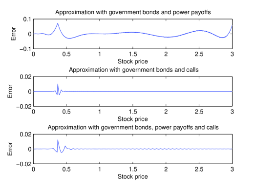
Figure 1: Comparison of different approximation methods. Note that the scales are different!

Log payoffs are useful in the pricing and hedging of variance swaps on futures. Let $F_{u}$, $0\leq u\leq t$, be the price of a futures contract on $S_{t}$ and consider a variance swap with time-$t$ cash-flow

$$\Sigma_{t}=\max\left(\frac{1}{t}\sum_{i=1}^{I}\left(\log\frac{F_{t_{i}}}{F_{t_{i-1}}}\right)^{2}-K,C\right),$$

where $0=t_{0}<\dots<t_{I}=t$ are the discrete monitoring points (usually daily), $K$ is the strike and $C$ is a cap on the payoff (typically $C=2.5K$). If $F_{u}$ is modeled as a positive continuous martingale of the form $dF_{u}=\sigma_{u}F_{u}dW_{u}$, then the probability of hitting the cap $C$ is negligible and one can approximate the sum with an integral:

$$\Sigma_{t}\approx\frac{1}{t}\int_{0}^{t}\sigma^{2}_{u}du-K.$$

It has been noticed by Dupire [5] and Neuberger [17] that

$$\int_{0}^{t}\sigma^{2}_{u}du=2\left(\int_{0}^{t}\frac{1}{F_{u}}dF_{u}-\log S_{t}+\log F_{0}\right),$$

and therefore,

$$\mathbb{E}_{x}\left[\frac{1}{t}\int_{0}^{t}\sigma^{2}_{u}du\right]=\frac{2}{t}\mathbb{E}_{x}\left[\log F_{0}-\log S_{t}\right].$$

In a diffusion model with the possibility of default the cap is crucial since it is hit in case of default. If one neglects the probability that the cap is hit before default or that $\log S_{t}<k:=\log(F_{0})-t(C+K)/2$ if there is no default, one can approximate $\Sigma_{t}$ as follows:

$$\Sigma_{t} \approx 1_{\left\{\tau>t\right\}}\left(\frac{1}{t}\int_{0}^{t}\sigma^{2}_{u}du-K\right)+1_{\left\{\tau\leq t\right\}}C$$

$$\approx \frac{2}{t}\left(\int_{0}^{t\wedge\tau}\frac{1}{F_{u-}}dF_{u}-(\log(S_{t})\vee k)+\log F_{0}\right)-K-1_{\left\{\tau\leq t\right\}}\frac{2}{t}\int_{0}^{\tau}\frac{1}{F_{u-}}dF_{u}.$$

In the special case where the default intensity is constant, the expectation of the last integral is zero, and one can price according to

$$\mathbb{E}_{x}\left[\Sigma_{t}\right]\approx\frac{2}{t}\mathbb{E}_{x}\left[\log F_{0}-\log(S_{t}\vee k)\right]-K.$$

4 Hedging

In this section we consider a subclass of affine models in which European contingent claims can perfectly be hedged by dynamically trading in sufficiently many liquid securities. Assume that condition (3.4) is fulfilled. So that the discounted stock price $\exp(s_{t}+\Lambda_{t})1_{\left\{t<\tau\right\}}$ is a martingale under all $\mathbb{P}_{x}$, $x\in D$. It is well-known that it is impossible to replicate contingents claims with finitely many hedging instruments in a model where the underlying has jumps of infinitely many different sizes. Therefore, we here require the jump measures $\nu$ and $\mu_{i}$, $i\in{\cal I}$, to be of the following form:

$$\nu = \sum_{q=1}^{M}v_{q}\delta_{y_{q}}\mbox{ for }v_{q}>0\mbox{ and different points }y_{1},\dots,y_{M}\mbox{ in }\in D\backslash\{0\}$$ (4.1)

$$\mu_{i} = \sum_{q=1}^{M_{i}}v_{iq}\delta_{y_{iq}}\mbox{ for }v_{iq}>0\mbox{ and different points }y_{i1},\dots,y_{iM_{i}}\mbox{ in }\in D\backslash\{0\},$$ (4.2)

where $\delta_{y_{q}}$, $\delta_{y_{iq}}$ are Dirac measures and for $M=0$ or $M_{i}=0$, $\nu$ or $\mu_{i}$ are understood to be zero, respectively. The integrability condition (vii) is then trivially satisfied.

In the following theorem we are going to show that the process $X$ has a realization as the unique strong solution of an SDE of the from

$$dX_{t}=\tilde{b}(X_{t})dt+\sigma(X_{t})dW_{t}+\int_{\mathbb{R}_{+}}k(X_{t-},z)N(dt,dz),$$ (4.3)

where $W$ is an $n$-dimensional Brownian motion and $N$ an independent Poisson random measure on $\mathbb{R}^{2}_{+}$ with Lebesgue measure as intensity measure. $\sigma:D\to\mathbb{R}^{n\times n}$ has to be a measurable function satisfying

$$\sigma\sigma^{T}(x)=a+\sum_{i\in{\cal I}}x_{i}\alpha_{i}\quad\mbox{for all $x\in D,$}$$ (4.4)

and the functions $\tilde{b}:D\to\mathbb{R}^{n}$ and $k:D\times\mathbb{R}_{+}\to D$ are of the following form:

$$\tilde{b}(x)=b+\beta x-\int_{D\setminus\left\{0\right\}}\chi_{\cal J}(\xi)\nu(d\xi)-\sum_{i=1}^{m}x_{i}\int_{D\setminus\left\{0\right\}}\chi_{{\cal J}\cup\left\{i\right\}}(\xi)\mu_{i}(d\xi),$$

$$k(x,z)=\left\{\begin{array}[]{ll}y_{q}&\mbox{ if }V_{q-1}\leq z<V_{q}\\ y_{iq}&\mbox{ if }V_{M}+\sum_{j=1}^{i-1}x_{j}V_{jM_{j}}+x_{i}V_{i(q-1)}\leq z<V_{M}+\sum_{j=1}^{i-1}x_{j}V_{jM_{j}}+x_{i}V_{iq}\\ 0&\mbox{ if }z\geq V_{M}+\sum_{j=1}^{m}x_{j}V_{jM_{j}}\end{array}\right.,$$

where $V_{q}=\sum_{p=1}^{q}v_{p}$ and $V_{iq}=\sum_{p=1}^{q}v_{ip}$. Theorem 4.1 is an extension of Theorem 8.1 in Filipovic and Mayerhofer [8]. Its proof is given in the appendix.

Theorem 4.1.

If $\nu$ and $\mu_{i}$, $i\in{\cal I}$, are of the form (4.1)–(4.2), then there exists a measurable function $\sigma:D\to\mathbb{R}^{n\times n}$ satisfying (4.4) such that the SDE (4.3) has for all initial conditions $x\in D$ a unique strong solution. It is Feller process satisfying (H1)–(H2) corresponding to the parameters $(a,\alpha,b,\beta,m,\mu)$.

In general, one needs $L+1:=n+M+\sum_{i=1}^{m}M_{i}+2$ instruments to hedge all sources of risk. We assume the first one to be a money market account yielding an instantaneous return of $r_{t}$. In addition, one needs one instrument for each of the $n$ components of the Brownian motion $W$, one for each of the possible jumps of $X$ and one for the jump to default (without default, $L$ instruments are generally enough). Of course, if the hedging instruments are redundant, not all European contingent claims can be replicated; precise conditions for a given option to be replicable are given in (4.5) below. The hedging instruments should also be liquidly traded. For instance, in addition to the money market account, one could use a mix of instruments of the following types:

• Stock shares

• Government bonds

• Corporate bonds

• Vanilla options.

All of these can be viewed as European options with different payoff functions. Let us denote the set of hedging instruments different from the money market account by

$$\Phi=\{(t_{1},\varphi_{1}),\dots,(t_{L},\varphi_{L})\},$$

where $t_{1},\dots,t_{L}$ are the maturities and $\varphi_{l}\in L_{t_{l},x}$ the payoff functions.

Now consider a European option with maturity $t\leq\min\left\{t_{1},\dots,t_{L}\right\}$ and payoff function $\varphi\in L_{t,x}$. At time $0$, its price is

$$\pi(t,x):=\mathbb{E}_{x}\left[\exp(-R_{t})\varphi(S_{t})\right],$$

and for $u\in[0,t]$,

$$C_{u}=\left\{\begin{array}[]{cl}\pi(t-u,X_{u})&\mbox{ if }u<\tau\\ \mathbb{E}_{x}\left[e^{-(R_{t}-R_{u})}\mid X_{u}\right]\varphi(0)&\mbox{ if }u\geq\tau\end{array}\right..$$

After the default time $\tau$, $C_{u}$ behaves like a government bond and can be hedged accordingly. To design the hedge before time $\tau$, we introduce the following sensitivity parameters:

• Classical Greeks: for $q=1,\dots,n$:

  $$H^{q}_{t,x}=\frac{\partial}{\partial x_{q}}\pi(t,x)$$

• Sensitivities to the jumps corresponding to $\nu$: for all $q=1,\dots,M$:

  $$J^{q}_{t,x}=\pi(t,x+y_{q})-\pi(t,x)$$

• Sensitivities to the jumps corresponding to $\mu$: for all $i\in\mathcal{I}$ and $q=1,\dots,M_{i}$:

  $$J^{iq}_{t,x}=\pi(t,x+y_{iq})-\pi(t,x)$$

• Sensitivity to default:

  $$D_{t,x}=\mathbb{E}_{x}\left[\exp(-R_{t})\varphi(0)\right]-\mathbb{E}_{x}\left[\exp(-R_{t})\varphi(S_{t})\right].$$

Example 4.2.

Consider a power payoff $\varphi(s)=s^{p}$ for some $p>0$ such that $s^{p}\in L_{t,x}$. Then the sensitivity parameters are given by

$$H^{q}_{t,x} = \frac{\partial}{\partial x_{q}}h_{t,x}(p)=B_{q}(t,p\varepsilon,p-1,p)h_{t,x}(p)$$

$$J^{q}_{t,x} = h_{t,x+y_{q}}(p)-h_{t,x}(p)$$

$$J^{iq}_{t,x} = h_{t,x+y_{iq}}(p)-h_{t,x}(p)$$

$$D_{t,x} = -h_{t,x}(p).$$

Example 4.3.

For a European call option with log strike $k$ and maturity $t$, the classical Greeks are

$$H^{q}_{t,x}=\frac{\partial}{\partial x_{q}}c_{t,x}(k)=\frac{e^{-pk}}{\pi}\int_{0}^{\infty}{\rm Re}\left(e^{-iyk}\partial_{x_{q}}g_{c}(y)\right)dy,$$

where

$$\partial_{x_{q}}g_{c}(y) = \partial_{x_{q}}\frac{h_{t,x}(p+1+iy)}{p^{2}+p-y^{2}+iy(2p+1)}$$

$$= \frac{B_{q}(t,(p+1+iy)\varepsilon,p+iy,p+1+iy)h_{t,x}(p+1+iy)}{p^{2}+p-y^{2}+iy(2p+1)}$$

for some $p>0$ such that $1+p\in U_{t,x}$. The other sensitivities are

$$J^{q}_{t,x} = c_{t,x+y_{q}}(k)-c_{t,x}(k)$$

$$J^{iq}_{t,x} = c_{t,x+y_{iq}}(k)-c_{t,x}(k)$$

$$D_{t,x} = -c_{t,x}(k).$$

As shown in Examples 4.2 and 4.3, the sensitivity parameters of power payoffs and vanilla options can be given in closed or almost closed form. The payoff $\varphi\in L_{t,x}$ can be approximated with a linear combination of government bonds, power payoffs and European calls of maturity $t$ as in Subsection 3.3. The sensitivities of $\varphi$ are then approximated by the the same linear combination of the sensitivities of the government bond, power payoffs and European calls. If $X$ is a solution of the SDE (4.3) and $\pi$ is a $C^{1,2}$-function on $(0,t]\times D$, one obtains from It$\hat{\textrm{o}}$’s formula that for $u\leq t\wedge\tau$,

$$dC_{u} = \textrm{``drift"}\;du+\sum_{q,q^{\prime}=1}^{n}H^{q}_{t-u,X_{u-}}\sigma_{qq^{\prime}}(X_{u-})dW^{q^{\prime}}_{u}+D_{t-u,X_{u-}}d1_{\left\{\tau\leq u\right\}}$$

$$+\int_{\mathbb{R}_{+}}(\pi(t-u,X_{u-}+k(X_{u-},z))-\pi(t-u,X_{u-}))dN(du,dz),$$

which can be written as

$$dC_{u} = \textrm{``drift"}\;du+\sum_{q,q^{\prime}=1}^{n}H^{q}_{t-u,X_{u-}}\sigma_{qq^{\prime}}(X_{u-})dW^{q^{\prime}}_{u}+D_{t-u,X_{u-}}d1_{\left\{\tau\leq u\right\}}$$

$$+\sum_{q=1}^{M}J^{q}_{t-u,X_{u-}}dN^{q}_{u}+\sum_{i=1}^{m}\sum_{q=1}^{M_{i}}J^{iq}_{t-u,X_{u-}}dN^{iq}_{u},$$

where $N^{q}$ and $N^{iq}$ are Poisson processes with stochastic intensity depending on $X$ but independent of the payoff function $\varphi$. For all $l=1,\dots,L$, define $\pi^{l}$ and $C^{l}$ analogously to $\pi$ and $C$, and assume the functions $\pi^{l}$ are all $C^{1,2}$ on $(0,t]\times D$. To hedge before default, one has to invest in the hedging instruments such that the resulting portfolio has the same sensitivities. That is, one tries to find $\vartheta(u,x)\in\mathbb{R}^{L}$ such that for all $0\leq u<t\wedge\tau$,

$$\begin{cases}H^{1}_{t-u,X_{u}}=\sum_{l=1}^{L}\vartheta^{l}(u,X_{u})H^{l,1}_{t_{l}-u,X_{u}}\\ \vdots\\ H^{n}_{t-u,X_{u}}=\sum_{l=1}^{L}\vartheta^{l}(u,X_{u})H^{l,n}_{t_{l}-u,X_{u}}\\ \\ J^{1}_{t-u,X_{u}}=\sum_{l=1}^{L}\vartheta^{l}(u,X_{u})J^{l,1}_{t_{l}-u,X_{u}}\\ \vdots\\ J^{M}_{t-u,X_{u}}=\sum_{l=1}^{L}\vartheta^{l}(u,X_{u})J^{l,M}_{t_{l}-u,X_{u}}\\ \\ J^{11}_{t-u,X_{u}}=\sum_{l=1}^{L}\vartheta^{l}(u,X_{u})J^{l,11}_{t_{l}-u,X_{u}}\\ \vdots\\ J^{mM_{m}}_{t-u,x}=\sum_{l=1}^{L}\vartheta^{l}(u,X_{u})J^{l,mM_{m}}_{t_{l}-u,X_{u}}\\ \\ D_{t-u,X_{u}}=\sum_{l=1}^{L}\vartheta^{l}(u,X_{u})D^{l}_{t_{l}-u,X_{u}},\end{cases}$$ (4.5)

where on the left side are the sensitivities of $\varphi(S_{t})$ and on the right, indexed by $l$, the sensitivities of the hedging instruments $\varphi^{l}(S_{t_{l}})$. $\vartheta^{l}(u,X_{u})$ is the number of hedging instrument $l$ in the hedging portfolio before default while the amount $C_{u}-\sum_{l=1}^{L}\vartheta^{l}(u,X_{u})C^{l}_{u}$ is held in the money market account. Since $e^{-R_{u}}C_{u}$ and $e^{-R_{u}}C^{l}_{u}$, $l=1,\dots,L$ are all martingales under $\mathbb{P}_{x}$, this is a self-financing strategy replicating $C$ until time $t\wedge\tau$. If default happens before time $t$, one simply holds $\varphi(0)$ zero coupon government bonds from then until time $t$.

(4.5) is a system of $L$ linear equations with $L$ unknowns. It may not have a solution if it is degenerate. But if the family $\Phi$ of hedging instruments is such that (4.5) has full rank for all $0\leq u\leq t\wedge\tau$, then any European contingent claim can be replicated by dynamic trading.

5 Heston model with stochastic interest rates and possibility of default

As an example we discuss a Heston-type stochastic volatility model with stochastic interest rates and possibility of default. It extends the model of Carr and Schoutens [3] and can easily be extended further to include more risk factors. Let $(X_{t})_{t\geq 0}$ be a process with values in $D=\mathbb{R}_{+}^{2}\times\mathbb{R}$ moving according to

$$dX^{1}_{t} = \kappa_{1}\left(\theta_{1}-X^{1}_{t}\right)dt+\eta_{1}\sqrt{X^{1}_{t}}dW^{1}_{t}$$ (5.1)

$$dX^{2}_{t} = \kappa_{2}\left(\theta_{2}-X^{2}_{t}\right)dt+\eta_{2}\sqrt{X^{2}_{t}}dW^{2}_{t}$$ (5.2)

$$dX^{3}_{t} = -\frac{1}{2}X^{1}_{t}dt+\sqrt{X^{1}_{t}}dW^{3}_{t}$$ (5.3)

for a 3-dimensional Brownian motion $W$ with correlation matrix

$$\left(\begin{array}[]{ccc}1&0&\rho\\ 0&1&0\\ \rho&0&1\end{array}\right)$$

and non-negative constants $\kappa_{1}$, $\kappa_{2}$, $\theta_{1}$, $\theta_{2}$, $\eta_{1}$, $\eta_{2}$. Since $X^{1}$ and $X^{2}$ are autonomous square-root processes, the system (5.1)–(5.3) has for all initial conditions $x\in\mathbb{R}^{2}_{+}\times\mathbb{R}$ a unique strong solution, and it follows as in the proof of Theorem 4.1 that it is a Feller process satisfying (H1)–(H2) with parameters

• $a=0$,   $\alpha^{1}=\frac{1}{2}\left(\begin{array}[]{ccc}\eta_{1}^{2}&0&\rho\eta_{1}\\ 0&0&0\\ \rho\eta_{1}&0&1\end{array}\right)$,   $\alpha^{2}=\frac{1}{2}\left(\begin{array}[]{ccc}0&0&0\\ 0&\eta_{2}^{2}&0\\ 0&0&0\end{array}\right)$
  

• $b=(\kappa_{1}\theta_{1},\kappa_{2}\theta_{2},0)$,   $\beta=\left(\begin{array}[]{ccc}-\kappa_{1}&0&0\\ 0&-\kappa_{2}&0\\ -1/2&0&0\end{array}\right)$.

Note that one cannot have correlation between $W^{1}$ and $W^{2}$ or $W^{2}$ and $W^{3}$ without destroying the affine structure of $X$. So we introduce dependence between $s$, the volatility process $X^{1}$, $r$ and $\lambda$ by setting

$$s_{t} = X^{3}_{t},\quad r_{t}=d+\delta_{1}X^{1}_{t}+\delta_{2}X^{2}_{t},\quad\lambda_{t}=c+\gamma_{1}X^{1}_{t}+\gamma_{2}X^{2}_{t},$$

$$R_{t} = \int_{0}^{t}r_{u}du,\quad\Lambda_{t}=\int_{0}^{t}\lambda_{u}du$$

for non-negative constants $c,\gamma_{1},\gamma_{2},d,\delta_{1},\delta_{2}$. Then

$$S_{t}=\exp\left(s_{t}+R_{t}+\Lambda_{t}\right)1_{\left\{t<\tau\right\}}$$

satisfies the SDE

$$dS_{t}=S_{t-}\left(\left[c+d+(\gamma_{1}+\delta_{1})X^{1}_{t}+\left(\gamma_{2}+\delta_{2}\right)X^{2}_{t}\right]dt+\sqrt{X^{1}_{t}}dW^{3}_{t}-d1_{\left\{\tau\leq t\right\}}\right).$$

5.1 Pricing equations and moment explosions

It follows from Corollary 3.5 that the discounted price $\exp\left(s_{t}+\Lambda_{t}\right)1_{\left\{t<\tau\right\}}$ is a martingale. The discounted moments function is of the form

$$h_{t,x}(z) = \exp(A(t,(0,0,z),z-1,z)+\left<B(t,(0,0,z),z-1,z),x\right>)$$

$$= \exp\left(\tilde{A}(t,z)+\tilde{B}_{1}(t,z)x_{1}+\tilde{B}_{2}(t,z)x_{2}+zx_{3}\right),$$

where

$$\begin{cases}\partial_{t}\tilde{A}(t,z)=\kappa_{1}\theta_{1}\tilde{B}_{1}(t,z)+\kappa_{2}\theta_{2}\tilde{B}_{2}(t,z)+(c+d)(z-1)\\ \partial_{t}\tilde{B}_{1}(t,z)=\frac{1}{2}\eta_{1}^{2}\tilde{B}_{1}^{2}(t,z)+(\rho\eta_{1}z-\kappa_{1})\tilde{B}_{1}(t,z)+(\frac{1}{2}z+\gamma_{1}+\delta_{1})(z-1)\\ \partial_{t}\tilde{B}_{2}(t,z)=\frac{1}{2}\eta_{2}^{2}\tilde{B}_{2}^{2}(t,z)-\kappa_{2}\tilde{B}_{2}(t,z)+(\gamma_{2}+\delta_{2})(z-1)\\[5.69054pt] \tilde{A}(0,x)=\tilde{B}_{1}(0,z)=\tilde{B}_{2}(0,z)=0.\end{cases}$$ (5.4)

In this special case, $\tilde{B}_{1}$ and $\tilde{B}_{2}$ are both solutions of scalar Riccati ODEs that can be obtained explicitly. The explosion times of the discounted moments

$$t^{*}(p):=\sup\left\{t\geq 0:\mathbb{E}[\exp(-R_{t})S^{p}_{t}1_{\left\{t<\tau\right\}}]<\infty\right\}$$

can also be determined in closed form:

$$t^{*}(p)=\begin{cases}\frac{2}{\sqrt{-u}}\left(\arctan\frac{-u}{v}+\pi 1_{\{v<0\}}\right)&\textrm{if }u<0\\ \frac{1}{\sqrt{u}}\log\frac{v+\sqrt{u}}{v-\sqrt{u}}&\textrm{if }u\geq 0,\;v>0\\ \infty&\textrm{otherwise}\end{cases},$$ (5.5)

where

$$u = \rho\eta_{1}p-\kappa_{1},$$

$$v = \left(\frac{1}{2}p+\gamma_{1}+\delta_{1}\right)(p-1).$$

The derivation of (5.5) is analogous to the derivation of the same formula for the Heston model which can be found, for example, in Andersen and Piterbarg [1]. Figure 2 shows the decay of $t^{*}(p)$ for $p\rightarrow\pm\infty$.

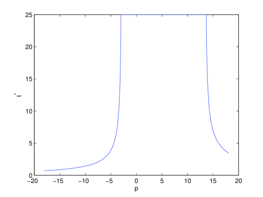
Figure 2: Moment explosion times ($\kappa_{1}=0.06$, $\kappa_{2}=0.04$, $\eta_{1}=0.2$, $\eta_{2}=0.1$, $\theta_{1}=1$, $\theta_{2}=0.3$, $\rho=-0.6$, $\gamma_{0}+\delta_{0}=0.02$, $\gamma_{1}+\delta_{1}=0.2$, $\gamma_{2}+\delta_{2}=0.2$).

A sample plot of the implied volatility surfaces for the two cases of positive probability of default and no default is given in Figure 3. For the calculation of implied volatilities we used the yield on a government bond as the interest rate in the Black–Scholes formula. As one would expect, credit risk contributes towards a higher implied volatility, especially at longer maturities or at extreme strikes. This effect can help explain why implied volatilities usually exceed realized volatilities.

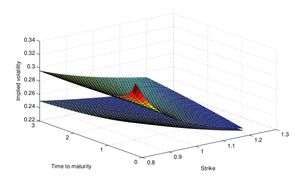
Figure 3: Implied volatility surfaces with positive probability of default (upper surface) vs. no default (lower surface). Parameters: $\kappa_{1}=0.06$, $\kappa_{2}=0.04$, $\eta_{1}=0.2$, $\eta_{2}=0.1$, $\theta_{1}=1$, $\theta_{2}=0.3$, $\rho=-0.6$, $c=0.02$ (no default: $c=0$), $\gamma_{1}=0.01$ (no default: $\gamma_{1}=0$), $\gamma_{2}=0.01$ (no default: $\gamma_{2}=0$), $d=0.01$, $\delta_{1}=0.1$, $\delta_{2}=0.1$, $X^{1}_{0}=0.05$, $X^{2}_{0}=0.03$, $X^{3}_{0}=0$.

5.2 Hedging

Denote by $\tilde{A}^{0}(t,z)$, $\tilde{B}^{0}_{1}(t,z)$ and $\tilde{B}^{0}_{2}(t,z)$ the solutions of the Riccati equations (5.4) for $c=\gamma_{1}=\gamma_{2}=0$ (no default). Then the price of a zero coupon government bond with maturity $t$ is given by

$$P^{0}_{t,x}=\exp(\tilde{A}^{0}(t,0)+\tilde{B}^{0}_{1}(t,0)x_{1}+\tilde{B}^{0}_{2}(t,0)x_{2}).$$

Assume there exists a $t>0$ such that

$$\partial_{x_{1}}c_{u,x}(k)\tilde{B}^{0}_{2}(u,0)-\partial_{x_{2}}c_{u,x}(k)\tilde{B}^{0}_{1}(u,0)\neq$$ (5.6)

$$[\tilde{B}^{0}_{1}(u,0)\tilde{B}_{2}(u,0)-\tilde{B}^{0}_{2}(u,0)\tilde{B}_{1}(u,0)][\partial_{x_{3}}c_{u,x}(k)-c_{u,x}(k)]$$

for all $0\leq u\leq t$ and $x\in D$. Then every European contingent claim can be hedged if the following four instruments can liquidly be traded: the stock, a zero coupon government bond, a zero coupon corporate bond and a call option with log strike $k$, the latter three all with maturity $t$.

Indeed, by Remarks 4.2 and 4.3, the hedging parameters are as follows:

• Stock: $H^{S,1}_{u,x}=H^{S,2}_{u,x}=0$, $H^{S,3}_{u,x}=e^{x_{3}}$, $D^{S}_{u,x}=-e^{x_{3}}$.

• Government bond: $H^{G,1}_{u,x}=\tilde{B}_{1}^{0}(u,0)P^{0}_{u,x}$, $H^{G,2}_{u,x}=\tilde{B}_{2}^{0}(u,0)P^{0}_{u,x}$, $H^{G,3}_{u,x}=0$, $D^{G}_{u,x}=0$.

• Corporate bond: $H^{B,1}_{u,x}=\tilde{B}_{1}(u,0)P_{u,x}$, $H^{B,2}_{u,x}=\tilde{B}_{2}(u,0)P_{u,x}$, $H^{B,3}_{u,x}=0$, $D^{B}_{u,x}=-P_{u,x}$.

• Call option: $H^{C,q}_{u,x}=\partial_{x_{q}}c_{u,x}(k)$, $q=1,2,3$, $D^{C}_{u,x}=-c_{u,x}(k)$,

and (5.6) is equivalent to

$$e^{x_{3}}P^{0}_{u,x}P_{u,x}\{-\partial_{x_{1}}c_{u,x}(k)\tilde{B}^{0}_{2}(u,0)+\partial_{x_{2}}c_{u,x}(k)\tilde{B}^{0}_{1}(u,0)$$

$$+[\tilde{B}^{0}_{1}(u,0)\tilde{B}_{2}(u,0)-\tilde{B}^{0}_{2}(u,0)\tilde{B}_{1}(u,0)][\partial_{x_{3}}c_{u,x}(k)-c_{u,x}(k)]\}\neq 0.$$

So the matrix

$$\left(\begin{array}[]{cccc}0&\tilde{B}^{0}_{1}(u,0)P^{0}_{u,x}&\tilde{B}_{1}(u,0)P_{u,x}&\partial_{x_{1}}c_{u,x}(k)\\ 0&\tilde{B}^{0}_{2}(u,0)P^{0}_{u,x}&\tilde{B}_{2}(u,0)P_{u,x}&\partial_{x_{2}}c_{u,x}(k)\\ e^{x_{3}}&0&0&\partial_{x_{3}}c_{u,x}(k)\\ -e^{x_{3}}&0&-P_{u,x}&-c_{u,x}(k)\end{array}\right).$$

has full rank, and the system (4.5) always has a solution.

Appendix A Proof of Theorem 4.1

It is shown in Theorem 8.1 of Filipovic and Mayerhofer [8] that there exists a measurable function $\sigma:D\to\mathbb{R}^{n\times n}$ satisfying (4.4) such that the SDE

$$dX_{t}=\tilde{b}(X_{t})dt+\sigma(X_{t})dW_{t}$$ (A.1)

has for each initial condition $x\in D$ a unique strong solution $X^{(0)}$. Now set $\tau_{0}:=0$ and define iteratively

$$\tau_{q} := \inf\left\{t>\tau_{q-1}:\int_{0}^{t}\int_{\mathbb{R}_{+}}k(X^{(q-1)}_{u-},z)N(du,dz)\neq 0\right\}$$ (A.2)

$$X^{(q)}_{t} := 1_{\left\{0\leq t<\tau_{q}\right\}}X^{(q-1)}_{t}+1_{\left\{\tau_{q}\leq t<\infty\right\}}Y^{(q)}_{t},$$

where $Y^{(q)}$ is the solution of the SDE (A.1) on $[\tau_{q},\infty)$ with initial condition

$$Y^{(q)}_{\tau_{q}}=X^{(q-1)}_{\tau_{q}}+k(X^{(q-1)}_{\tau_{q}-},z)N(\tau_{q},dz).$$

Since $X^{(q-1)}$ is RCLL and the intensity measure of $N$ is Lebesgue measure, it can be seen from (A.2) that $\tau_{q}>\tau_{q-1}$ a.s. So the process

$$X^{(\infty)}_{t}:=\sum_{q\geq 1}1_{\left\{\tau_{q-1}\leq t<\tau_{q}\right\}}X^{(q-1)}_{t}$$

is the unique strong solution of (4.3) on $[0,\tau_{\infty})$, where $\tau_{\infty}:=\lim_{q\to\infty}\tau_{q}$. It remains to show that $\tau_{\infty}=\infty$ and $X^{(\infty)}$ is a Feller process satisfying (H1)–(H2) with parameters $(a,\alpha,b,\beta,m,\mu)$. To do that we introduce the counting process

$$Z_{t}:=\sum_{q\geq 1}1_{\left\{t\geq\tau_{q}\right\}}.$$

By It$\hat{\textrm{o}}$’s formula,

$$f(X^{(\infty)}_{t\wedge\tau_{q}},Z_{t\wedge\tau_{q}})-\int_{0}^{t\wedge\tau_{q}}\tilde{\mathcal{A}}f(X^{(\infty)}_{u},Z_{u})du$$

is for all $f\in C^{2}_{c}(D\times\mathbb{R}_{+})$ and $q\geq 1$, a martingale, where

$$\tilde{\mathcal{A}}f(x,z) = \sum_{k,l=1}^{n}\left(a_{kl}+\left<\alpha_{\mathcal{I},kl},x_{\mathcal{I}}\right>\right)\frac{\partial^{2}f(x,z)}{\partial x_{k}\partial x_{l}}+\sum_{k=1}^{n}\left(b_{k}+\sum_{l=1}^{n}\beta_{kl}x_{l}\right)\frac{\partial f(x,z)}{\partial x_{k}}$$

$$+\int_{D\backslash\{0\}}\left(f(x+\xi,z+1)-f(x,z)-\left<\nabla_{\mathcal{J}}f(x,z),\chi_{\mathcal{J}}(\xi)\right>\right)\nu(d\xi)$$

$$+\sum_{i=1}^{m}\int_{D\backslash\{0\}}\left(f(x+\xi,z+1)-f(x,z)-\left<\nabla_{\mathcal{J}\cup\{i\}}f(x,z),\chi_{\mathcal{J}\cup\{i\}}(\xi)\right>\right)x_{i}\mu_{i}(d\xi).$$

But $\tilde{\cal A}$ is the infinitesimal generator of a regular affine process $\tilde{X}$ with values in $D\times\mathbb{R}_{+}$. So by Theorem 2.7 of Duffie et al. [6], $C^{2}_{c}(D\times\mathbb{R}_{+})$ is a core of $\tilde{\cal A}$, and it follows from Theorem 4.4.1 of Ethier and Kurtz [7] that the martingale problem for $\tilde{\mathcal{A}}\mid_{C^{2}_{c}(D\times\mathbb{R}_{+})}$ is well-posed. Moreover, the stopping times $\tau_{q}$ are exit times:

$$\tau_{q}=\inf\left\{t\geq 0:Z_{t}\notin[0,q-1/2)\right\}.$$

Therefore, one obtains from Theorem 4.6.1 of Ethier and Kurtz [7] that the stopped martingale problem corresponding to $\tilde{\cal A}\mid_{C^{2}_{c}(D\times\mathbb{R}_{+})}$ and $D\times[0,q-1/2)$ is well-posed for all $q$. Hence, $(X^{(\infty)}_{t\wedge\tau_{q}},Z_{t\wedge\tau_{q}})_{t\geq 0}$ has the same distribution as $(\tilde{X}_{t\wedge\tilde{\tau}_{q}})_{t\geq 0}$, where $\tilde{\tau}_{q}$ is the $q$-th jump time of $\tilde{X}$. Since $\tilde{X}$ is RCLL and $V_{M}+\sum_{i=1}^{m}V_{iM_{i}}X_{i,t}^{(\infty)}$ is the jump intensity of $Z$, we conclude that almost surely, the process $X^{(\infty)}_{t\wedge\tau_{\infty}}$ jumps at most finitely many times on compact time intervals. In particular, $\tau_{\infty}=\infty$, and Theorem 4.1 follows from Theorem 2.7 of Duffie et al. [6] since the first $n$ components of $\tilde{X}$ form a regular affine processes with infinitesimal generator ${\cal A}$ acting on $f\in C^{2}_{c}(D)$ like

$$\mathcal{A}f(x) = \sum_{k,l=1}^{n}\left(a_{kl}+\left<\alpha_{\mathcal{I},kl},x_{\mathcal{I}}\right>\right)\frac{\partial^{2}f(x)}{\partial x_{k}\partial x_{l}}+\left<b+\beta x,\nabla f(x)\right>$$

$$+\int_{D\backslash\{0\}}\left(f(x+\xi)-f(x)-\left<\nabla_{\mathcal{J}}f(x),\chi_{\mathcal{J}}(\xi)\right>\right)\nu(d\xi)$$

$$+\sum_{i=1}^{m}\int_{D\backslash\{0\}}\left(f(x+\xi)-f(x)-\left<\nabla_{\mathcal{J}\cup\{i\}}f(x),\chi_{\mathcal{J}\cup\{i\}}(\xi)\right>\right)x_{i}\mu_{i}(d\xi).$$

References

- [1] Andersen L., Piterbarg V. (2007). Moment explosions in stochastic volatility models. Finance and Stochastics, 11, 29–50.
- [2] Carr P., Madan D. (1999). Option valuation using the fast Fourier transform. Journal of Computational Finance 2(4), 61–73.
- [3] Carr P., Schoutens W. (2008). Hedging under the Heston model with jump-to-default. International Journal of Theoretical and Applied Finance 11(4), 403–414.
- [4] Cox J., Ingersoll J., Ross S. (1985). A theory of the term structure of interest rates. Econometrica 53, 385–467.
- [5] Dupire B. (1993). Model art. Risk 6(9), 118–124.
- [6] Duffie D., Filipovic D., Schachermayer W. (2003). Affine processes and applications in finance. Annals of Applied Probability 13(3), 984–1053.
- [7] Ethier S., Kurtz T. (2005). Markov Processes: Characterization and Convergence. John Wiley & Sons.
- [8] Filipovic D., Mayerhofer E. (2009). Affine diffusion processes: Theory and applications. Advanced Financial Modelling, volume 8 of Radon Series on Computational and Applied Mathematics, Walter de Gruyter, Berlin.
- [9] Heston S. (1993). A closed form solution for options with stochastic volatility with applications to bond and currency options. Review of Financial Studies 6(2), 327–343.
- [10] Ilyashenko Y., Yakovenko S. (2008). Lectures on Analytic Differential Equations. American Mathematical Society. Graduate Studies in Mathematics 86.
- [11] Keller-Ressel M. (2011). Moment explosions and long-term behavior of affine stochastic volatility models. Mathematical Finance, 21(1), 73–98.
- [12] Keller-Ressel M., Teichmann J., Schachermayer W. (2010). Affine processes are regular. Probability Theory and Related Fields, 1–21.
- [13] Lando D. (1998). On Cox processes and credit risky securities. Review of Derivatives Research 2, 99–120.
- [14] Lee R. (2004). The moment fomula for implied volatility at extreme strikes. Mathematical Finance 14(3), 469–480.
- [15] Lee R. (2005). Option pricing by transform methods: extensions, unification, and error control. Journal of Computational Finance 7(3), 51–86.
- [16] Lukacs E. (1970). Characteristic Functions. Charles Griffin & Co., Second Edition.
- [17] Neuberger A. (1994). The log contract. Journal of Portfolio Management 20(2), 74–80.
- [18] Spreij P., Veerman E. (2010). The affine transform formula for affine jump-diffusions with a general closed convex state space. Preprint.
- [19] Revuz D., Yor M. (1991). Continuous Martingales and Brownian Motion. Springer-Verlag, Berlin.
- [20] Sato K. (1999). Levy Processes and Infinitely Divisible Distributions. Cambridge University Press, Cambridge.
- [21] Stein E., Stein J. (1991). Stock price distributions with stochastic volatility: an analytic approach. Review of Financial Studies 4, 727–752.
- [22] Vasicek O. (1977). An equilibrium characterisation of the term structure. Journal of Financial Economics 5, 177 -188.