Nonlocal effective average action approach to crystalline phantom membranes

Abstract

We investigate the properties of crystalline phantom membranes, at the crumpling transition and in the flat phase, using a nonperturbative renormalization group approach. We avoid a derivative expansion of the effective average action and instead analyse the full momentum dependence of the elastic coupling functions. This leads to a more accurate determination of the critical exponents and further yields the full momentum dependence of the correlation functions of the in-plane and out-of-plane fluctuation. The flow equations are solved numerically for $D=2$ dimensional membranes embedded in a $d=3$ dimensional space. Within our approach we find a crumpling transition of second order which is characterized by an anomalous exponent $\eta_{c}\approx 0.63(8)$ and the thermal exponent $\nu\approx 0.69$. Near the crumpling transition the order parameter of the flat phase vanishes with a critical exponent $\beta\approx 0.22$. The flat phase anomalous dimension is $\eta_{f}\approx 0.85$ and the Poisson’s ratio inside the flat phase is found to be $\sigma_{f}\approx-1/3$. At the crumpling transition we find a much larger negative value of the Poisson’s ratio $\sigma_{c}\approx-0.71(5)$. We discuss further in detail the different regimes of the momentum dependent fluctuations, both in the flat phase and in the vicinity of the crumpling transition, and extract the crossover momentum scales which separate them.

I Introduction

Crystalline membranes have a fixed connectivity of their constituent particles and therefore a finite in-plane shear modulus which distinguishes them from fluid membranes membranebook . Physical crystalline membranes are two dimensional membranes embedded in three dimensional space and the embedding allows for out-of-plane fluctuations into the third dimension which are absent in a truly two-dimensional crystal. The coupling of the in-plane modes to the out-of-plane ones is responsible for a strong renormalization of the infrared (IR) character of both modes. Both acquire large anomalous dimensions which render the fluctuation of the local normals of the membrane finite and thus stabilize a flat phase in which the normals are ordered Nelson87 . The physics of such flat crystalline membranes has recently received renewed attention because of the discovery of graphene Castro09 , the thinnest possible crystalline membrane Meyer07 . At higher temperatures, the flat phase eventually becomes unstable and looses its orientational order of the normals at the crumpling transition Paczuski88 . Several approaches have been used to investigate the crumpling transition of phantom membranes. In contrast to real membranes, phantom membranes have no self-avoiding contact interaction which makes them more accessible to analytical approaches. Paczuski et al. studied a generalized model of a $D$-dimensional elastic manifold embedded in a $d$-dimensional space within a leading order $\epsilon=4-D$ expansion and found for $D=2$ ($\epsilon=2$) a first order transition for all $d<219$. The accuracy of this approach, which is well controlled only for small $\epsilon$, at $\epsilon=2$ is however in doubt. The results from the $\epsilon$ expansion disagree for $D=2$ with the results of a large $d$ expansion Paczuski89 ; Aronovitz89 and its extension, the selfconsistent screening approximation (SCSA) Doussal92 ; Gazit09 ; Zakharchenko10 where a continuous transition was found for $D=2$ and $d=3$. Further support for a continuous transition came from an elastic model with a constraint arising from infinitely large coupling constants for the stretching modes David88 , from a Monte Carlo (MC) renormalization group analysis Espriu96 , and from early MC simulations, see references in Bowick01rev . More recent MC simulations found however evidence for the coexistence of two separate phases at the critical temperature which would be consistent with a first order transition Kownacki02 ; Koibuchi04 , see also Koibuchi08 ; Nishiyama10 . A recent nonperturbative renormalization group (NPRG) analysis, based on a derivative expansion of the effective average action, could reproduce both the leading order results of the $\epsilon=4-D$ expansion as well as the leading order of a large $d$ expansion, within a unified framework Kownacki09 . The technique has recently also been applied to anisotropic membranes Essafi10 . For $D=2$ and $d=3$ evidence of a second order phase transition was found, but a weak first order transition could not be ruled out because of a weak dependence of the flow on the employed cutoff scheme.

Crystalline membranes are characterized by an anomalous elasticity in which none of the local elastic constants remain finite. The elasticity becomes fully nonlocal in the IR limit and the elastic coupling constants become coupling functions with a momentum dependence which for asymptotically small momenta is characterized by anomalous exponents. Here we present a NPRG analysis where the full momentum dependence of the coupling functions is kept, which allows for a more accurate analysis of the crumpling transition which we find to be continous. Our approach further allows to calculate the thermal fluctuations of the membrane beyond the asymptotic regime. We recover the results of Ref. Kownacki09 if the momentum dependence of the coupling functions is neglected. We previously applied our approach to compute the thermal fluctuations of free standing graphene Braghin10 and found excellent agreement for all momenta with MC simulations Fasolino07 ; Los09 . This analysis allowed to identify the characteristic scale of ripples in free standing graphene Meyer07 with the Ginzburg scale of the nonlinear elastic theory of crystalline membranes. The SCSA is also capable of accessing fluctuations at finite momenta and was applied to investigate the thermal fluctuations of graphene Zakharchenko10 , but proved to be, at finite momenta, less accurate than the NPRG approach. Here, we extend our approach and investigate in detail the behavior of a crystalline membrane inside the flat phase and at the crumpling transition critical point.

All approximations of our approach are included in our nonlocal ansatz of the effective average action and not at the level of the flow equations for irreducible vertices. Once the effective average action, which respects the full symmetry of the symmetric phase, is specified, the flow equations of the irreducible vertices are uniquely determined and can be solved exactly. In all previous schemes to calculate the full momentum dependence of self-energies of classical models (see Refs. phi4 for approaches for the $\Phi^{4}$ theory), some approximations were done in addition to the truncation of the effective average action which in principle can lead to a violation of Ward identities. Our approach is quite general and could also be applied to other physical models. Similar flow equations were derived for a model of interacting bosons Sinner10 . However, additional approximations had to be employed to solve the flow equations in which case the approach becomes equivalent to that presented in Sinner09 . The approach presented here assumes an ordered state but allows to approach and analyse the critical point from within the low temperature phase.

The structure of this manuscript is the following. In Sec. II we introduce and define the usual Landau-Ginzburg model of crystalline phantom membranes, which are membranes with no self-avoiding contact interaction. In Sec. III we present the derivation of our NPRG flow equations for the nonlocal elastic coupling functions. Expressions for the two longest diagrams of the flow equations can be found in the appendix. In Sec. IV we present results from a completely self-consistent numerical solution of the flow equations. We analyse the different scaling regimes in the momentum dependence of the out-of-plane and in-plane fluctuations and determine the critical exponents of the membrane both in the flat phase and at the crumpling transition fixed point. We further discuss the Poisson’s ratio, which is different at the crumpling transition and inside the flat phase. Finally, in Sec. V we present a summary and conclusion of this work.

II Landau-Ginzburg model

Our starting point is the usual Landau-Ginzburg model for crystalline phantom membranes (which have no contact interaction) Paczuski88 , with ${\cal H}={\cal H}^{\rm b}+{\cal H}^{\rm st}$. The bending part of the membranes is described by (silent indices are summed over)

$${\cal H}^{\rm b}=\frac{\tilde{\kappa}}{2}\int d^{D}{x}\left(\partial_{a}\partial_{a}{\bm{R}}\right)^{2}$$ (1a)

and the stretching is described by

$${\cal H}^{\rm st} = \int d^{D}x\big{[}\frac{{\tilde{r}}_{0}}{2}(\partial_{a}{\bm{R}})^{2}+\frac{\tilde{\mu}}{4}(\partial_{a}{\bm{R}}\cdot\partial_{b}{\bm{R}})^{2}$$ (1b)

$$+\frac{\tilde{\lambda}}{8}(\partial_{a}{\bm{R}}\cdot\partial_{a}{\bm{R}})^{2}\big{]}\,,$$

where ${\bm{R}}$ is a $D+1$ dimensional vector parameterizing the $D$ dimensional membrane which is embedded in a $d=D+1$ dimensional space. For notational convenience we restrict our analysis to $d=D+1$, it is however straightforward to extend our analysis to arbitrary $d$. In terms of the derivatives ${\bm{m}}_{a}=\partial_{a}{\bm{R}}$ the stretching part becomes

$${\cal H}^{\rm st} = \int d^{D}x\left[\frac{\tilde{r}_{0}}{2}\bm{m}_{a}\cdot\bm{m}_{a}+\frac{\tilde{\mu}}{4}(\bm{m}_{a}\cdot\bm{m}_{b})^{2}\right.$$ (2)

$$+\left.\frac{{\tilde{\lambda}}}{8}\left(\bm{m}_{a}\cdot\bm{m}_{a}\right)^{2}\right]\,,$$

and one can already anticipate a transition near $\tilde{r}_{0}\simeq 0$ from a flat configuration, which exists for negative $\tilde{r}_{0}$ and where the fields ${\bm{m}}_{a}$ acquire a finite expectation value ${\bm{m}}_{a,0}=\big{<}\bm{m}_{a}\big{>}\neq 0$, to a crumpled phase with $\big{<}\bm{m}_{a}\big{>}=0$. The stretching part Eq. (2) is appropriate for an isotropic membrane whose consituents particles have a fixed connectivity (such membranes are also refered to as tethered or polymerized membranes). A crystalline membrane has in general a lower symmetry and additional terms quartic in $\bm{m}_{a}$ are allowed, except for a two-dimensional hexagonal lattice Aronovitz89 . We here concentrate on models described by Eq. (2), appropriate for isotropic manifolds or membranes with hexagonal lattices and $D=2$.

For the flat phase, we introduce $J\neq 0$ as the magnitude of the order parameter which is defined as $\big{<}\bm{R}(\bm{x})\big{>}=Jx_{a}\bm{e}_{a}$ with $a=1\dots D$ and $\bm{e}_{a}$ are orthonormal vectors which span the plane of the membrane. Defining $U_{ab}=(\bm{m}_{a}\cdot\bm{m}_{b}-\bm{m}_{a,0}\cdot\bm{m}_{b,0})/2$ and $\bm{m}_{a,0}=J\bm{e}_{a}$, one can write Aronovitz89

$${\cal H}^{\rm st} =\int d^{D}x\Big{[}\tilde{\mu}\,U_{ab}^{2}+\frac{\tilde{\lambda}}{2}\,U_{aa}^{2}\Big{]}$$

$$\qquad+\int d^{D}x\Big{(}{\tilde{r}}_{0}+J^{2}[\tilde{\mu}+D\tilde{\lambda}/2]\Big{)}U_{aa}\,.$$ (3)

The last term has to vanish to guarantee thermodynamic stability and we thus have the mean field result

$$J_{\Lambda_{0}}^{2}=-\tilde{r}_{0}/[\tilde{\mu}_{\Lambda_{0}}+D\tilde{\lambda}_{\Lambda_{0}}/2]\,,$$ (4)

where the subscript $\Lambda_{0}$ indicates that this is a relation among the bare parameters which are assumed to be defined at some scale $\Lambda_{0}$.

III Derivation of the nonperturbative renormalization group flow equations

The NPRG approach is based on the exact flow equation of the effective average action $\Gamma_{\Lambda}$ Wetterich93

$$\frac{\partial\Gamma_{\Lambda}}{\partial\Lambda}=\frac{1}{2}{\rm Tr}\left[\left(\frac{\partial^{2}\Gamma_{\Lambda}}{\partial\phi\partial\phi^{\prime}}+R_{\Lambda}\right)^{-1}\frac{\partial R_{\Lambda}}{\partial\Lambda}\right]$$ (5)

where the fields $\phi,\phi^{\prime}$ here represent the components of the vector field ${\bm{R}}$ and the trace stands for a momentum integral and a sum over internal indices. The function $R_{\Lambda}$ is a regulator that removes IR divergences arising from modes with $k<\Lambda$ and will be specified below.

In principle, since the NPRG is not based on an expansion in a small parameter, the NPRG is not a-priori controlled. It has however been applied with much success to critical phenomena Berges02 and it usually reproduces leading order results of perturbative RG techniques such as $\epsilon$ expansions around the upper (or lower) critical dimension. For the case of crystalline membranes, the simplest possible NPRG ansatz Kownacki09 already reproduces the leading order results of both an $\epsilon=4-D$ expansion as well as a $1/d$ expansion. The approach presented here allows to calculate the momentum dependence of the membrane fluctuations which were found to be in perfect agreement with large scale MC simulations of unsuspended graphene Braghin10 . The NPRG technique thus seems to be quite reliable when applied to crystalline membranes.

III.1 Nonlocal elasticity

Our approximation of the effective average action consists of a nonlocal bending part $\Gamma^{\rm b}$, which is quadratic in the fields, and a nonlinear stretching part $\Gamma^{\rm st}$, which also includes quartic terms,

$$\Gamma_{\Lambda} = \Gamma_{\Lambda}^{\rm b}+\Gamma_{\Lambda}^{\rm st}$$ (6)

$$= \frac{1}{2}\int d^{D}x\ d^{D}x^{\prime}{\tilde{\kappa}}_{\Lambda}({\bm{x}}-{\bm{x}}^{\prime})\partial_{a}^{2}{\bm{R}}({\bm{x}})\partial_{b}^{2}{\bm{R}}({\bm{x}}^{\prime})$$

$$+\int d^{D}x\ d^{D}x^{\prime}\Big{[}{\tilde{\mu}}_{\Lambda}({\bm{x}}-{\bm{x}}^{\prime})U_{ab}({\bm{x}})U_{ab}({\bm{x}}^{\prime})$$

$$\qquad+\frac{1}{2}{\tilde{\lambda}}_{\Lambda}({\bm{x}}-{\bm{x}}^{\prime})U_{aa}({\bm{x}})U_{bb}({\bm{x}}^{\prime})\Big{]}.$$

This ansatz is simply a nonlocal generalization of the bare model defined via Eqs. (1a) and (3). Nonlocal correlations are known to be dominant in the IR limit of crystalline membranes where the Fourier-transformed coupling functions scale anomalously. Both in the flat phase and at the critical point of the crumpling transition, one has a pronounced hardening of the out-of plane fluctuations and a softening of the in-plane fluctuations. This is expressed by a divergent form of the bending coupling function and a vanishing of the bulk and shear modulus. In the flat phase one has $\tilde{\kappa}(q)\sim q^{-\eta_{f}}$ whereas the elastic coupling functions vanish as $\tilde{\mu}(q)\sim\tilde{\lambda}(q)\sim q^{\eta^{u}}$. Here, $\eta_{f}$ and $\eta^{u}$ are the anomalous exponents of the out-of plane fluctuations and the in-plane fluctuations, respectively. Note that these anomalous exponents are in fact not independent. Invariance of the original model under rotations implies a relation (Ward identity) among the anomalous dimensions Aronovitz89 ,

$$\eta^{u}=4-D-2\eta_{f}\,.$$ (7)

Since all fluctuations become anomalous in the IR limit, neither $\tilde{\kappa}(q)$, $\tilde{\mu}(k)$, nor $\tilde{\lambda}(k)$ are analytic functions in the limit $\Lambda\to 0$ and all fluctuations become nonlocal, a situation familiar from the behavior at a critical point of a continuous phase transition. In a leading order derivative expansion only the momentum independent parts of the coupling functions are kept, which is sufficient to extract their asymptotic momentum dependence by approximating $f_{\Lambda=0}(k)\approx f_{\Lambda=k}(0)$ where $f$ is any of the three coupling functions. We choose a more accurate approach, which also captures the corrections to the asymptotic behavior, and simply keep the full momentum dependence of the coupling functions for all $\Lambda$.

It is convenient to write the flow equation (5) of the functional $\Gamma_{\Lambda}$ as a flow equation of vertex functions, which can be obtained from a field expansion of both sides of (5). Since we are interested in the symmetry broken phase, we work with fields corresponding to the in-plane fluctuations ${\bm{u}}$ and out-of-plane fluctuations $h$ rather than the original $\bm{R}$ fields. These are introduced via the fluctuations of $\bm{m}_{a}$ around the ordered state, $\Delta{\bm{m}}_{a}=\partial_{a}\bm{R}-\bm{m}_{a,0}$ with $\Delta{\bm{m}}_{a}=(\partial_{a}{\bm{u}},\partial_{a}h)$ and ${\bm{m}}_{a,0}=J_{\Lambda}{\bm{e}}_{a}$. We therefore write the expansion

$$\Gamma_{\Lambda}[{\bm{u}},h]=\sum_{n,m=0}^{\infty}\frac{1}{n!m!}\iint\limits_{\begin{subarray}{c}{\bm{p}}_{1}\dots\bm{p}_{m}\\ {\bm{q}}_{1}\dots\bm{q}_{n}\end{subarray}}(2\pi)^{D}\delta\left(\sum_{i=1}^{n}{\bm{p}}_{i}+\sum_{i=1}^{m}{\bm{q}}_{i}\right)\\ \times\sum_{a_{1}\dots a_{m}=1}^{D}\Gamma^{(n+m)}_{\Lambda,{\underbrace{h\dots h}_{\mbox{\tiny n times}}}a_{1}\dots a_{m}}({\bm{q}}_{1},\dots,{\bm{q}}_{n};{\bm{p}}_{1},\dots,{\bm{p}}_{m})\\ \times h_{\bm{q}_{1}}\dots h_{\bm{q}_{n}}u_{\bm{p}_{1}}^{a_{1}}\dots u_{\bm{p}_{m}}^{a_{m}}\,,$$ (8)

where the momentum integrals are defined as

$$\int_{{\bm{q}}}=\int\frac{d^{D}q}{(2\pi)^{D}}\,.$$ (9)

The irreducible vertices entering Eq. (8) can be related to correlation functions. The simplest example is the Dyson equation which relates the one particle Green’s function to the irreducible self-energies. The Dyson equation for the Green’s function $G_{hh}$ of the $h$ field, with

$$\big{<}h_{\bm{q}}h_{-{\bm{q}}^{\prime}}\big{>}=V\delta_{{\bm{q}},{\bm{q}^{\prime}}}G_{hh}(q)\,,$$ (10)

where $V$ is the $D$-dimensional volume, is

$$G_{hh}^{-1}(q)=G_{0,\Lambda}^{-1}(q)+\Sigma_{hh}(q)\,.$$ (11)

The self-energy is of the form (here and below we suppress in our notation the explicit $\Lambda$ dependence of the coupling parameters $\tilde{\kappa}_{q}$ $\tilde{\mu}_{q}$, and $\tilde{\lambda}_{q}$)

$$\Sigma_{hh}(q)=\Gamma^{(2)}_{hh}({\bm{q}},-{\bm{q}})=({\tilde{\kappa}}_{q}-{\tilde{\kappa}}_{\Lambda_{0}})q^{4},$$ (12)

and the cutoff dependent non-interacting Green’s function is

$$G_{0,\Lambda}^{-1}(q)={\tilde{\kappa}}_{\Lambda_{0}}q^{4}+R_{\Lambda}(q),$$ (13)

where ${\tilde{\kappa}}_{\Lambda_{0}}$ denotes the bare and momentum independent value of the initial coupling constant ${\tilde{\kappa}}$ defined at the ultraviolet (UV) cutoff $\Lambda_{0}$. Here, we introduced the regulator function $R_{\Lambda}(q)$, which regulates the IR limit of the propagator in such a way that the IR divergence at $q\to 0$ is removed at finite $\Lambda$. Since we will later solve the NPRG flow equations numerically, we choose an analytic cutoff Kownacki09 ,

$$R_{\Lambda}(q)=\tilde{\kappa}_{\Lambda}^{(0)}\frac{q^{4}}{\exp[(q/\Lambda)^{4}]-1}\,,$$ (14)

where

$$\tilde{\kappa}_{\Lambda}^{(0)}=\tilde{\kappa}_{q=0}$$ (15)

is the $q=0$ component of the Fourier transform of $\tilde{\kappa}_{\Lambda}({\bm{x}})$. For finite $\Lambda$, we then have $\lim_{q\to 0}G_{0,\Lambda}^{-1}=\tilde{\kappa}_{\Lambda}^{(0)}\Lambda^{4}$ and $G_{0,\Lambda}$ is non-divergent for $q\to 0$.

The Green’s functions of the in-plane modes, defined via

$$\big{<}u^{a}_{\bm{k}}u^{b}_{-{\bm{k}}^{\prime}}\big{>}=V\delta_{{\bm{k}},{\bm{k}}^{\prime}}G_{ab}({\bm{k}}),$$ (16)

can be written in terms of transverse ($\perp$) and longitudinal ($\parallel$) components using the projectors

$$P^{\perp}_{ab}({\bm{k}}) =\delta_{ab}-k^{a}k^{b}/k^{2}\,,$$ (17a)

$$P^{\parallel}_{ab}({\bm{k}}) =k^{a}k^{b}/k^{2}\,.$$ (17b)

This yields

$$G_{ab}({\bm{k}})=G_{\perp}(k)P^{\perp}_{ab}({\bm{k}})+G_{\parallel}(k)P^{\parallel}_{ab}({\bm{k}})$$ (18)

with $G_{\alpha}^{-1}=G_{0,\Lambda}^{-1}+\Sigma_{\alpha}$ for $\alpha=\perp,\parallel$ and where the self-energies are defined as projections of

$$\Sigma_{ab}({\bm{k}})=\Gamma_{ab}^{(2)}({\bm{k}},-\bm{k})\,.$$ (19)

With the two-point irreducible vertex

$$\Gamma_{ab}^{(2)}(\bm{k}_{1},-\bm{k}_{2}) =J_{\Lambda}^{2}\Big{\{}\tilde{\mu}_{k_{1}}\big{(}\delta_{ab}{\bm{k}}_{1}\cdot{\bm{k}}_{2}+k_{2}^{a}k_{1}^{b}\big{)}+\tilde{\lambda}_{k_{1}}k_{1}^{a}k_{2}^{b}\Big{\}}$$

$$\quad+(\tilde{\kappa}_{k_{1}}-\tilde{\kappa}_{\Lambda_{0}})k_{1}^{2}k_{2}^{2}\,,$$ (20)

one finds the in-plane self-energies

$$\Sigma_{\perp}(k) = J_{\Lambda}^{2}{\tilde{\mu}}_{k}k^{2}+({\tilde{\kappa}}_{k}-{\tilde{\kappa}}_{\Lambda_{0}})k^{4},$$ (21a)

$$\Sigma_{\parallel}(k) = J_{\Lambda}^{2}(2{\tilde{\mu}}_{k}+{\tilde{\lambda}}_{k})k^{2}+({\tilde{\kappa}}_{k}-{\tilde{\kappa}}_{\Lambda_{0}})k^{4}.$$ (21b)

The effective average action Eq. (6) contains further three- and four-point vertices of the form (we use $k$ for momenta of $u$-fields and $p$ for momenta of $h$-fields)

$$\Gamma^{(3)}_{a_{1}a_{2}a_{3}}(\bm{k}_{1},\bm{k}_{2},\bm{k}_{3}) =\frac{-iJ_{\Lambda}}{2}\sum_{(\alpha\beta\gamma)={\cal P}_{123}}\big{\{}2\tilde{\mu}_{k_{\alpha}}(\bm{k}_{\alpha}\cdot\bm{k}_{\beta})k_{\gamma}^{a_{\alpha}}$$

$$\quad+\tilde{\lambda}_{k_{\alpha}}(\bm{k}_{\beta}\cdot\bm{k}_{\gamma})k_{\alpha}^{a_{\alpha}}\big{\}}\delta_{a_{\beta},a_{\gamma}}$$ (22a)

$$\Gamma^{(3)}_{hha}(\bm{p}_{1},\bm{p}_{2};\bm{k}) =-iJ_{\Lambda}\big{\{}\tilde{\mu}_{k}\big{[}(\bm{p}_{1}\cdot\bm{k})p_{2}^{a}+(\bm{p}_{2}\cdot\bm{k})p_{1}^{a}\big{]}$$

$$\quad+\tilde{\lambda}_{k}(\bm{p}_{1}\cdot\bm{p}_{2})k^{a}\big{\}}\,,$$ (22b)

$$\Gamma^{(4)}_{a_{1}\dots a_{4}}(\bm{k}_{1}\dots\bm{k}_{4})=\frac{1}{8}\sum\limits_{\begin{subarray}{c}(\alpha\beta\gamma\delta)\\ ={\cal P}_{1234}\end{subarray}}\big{\{}2\tilde{\mu}_{k_{\alpha\beta}}(\bm{k}_{\alpha}\cdot\bm{k}_{\gamma})(\bm{k}_{\beta}\cdot\bm{k}_{\delta})\\ \,\,\,\qquad+\tilde{\lambda}_{k_{\alpha\beta}}(\bm{k}_{\alpha}\cdot\bm{k}_{\beta})(\bm{k}_{\gamma}\cdot\bm{k}_{\delta})\big{\}}\delta_{a_{\alpha},a_{\beta}}\delta_{a_{\gamma},a_{\delta}}\,,$$ (22c)

$$\Gamma^{(4)}_{hha_{1}a_{2}}(\bm{p}_{1},\bm{p}_{2};\bm{k}_{1},\bm{k}_{2})=\big{\{}\tilde{\mu}_{p_{12}}\big{[}(\bm{p}_{1}\cdot\bm{k}_{1})(\bm{p}_{2}\cdot\bm{k}_{2})\\ +(\bm{p}_{1}\cdot\bm{k}_{2})(\bm{p}_{2}\cdot\bm{k}_{1})\big{]}+\tilde{\lambda}_{p_{12}}(\bm{p}_{1}\cdot\bm{p}_{2})(\bm{k}_{1}\cdot\bm{k}_{2})\big{\}}\delta_{a_{1},a_{2}}\,,$$ (22d)

$$\Gamma^{(4)}_{hhhh}(\bm{p}_{1}\dots\bm{p}_{4})\\ =\frac{1}{8}\sum\limits_{\begin{subarray}{c}(\alpha\beta\gamma\delta)={\cal P}_{1234}\end{subarray}}\big{\{}2\tilde{\mu}_{p_{\alpha\beta}}+\tilde{\lambda}_{p_{\alpha\gamma}}\big{\}}(\bm{p}_{\alpha}\cdot\bm{p}_{\gamma})(\bm{p}_{\beta}\cdot\bm{p}_{\delta})\,,$$ (22e)

where $k_{\alpha\beta}=|{\bm{k}}_{\alpha}+{\bm{k}}_{\beta}|$ and $\sum_{(\alpha\beta\gamma)={\cal P}_{123}}$ denotes a summation over all permutations of $(123)$. The subscript $h$ refers to $h$-fields while subscripts $a$ and $a_{i}$ refer to ${u}$-fields. Since we neglect all irreducible correlations not explicitely included in Eq. (6), higher order vertices, with more than four legs, do not appear in our approximation. Finally, we shall also need the single scale propagators which are defined via

$${\dot{G}}_{ab} =-\Big{(}G_{\perp}^{2}P_{ab}^{\perp}+G_{\parallel}^{2}P_{ab}^{\parallel}\Big{)}\partial_{\Lambda}R_{\Lambda}\,,$$ (23a)

$${\dot{G}}_{hh} =-G_{hh}^{2}\partial_{\Lambda}R_{\Lambda}\,.$$ (23b)

III.2 Flow equations for momentum dependent vertices

We will now derive the flow equations for the order parameter $J_{\Lambda}$ and the coupling functions $\tilde{\kappa}_{q}$, $\tilde{\mu}_{q}$ and $\tilde{\lambda}_{q}$. The flow of $J_{\Lambda}^{2}$ can be extracted from the flow equation of the one-point vertex of the ${u}$-fields whereas the other three coupling functions can be extracted from the flow equations of the self-energies. All higher order vertices presented in Sec. III.1 are completely determined by $J_{\Lambda}^{2}$, $\tilde{\kappa}_{q}$, $\tilde{\mu}_{q}$ and $\tilde{\lambda}_{q}$, and the flow equations for the one- and two-point vertices are thus closed.

The only approximation of our approach is the approximation for the effective average action as expressed through Eq. (6) and in the derivation below no further approximation is required. The resulting flow equations are uniquely determined by Eqs. (5) and (6) and obey the full symmetry of Eq. (6).

The NPRG flow of the one-point function $\Gamma_{a}^{(1)}$ is

$$\partial_{\Lambda}\Gamma_{a}^{(1)}({\bm{k}}) =-i(\partial_{\Lambda}J_{\Lambda})(2\pi)^{D}\delta^{(D)}({\bm{k}})\frac{\partial}{\partial{k^{\prime}}^{b}}\Gamma^{(2)}_{ab}({\bm{k}},-\bm{k}^{\prime})\Big{|}_{\bm{k}^{\prime}=\bm{k}}$$

$$+\frac{1}{2}\int_{{\bm{q}}}\big{\{}\dot{G}_{hh}(q)\Gamma^{(3)}_{hha}({\bm{q}},-{\bm{q}};{\bm{k}})$$

$$\qquad+\dot{G}_{bc}({\bm{q}})\Gamma^{(3)}_{abc}({\bm{k}},{\bm{q}},-{\bm{q}})\big{\}}(2\pi)^{D}\delta^{(D)}({\bm{k}})\,,$$ (24)

where we used the $\bm{k}$-space representation of the order parameter field

$$\big{<}R^{a}\big{>}(\bm{k})=-iJ_{\Lambda}(2\pi)^{D}\delta^{(D)}(\bm{k})\frac{\partial}{\partial{k^{a}}}\,.$$ (25)

Figure 1: (Color online) Diagrammatic representation of the flow equation which determines the flow of the order parameter and which arises from the vanishing flow of the one-point vertex Schuetz06 . Wavy lines correspond to $G_{ab}$ propagators and solid lines to $G_{hh}$. Lines with a dash correspond to single-scale propagators. The small open circle with a dot denotes a derivative of the order parameter with respect to $\Lambda$.

The condition $\partial_{\Lambda}\Gamma_{a}^{(1)}(\bm{k})=0$ then yields an equation which is shown diagrammatically in Fig. 1 and from which the flow of the order parameter can be determined. One finds

$$\partial_{\Lambda}J_{\Lambda}^{2}=\frac{K_{D}}{[2\tilde{\mu}_{0}+D{\tilde{\lambda}}_{0}]D}\int dq\;q^{D+1}\Big{\{}(D-1)\dot{G}_{\perp}(q)\\ \times[2\tilde{\mu}_{q}+2\tilde{\mu}_{0}+D{\tilde{\lambda}}_{0}]\\ +\dot{G}_{\parallel}(q)\left[2(2\tilde{\mu}_{q}+\tilde{\mu}_{0})+2{\tilde{\lambda}}_{q}+D{\tilde{\lambda}}_{0}\right]\\ +\dot{G}_{hh}(q)[2\tilde{\mu}_{0}+D{\tilde{\lambda}}_{0}]\Big{\}}\,,$$ (26)

where

$$K_{D}=\frac{1}{2^{D-1}\pi^{D/2}\Gamma[D/2]}\,.$$ (27)

The flow of $\tilde{\kappa}(q)$ follows directly from the flow equation for $\Sigma_{hh}$. The flow equation is shown diagrammatically in Fig. 2 and is given by the expression

$$\partial_{\Lambda}\Sigma_{hh}(k) =k^{4}\partial_{\Lambda}{\tilde{\kappa}}_{k}$$

$$=k^{2}\frac{\partial_{\Lambda}J_{\Lambda}^{2}}{2}(2\tilde{\mu}_{0}+D{\tilde{\lambda}}_{0})$$

$$\quad+[S_{hh}^{h}(k)+S_{hh}^{u}(k)]/2-S_{hh}^{uh}(k)-S_{hh}^{hu}(k)\,.$$ (28)

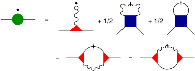
Figure 2: (Color online) Diagrams which enter the flow of the self-energy $\Sigma_{hh}$ of the out-of-plane fluctuations. The solid dot above the self-energy on the l.h.s. denotes a derivative w.r.t. $\Lambda$, the other symbols are defined in the caption of Fig. 1.

The diagrams entering the flow of $\Sigma_{hh}(k)$ are

$$S^{h}_{hh}(k) =\int_{{\bm{q}}}\dot{G}_{hh}(q)\Gamma_{hhhh}^{(4)}({\bm{k}},-{\bm{k}},{\bm{q}},-{\bm{q}})\,,$$ (29a)

$$S^{u}_{hh}(k) =\int_{{\bm{q}}}\dot{G}_{ab}({\bm{q}})\Gamma_{hhab}^{(4)}({\bm{k}},-{\bm{k}};{\bm{q}},-{\bm{q}})\,,$$ (29b)

$$S^{hu}_{hh}(k) =\int_{{\bm{q}}}\dot{G}_{hh}({\bm{q}})G_{ab}({\bm{q}}^{\prime})$$

$$\qquad\times\Gamma_{hha}^{(3)}({\bm{k}},{\bm{q}};-{\bm{q}}^{\prime})\Gamma_{hhb}^{(3)}(-{\bm{k}},-{\bm{q}};{\bm{q}}^{\prime})\,,$$ (29c)

$$S^{uh}_{hh}(k) =\int_{{\bm{q}}}\dot{G}_{ab}({\bm{q}})G_{hh}({\bm{q}}^{\prime})$$

$$\qquad\times\Gamma_{hha}^{(3)}({\bm{k}},-{\bm{q}}^{\prime};{\bm{q}})\Gamma_{hhb}^{(3)}(-{\bm{k}},{\bm{q}}^{\prime};-{\bm{q}})\,,$$ (29d)

where the direction of ${\bm{k}}$ on the right hand side of these equations can be chosen arbitrarily since the diagrams only depend on the modulus $k$, and ${\bm{q}}^{\prime}={\bm{k}}+{\bm{q}}$. The subscript $hh$ indicates two external $h$-legs and the superscript indicates the composition of the internal loop, i.e. $S_{hh}^{h}$ indicates a diagram where the loop consists of one $h$-line. $S_{hh}^{uh}$ differs from $S_{hh}^{hu}$ in that in $S_{hh}^{uh}$ the single-scale propagator is a $u$-line whereas in $S_{hh}^{hu}$ it is a $h$-line. With the vertices given in Eqs. (22-22e) these diagrams become

$$S^{h}_{hh}(k) =k^{2}\int_{\bm{q}}q^{2}\dot{G}_{hh}(q)$$

$$\quad\times\big{[}2\tilde{\mu}_{q^{\prime}}+{\tilde{\lambda}}_{0}+2y^{2}(\tilde{\mu}_{0}+\tilde{\mu}_{q^{\prime}}+{\tilde{\lambda}}_{q^{\prime}})\big{]}\,,$$ (30a)

$$S^{u}_{hh}(k) =k^{2}\int_{\bm{q}}q^{2}[\dot{G}_{\perp}(q)(D-1)+\dot{G}_{\parallel}(q)](2y^{2}\tilde{\mu}_{0}+{\tilde{\lambda}}_{0})\,,$$ (30b)

$$S_{hh}^{hu}(k) =k^{2}J_{\Lambda}^{2}\int_{{\bm{q}}}q^{2}\dot{G}_{hh}(q^{\prime})\Big{\{}G_{\perp}(q)\tilde{\mu}_{q}^{2}(1-y^{2})(2ky+q)^{2}$$

$$\qquad+G_{\parallel}(q)\big{[}2\tilde{\mu}_{q}y(q+ky)+\tilde{\lambda}_{q}(k+qy)\big{]}^{2}\Big{\}}\,,$$ (30c)

$$S_{hh}^{uh}(k) =k^{2}J_{\Lambda}^{2}\int_{{\bm{q}}}q^{2}G_{hh}(q^{\prime})\Big{\{}\dot{G}_{\perp}(q)\tilde{\mu}_{q}^{2}(1-y^{2})(2ky+q)^{2}$$

$$\qquad+\dot{G}_{\parallel}(q)\big{[}2\tilde{\mu}_{q}y(q+ky)+\tilde{\lambda}_{q}(k+qy)\big{]}^{2}\Big{\}}\,.$$ (30d)

Note that each of the diagrams given in Eqs. (30-30d) is to leading order quadratic in $k$. However, their sum cancels to leading order exactly the first term in Eq. (III.2) so that the overall leading term of the flow of $\Sigma_{hh}$ is indeed quartic in $k$.

Figure 3: (Color online) Diagrams which determine the flow of the self-energy $\Sigma_{ab}$ of the in-plane fluctuations. The symbols are defined as in Figs. 1 and 2.

Finally, using the flow equation of $\Sigma_{ab}({\bm{k}})$, one can determine the flow of $\tilde{\mu}_{k}$ and $\tilde{\lambda}_{k}$. The flow of $\Sigma_{ab}({\bm{k}})$ has the form (see Fig. 3)

$$\partial_{\Lambda}{\Sigma}_{ab}({\bm{k}}) =\big{[}(D\tilde{\lambda}_{0}+2\tilde{\mu}_{k}+2\tilde{\mu}_{0})k^{2}\delta_{ab}$$

$$\qquad+2(\tilde{\lambda}_{k}+\tilde{\mu}_{k})k^{a}k^{b}\big{]}\partial_{\Lambda}J_{\Lambda}+(1/2)S_{ab}^{u}({\bm{k}})$$

$$\qquad+(1/2)S_{ab}^{h}({\bm{k}})-S_{ab}^{hh}({\bm{k}})-S_{ab}^{uu}({\bm{k}})\,,$$ (31)

where the first term arises from the diagram with one external leg coupled to the derivative of the order parameter field and $S_{ab}^{u}({\bm{k}})$ stands for a diagram with external $u$-lines with flavors $a,b$ and momentum $k$, and an internal loop which consists of one $u$-line. Similarly, for $S_{ab}^{uu}({\bm{k}})$ the internal loop consists of two $u$-lines and for $S_{ab}^{hh}({\bm{k}})$ the internal loop consists of two $h$-lines. The analytic expressions for these diagrams are

$$S_{ab}^{h}({\bm{k}}) =\int_{{\bm{q}}}\dot{G}_{hh}(q)\Gamma^{(4)}_{hhab}({\bm{k}},-{\bm{k}};{\bm{q}},-{\bm{q}})\,,$$ (32a)

$$S_{ab}^{u}({\bm{k}}) =\int_{{\bm{q}}}\dot{G}_{cd}({\bm{q}})\Gamma_{abcd}^{(4)}({\bm{k}},-{\bm{k}},{\bm{q}},-{\bm{q}})\,,$$ (32b)

$$S_{ab}^{hh}({\bm{k}}) =\int_{{\bm{q}}}\dot{G}_{hh}(q)G_{hh}(q^{\prime})$$

$$\qquad\times\Gamma_{hha}^{(3)}({\bm{q}},-{\bm{q}}^{\prime};{\bm{k}})\Gamma_{hhb}^{(3)}(-{\bm{q}},{\bm{q}}^{\prime};-{\bm{k}})\,,$$ (32c)

$$S_{ab}^{uu}({\bm{k}}) =\int_{{\bm{q}}}\dot{G}_{cd}({\bm{q}}){G}_{ef}({\bm{q}}^{\prime})$$

$$\qquad\times\Gamma_{ace}^{(3)}({\bm{k}},{\bm{q}},-{\bm{q}}^{\prime})\Gamma_{bdf}^{(3)}(-{\bm{k}},-{\bm{q}},{\bm{q}}^{\prime})\,,$$ (32d)

where ${\bm{q}}^{\prime}={\bm{k}}+{\bm{q}}$. After projecting on transversal and longitudinal components, one finds from Eq. (III.2) and the form of the projected self-energies in Eqs. (21a) and (21b)

$$k^{2}\partial_{\Lambda}\tilde{\mu}_{k} =k^{2}(\tilde{\mu}_{0}+D\tilde{\lambda}_{0}/2)\partial_{\Lambda}J_{\Lambda}^{2}+(1/2)S_{\perp}^{u}(k)$$

$$\quad+(1/2)S_{\perp}^{h}(k)-S_{\perp}^{hh}(k)-S_{\perp}^{uu}(k)$$

$$\quad-k^{4}\partial_{\Lambda}\tilde{\kappa}_{k}\,,$$ (33a)

$$k^{2}\partial_{\Lambda}(2\tilde{\mu}_{k}+\tilde{\lambda}_{k}) =k^{2}(\tilde{\mu}_{0}+D\tilde{\lambda}_{0}/2)\partial_{\Lambda}J_{\Lambda}^{2}+(1/2)S_{\parallel}^{u}(k)$$

$$\quad+(1/2)S_{\parallel}^{h}(k)-S_{\parallel}^{hh}(k)-S_{\parallel}^{uu}(k)$$

$$\quad-k^{4}\partial_{\Lambda}\tilde{\kappa}_{k}\,.$$ (33b)

The projected diagram $S_{\alpha}^{u}(k)$, with $\alpha=\perp$ or $\parallel$, is defined via $P_{ac}^{\alpha}({\bm{k}})S_{cb}^{u}({\bm{k}})=P_{ab}^{\alpha}({\bm{k}})S_{\alpha}^{u}(k)$ and the other projected diagrams are similarly defined. With $y={\bm{k}}\cdot{\bm{q}}/kq$, the transverse projected diagrams have the form

$$S_{\perp}^{h}(k) =k^{2}\int_{{\bm{q}}}q^{2}\dot{G}_{hh}(q)\big{[}2\tilde{\mu}_{0}y^{2}+{\tilde{\lambda}}_{0}\big{]}\,,$$ (34a)

$$S_{\perp}^{u}(k) =\frac{k^{2}}{D-1}\int_{{\bm{q}}}q^{2}\Big{\{}\big{[}\dot{G}_{\perp}(q)(D-1)+\dot{G}_{\parallel}(q)\big{]}$$

$$\qquad\times(D-1)\big{[}2\tilde{\mu}_{0}y^{2}+{\tilde{\lambda}}_{0}\big{]}$$

$$\quad+\big{[}\dot{G}_{\perp}(q)(D-2+y^{2})+\dot{G}_{\parallel}(q)(1-y^{2})\big{]}$$

$$\qquad\times 2\big{[}\tilde{\mu}_{q^{\prime}}(1+y^{2})+{\tilde{\lambda}}_{q^{\prime}}y^{2}\big{]}\Big{\}}\,,$$ (34b)

$$S_{\perp}^{hh}(k) =\frac{J_{\Lambda}^{2}k^{2}}{D-1}\int_{{\bm{q}}}q^{2}\dot{G}_{hh}(q)G_{hh}(q^{\prime})$$

$$\qquad\times\tilde{\mu}_{k}^{2}(k+2yq)^{2}(1-y^{2})\,.$$ (34c)

The expression of the diagram $S_{\perp}^{uu}(k)$ is rather long and can be found in the appendix. The longitudinal projections are

$$S_{\parallel}^{h}(k) =S_{\perp}^{h}(k)\,,$$ (35a)

$$S_{\parallel}^{u}(k) =k^{2}\int_{{\bm{q}}}q^{2}\Big{\{}\big{[}\dot{G}_{\perp}(q)(D-1)+\dot{G}_{\parallel}(q)\big{]}$$

$$\qquad\times(D-1)\big{[}2\tilde{\mu}_{0}y^{2}+{\tilde{\lambda}}_{0}\big{]}$$

$$\quad+\big{[}\dot{G}_{\perp}(q)(1-y^{2})+\dot{G}_{\parallel}(q)y^{2}\big{]}$$

$$\qquad\times 2\big{[}\tilde{\mu}_{q^{\prime}}(1+y^{2})+{\tilde{\lambda}}_{q^{\prime}}y^{2}\big{]}\Big{\}}\,,$$ (35b)

$$S_{\parallel}^{hh}(k) =J_{\Lambda}^{2}k^{2}\int_{{\bm{q}}}q^{2}\dot{G}_{hh}(q)G_{hh}(q^{\prime})$$

$$\qquad\times\big{[}\tilde{\lambda}_{k}(q+ky)+2\tilde{\mu}_{k}(k+qy)y\big{]}^{2}\,,$$ (35c)

and the expression for $S_{\parallel}^{uu}(k)$ is given in the appendix.

IV Results

The set of Eqs. (26), (III.2), (33), and (33b) form a set of coupled integrodifferential equations which we solve numerically. We are mainly interested in the behavior of the $D=2$ dimensional membrane embedded in three dimensional space near its critical regime. For simplicity we use as initial conditions momentum independent coupling constants,

$$\tilde{\kappa}_{\Lambda_{0}}=1\,\,\,\mbox{and}\,\,\,\tilde{\mu}_{\Lambda_{0}}=\tilde{\lambda}_{\Lambda_{0}}=\Lambda_{0}^{2}\,.$$ (36)

The initial mean field value of the order parameter $J_{\Lambda_{0}}$ will be tuned to reach the critical point of the crumpling transition. Since our approach breaks down within the crumpled phase, we can approach the critical point only from the flat phase. We begin by discussing the properties of the flat phase.

IV.1 Flat phase

The flat phase is characterized by a finite order parameter $J=\lim_{\Lambda\to 0}J_{\Lambda}$. Asymptotically, the out-of-plane fluctuations are governed by the anomalous dimension $\eta_{f}$ associated with the flat phase fixed point,

$$G_{hh}(k)\sim q^{-(4-\eta_{f})}\,,$$ (37)

while the in-plane fluctuations are governed by the anomalous dimension $\eta^{u}$,

$$G_{\perp}(q)\sim G_{\parallel}(q)\sim q^{-(2+\eta^{u})}\,.$$ (38)

We can extract the flow of the anomalous dimension from the leading $q=0$ term of $\tilde{\kappa}(q)$,

$$\Lambda\partial_{\Lambda}\tilde{\kappa}^{(0)}_{\Lambda}=-\eta_{\Lambda}\tilde{\kappa}^{(0)}_{\Lambda}\,,$$ (39)

where $\tilde{\kappa}_{\Lambda}^{(0)}=\tilde{\kappa}_{q=0}$. In accordance with the derivative expansion result Kownacki09 and recent MC simulations of graphene Los09 we find for $D=2$ the anomalous dimension $\eta_{f}\approx 0.85$ which yields $\eta^{u}\approx 0.30$. These values are also close to the SCSA result $\eta_{f}\approx 0.821$ Doussal92 and the MC results $\eta\approx 0.750(5)$ Bowick96 and $\eta\approx 0.81(3)$ Zhang93 . A typical flow of the anomalous dimension far away from the critical point is shown in the upmost curve in Fig. 4. There is some scatter of the numerical data for $\eta_{\Lambda}$ since $\eta_{\Lambda}$ has to be extracted from the $\Lambda$ derivative of the very small $q$ dependence of $\tilde{\kappa}_{q}$. The numerical noise in the function $\tilde{\kappa}_{q}$ itself is however very small. The anomalous scaling of the propagators, as expressed through Eqs. (37) and (38), is observable only for momenta smaller than the Ginzburg scale $q_{G}$. This scale can be obtained perturbatively and has for $D=2$ the form membranebook ; Nelson87

$$q_{G}\approx[3\tilde{K}_{0}/(2\pi)]^{1/2}/(4{\tilde{\kappa}})$$ (40)

where

$$\tilde{K}_{0}=4J_{\Lambda_{0}}^{2}{\tilde{\mu}}({\tilde{\mu}}+{\tilde{\lambda}})/(2{\tilde{\mu}}+{\tilde{\lambda}})\,$$ (41)

is the (bare) Young’s modulus. Since for all our calculations we used Eq. (36) and similar values of $J_{\Lambda_{0}}^{2}\approx 0.5$, one finds for all the data we present here to a good approximation a common Ginzburg scale of the order of $q_{G}\approx 0.2\Lambda_{0}$. For $q\ll q_{G}$ the Green’s functions are strongly renormalized and the flat phase fixed point scaling regime appears. This behavior is clearly seen in both $G_{hh}(q)$ and $G_{\perp}(q)$, see the lowest curves in Figs. 5 and 6, which where obtained for $J_{\Lambda_{0}}^{2}=1/2$ or $\delta J=J_{\Lambda_{0}}-J_{c}\approx 0.08$, where $J_{c}$ is the critical $J_{\Lambda_{0}}$ value of the crumpling transition for the initial values of the elastic constants stated in Eq. (36). In the small $q$ limit, we find $G_{hh}(q)\propto 1/q^{4-\eta_{f}}$, as expected from the analysis of the flow of $\eta_{\Lambda}$. Similarly, for the in-plane correlation functions we find $G_{\alpha}\propto 1/q^{2+\eta^{u}}$ with $\alpha=\perp,\parallel$ and an anomalous exponent $\eta^{u}=2-2\eta_{f}$, as expected from the Ward identity Eq. (7).

The upper curve in Fig. 7 shows the flow of the Poisson’s ratio

$$\sigma_{\Lambda}=\frac{\tilde{\lambda}_{q=0}}{2\tilde{\mu}_{q=0}+\tilde{\lambda}_{q=0}}\,,$$ (42)

which in the flat phase is known to acquire a negative value for $\Lambda\to 0$. For $\Lambda\to 0$ one finds in the flat phase a Poisson’s ratio $\sigma_{f}\approx-1/3$, as in the NPRG derivative expansion Kownacki09 , and in perfect agreement with both the SCSA result Doussal92 and MC results for phantom membranes Falcioni97 and in good agreement with MC results for self-avoiding membranes Bowick01 .

Figure 4: Flow of the critical exponent $\eta$ for different initial values of $J_{\Lambda_{0}}^{2}$ (solid dots). For finite $J^{2}=\lim_{\Lambda\to 0}J_{\Lambda}^{2}$, $\eta_{\Lambda}$ saturates at the flat phase fixed point value $\eta_{f}\approx 0.85$, this value is indicated by the upper vertical line. At the crumpling transition (with $J_{\Lambda_{0}}=J_{c}$) $\eta_{\Lambda}$ saturates at the critical fixed point value $\eta_{c}\approx 0.638$ (see curve 1), this value is indicated by the lower vertical line. The values for $(J_{\Lambda_{0}}^{2}-J_{c}^{2})/J_{c}^{2}$ are $8.0\times 10^{-7}$ (curve 2), $3.0\times 10^{-5}$ (curve 3), $5.0\times 10^{-4}$ (curve 4), $9.1\times 10^{-3}$ (curve 5), and $1.9\times 10^{-1}$ (curve 6).

IV.2 Behavior close to and at the crumpling transition

Upon lowering the initial value of $J_{\Lambda_{0}}^{2}$, we can tune the membrane towards the critical regime of the crumpling transition. Exactly at the crumpling transition the value of the anomalous dimension is changed from the flat phase fixed point value. The lowest curve in Fig. 4 shows the flow of $\eta_{\Lambda}$ at the critical value of $J_{\Lambda_{0}}^{2}$. One can clearly observe a fixed point value $\eta_{c}$ which is different from the one obtained for the flat phase. We find a value

$$\eta_{c}\approx 0.63(8)\,,$$ (43)

which is larger than the SCSA result $\eta_{c}=0.535$ Doussal92 , and the value $\eta_{c}=0.47$ from a MC renormalization group analysis Espriu96 , but rather close to the large $D$ result $\eta=2/3$ and the derivative expansion approach to the NPRG Kownacki09 $\eta\approx 0.627$, obtained with a sharp cutoff. In the derivative expansion, a weak dependence of the critical properties on the form of the regulator was reported. In our numerical approach, we are for reasons of numerical stability restricted to analytical regulators note1 . We would expect however a much weaker dependence on the form of the regulator in our approach since we keep the entire momentum dependence of all two-point vertices and since the regulator, for a given $\Lambda$, only affects the momentum dependence of the two-point functions.

Figure 5: The correlation function $G_{hh}(k)$ (solid lines) for different values of $J_{\Lambda_{0}}^{2}-J_{c}^{2}$ (curves are multiplied with $k^{3}$ for easier visibility of the different scaling regimes). At the critical point of the crumbling transition (upmost curve) a single crossover from the perturbative scaling to a critical scaling with $\eta_{c}\approx 0.63(8)$ is observed. Slightly away from criticality (middle curve), $G_{hh}$ enters at small momenta the flat phase fixed point scaling with $\eta_{f}\approx 0.85$. Even further away (lower curve), the intermediate regime, where $G_{hh}$ obeys critical scaling, disappears and a direct crossover from perturbative to flat phase fixed point scaling is observed. Dashed lines indicate the different scaling behaviors.

A small distance $J_{\Lambda_{0}}^{2}-J_{c}^{2}>0$ away from the critical value $J_{c}^{2}$, $\eta_{\Lambda}$ initially approaches the critical fixed point value $\eta_{c}$ but deviates from it in the IR limit to finally saturate at the flat phase fixed point. This behavior can be seen for different values of $J_{\Lambda_{0}}^{2}>J_{c}^{2}$ in Fig. 4.

The behavior of the Green’s function $G_{hh}(q)$ at the critical point is shown in Fig. 5. There is again a crossover from perturbative scaling to anomalous scaling near $q_{G}$, similar as in the flat phase. The anomalous scaling is now the critical scaling with $\eta=\eta_{c}$. As expected from an analysis of the flow of the critical exponent, there is a second crossover at a smaller scale $q_{c}$ at which the critical scaling regime terminates and scaling associated with the flat phase fixed point critical exponent $\eta_{f}$ appears. A similar two-parameter scaling is in fact also present in $\Phi^{4}$ models at weak coupling Hasselmann07 .

The scale $q_{c}$ can be estimated from the simple observation that the crossover occurs for $\tilde{\kappa}_{q_{c}}q_{c}^{2}\approx J^{2}\tilde{\mu}_{q_{c}}$. Since $\tilde{\kappa}_{q}\propto q^{-\eta_{c}}$ and $\tilde{\mu}_{q}\propto q^{4-D-2\eta_{c}}$, we find for $D=2$ the relation

$$q_{c}\propto J^{2/\eta_{c}}\,,$$ (44)

where $J$ is the fully renormalized magnitude of the order parameter which vanishes at the critical point.

Figure 6: The correlation function $G_{\perp}(k)$ (solid lines) for different values of $J_{\Lambda_{0}}^{2}-J_{c}^{2}$ (curves are multiplied with $k^{2}$ for easier visibility of the different scaling regimes). At the critical point of the crumbling transition (upmost curve) a single crossover from the perturbative scaling to a critical scaling with $\eta_{c}\approx 0.63(8)$ is observed. At criticality, we have $G_{hh}(k)=G_{\perp}(k)=G_{\parallel}(k)$ since the order parameter $J$ vanishes. Slightly away from criticality (middle curve), $G_{hh}$ enters at small momenta the flat phase fixed point scaling with $\eta^{u}=4-D-2\eta_{f}\approx 0.30$. Even further away (lower curve), the intermediate regime, where $G_{hh}$ obeys critical scaling, disappears and a direct crossover from perturbative to flat phase fixed point scaling is observed. Dashed lines indicate the different scaling behaviors.

The in-plane fluctuations show a similar behavior, see Fig. 6 (we only show results for $G_{\perp}(k)$, but $G_{\parallel}(k)$ shows a very similar behavior). Directly at the crumpling transition the order parameter $J$ vanishes and one therefore has $G_{hh}(q)=G_{\perp}(q)=G_{\parallel}(q)$ for all $q$. Similarly, a finite distance away from the critical surface, but for momenta in the regime $q_{c}\ll q\ll q_{G}$ the fluctuations are still dominated by the vicinity of the critical fixed point and consequently the in-plane modes scale anomalously with the same exponent as $G_{hh}$, i.e., with $\alpha=\perp,\parallel$,

$$G_{\alpha}(q)\simeq G_{hh}(q)\propto\frac{1}{q^{4-\eta_{c}}}\,\,\,\,\mbox{for $q_{c}\ll q\ll q_{G}$.}$$ (45)

On the other hand, for very small $q$ one obtains

$$G_{\alpha}\propto\frac{1}{q^{2+\eta^{u}}}\,\,\,\,\mbox{for $q\ll q_{c}$,}$$ (46)

as expected, since at small $\Lambda$ (or small $q$), the NPRG flow is away from the crumpling transition fixed point and towards the flat phase fixed point. Note that the crossover at $q_{c}$ takes the in-plane modes thus directly from a $q^{-4+\eta_{c}}$ scaling to a $q^{-2-\eta^{u}}$ scaling. Thus, a regime where the in-plane modes scale with an anomalous dimension $4-D-2\eta_{c}$ is not present. While we do observe a $\tilde{\mu}_{q}\sim\tilde{\lambda}_{q}\sim q^{\eta_{c}^{u}}$ scaling with $\eta_{c}^{u}={4-D-2\eta_{c}}$ in $D=2$, this exponent is not observable in the in-plane correlation functions because $J_{\Lambda}^{2}\sim(\Lambda/\Lambda_{0})^{D-2+\eta_{c}}$ on approaching the crumpling transition such that the contribution to the self-energies via $J_{\Lambda}^{2}\tilde{\mu}_{q}q^{2}\sim J_{\Lambda}^{2}\tilde{\lambda}_{q}q^{2}\sim q^{4-\eta_{c}}$ (with $\Lambda\sim q$) scale with the same exponent as $\tilde{\kappa}_{q}q^{4}$.

Figure 7: Flow of the Poisson’s ratio $\sigma_{\Lambda}$. In the flat phase, we find $\sigma=-1/3$ whereas at the crumpling transition we find a much larger magnitude, $\sigma\approx-0.71(5)$. Both fixed point values for $\sigma_{\Lambda}$ are indicated by dashed lines. The flow in the middle shows a flow of $\sigma_{\Lambda}$ for a membrane close to the critical point, with the IR properties however dominated by the flat phase fixed point.

Rather interesting is the behavior of the Poisson’s ratio, defined in Eq. (42), at the crumpling transition, see Fig. 7. It is more than twice the value found for the flat phase,

$$\sigma_{c}\approx-0.71(5)\,.$$ (47)

The smallest possible value of $\sigma$ is $-1$ which is achieved when the ratio of the bulk modulus to the shear modulus vanishes, i.e. $\lim_{k\to 0}(\tilde{\mu}_{k}+\tilde{\lambda}_{k})/\tilde{\mu}_{k}\to 0$. The large negative value of $\sigma_{c}$ thus implies that at criticality the bulk modulus is very small compared to the dominant shear modulus. While several other approaches (e.g. the SCSA Doussal92 or the derivative expansion approach to the NPRG Kownacki09 ) would allow to extract the value of the Poisson’s ratio at criticality, we are not aware of any earlier results. If the crumpling transition is indeed of second order, its Poisson’s ratio would be comparable to those of the most strongly auxetic materials (materials with a negative Poisson’s ratio) presently known Lakes87 . The lack of orientational order at criticality, and the resulting absence of a $D=2$-dimensional plane along which the membrane extends, complicate however the physical interpretation of a large negative Poisson’s ratio calculated for $D=2$. The flow of $\sigma_{\Lambda}$ is shown in Fig. 7 as a function of the IR cutoff $\Lambda$. The lowest curve is the flow towards the fixed point of the crumpling transition. Also shown is the flow of the Poisson’s ratio for parameters close to the critical ones but where the flow is ultimately to the value $\sigma_{f}=-1/3$ associated with the flat phase.

Figure 8: Dependence of the fully renormalized order parameter $J$ as a function of $\delta r=\tilde{r}_{c}-\tilde{r}_{0}$. The critical exponent is found to be $\beta\approx 0.22$.

The magnitude of the order parameter $J$ scales near the crumpling transition with an exponent $\beta$,

$$J\simeq(\delta{r})^{\beta}\,,$$ (48)

where $\delta{r}=\tilde{r}_{c}-\tilde{r}_{0}>0$ measures the distance to the critical temperature, $\delta r\propto(T_{c}-T)/T_{c}$. Mean field theory predicts $\beta=1/2$, see Eq. (4), while our NPRG calculation yields a significantly different value for $\beta$,

$$\beta\approx 0.22\,,$$ (49)

which was obtained from a fit for small values of $J$, see Fig. 8. Note that from Eq. (44) and Eq. (48) one finds a simple relation between the crossover scale $q_{c}$ and the distance to the crumpling transition critical point,

$$q_{c}\propto(\delta r)^{\frac{2\beta}{\eta_{c}}}\,.$$ (50)

This is just the usual hyperscaling relation $\beta=\nu(D-2+\eta_{c})/2$ Aronovitz89 for $D=2$ where $\nu$ is the thermal exponent characterizing the divergence of the correlation length, with $\xi^{-1}\propto(\delta r)^{\nu}$. Identifying $q_{c}\approx\xi^{-1}$, we can deduce

$$\nu\approx 0.69\,.$$ (51)

This value is in reasonable agreement with numerical works which find $\nu\approx 0.85$ Espriu96 and $\nu=0.71(5)$ Wheater96 (older results on $\nu$ can be found in Ref. Espriu96 ), but is somewhat larger than the value found in the derivative expansion of the NPRG $\nu\approx 0.52$ Kownacki09 . When approaching the crumpling transition from the ordered side, the in- and out-of-plane correlation functions do not decay algebraically for distances $r\gg\xi$ with a characteristic scale $\xi$ but merely decay with a different power-law. This is why we refer to this scale as a crossover scale rather than a correlation length.

While our analysis shows that the crumpling transition is of second order, we based our analyis on the assumption that initially, at the UV cutoff $\Lambda_{0}$, all coupling functions are momentum independent. We ran a few tests to verify that our results are stable also in presence of a weak initial momentum dependence, but we cannot rule out that an unusual initial momentum dependence of the coupling constants could lead to an instability, e.g. at a finite momentum, in the renormalized model which would lead to a first order transition. It is also possible that including terms of third order in the stress tensor could modify the order of the transition.

V Conclusions

To conclude, we have presented a thorough analysis of crystalline phantom membranes using a NPRG scheme which includes the full momentum dependence of the elastic coupling functions. It is a natural extension of the NPRG scheme based on a derivative expansion Kownacki09 but yields significantly more information on the nature of the fluctuations. Since conflicting results on the order of the crumpling transition exist, it is important to include as many correlations as possible in the ansatz for the effective average action. A-priori, it is difficult to decide which terms will be relevant near the transition since the anomalous dimension of the crumpling transition is very large and the crumpling transition could even be of weakly first order. Our nonlocal ansatz goes well beyond previous renormalization group treatments of crystalline membranes which relied on a finite number of coupling parameters and should thus yield more reliable results.

In our approach we find a continuous crumpling transition for physical membranes, i.e. $D=2$ dimensional membranes embedded in $d=3$ dimensional space, and we compute the associated critical exponents. We find an anomalous dimension $\eta_{c}\approx 0.63(8)$ and a thermal exponent $\nu\approx 0.69$. An analysis of the scaling of the renormalized order parameter near the crumpling transition yields the critical exponent $\beta\approx 0.22$. Inside the flat phase we find an anomalous dimension $\eta_{f}\approx 0.85$ which characterizes the asymptotic small momentum behavior of the out-of-plane fluctuations and an additional anomalous dimension $\eta^{u}=4-D-2\eta_{f}\approx 0.30$ which characterizes the asymptotic behavior of the in-plane fluctuations. We further analysed in detail the momentum dependence of the thermal fluctuations of the membrane at finite momenta. In both the flat phase and at the crumpling transition there is a crossover scale $q_{G}$ which separates the anomalous scaling regime at small momenta from the perturbative regime. Near the crumpling transition, there is an additional crossover momentum scale $q_{c}\propto[(T-T_{c})/T_{c}]^{\nu}$ which separates an intermediate scaling regime, whose properties are determined by the crumpling transition fixed point, from the asymptotic small scaling regime where the flow is dominated by the flat phase fixed point.

We further calculated the Poisson’s ratio both at the crumpling transition and inside the flat phase. Inside the flat phase we recover the value $\sigma_{f}\approx-1/3$ whereas we find a Poisson’s ratio of much large magnitude at the crumpling transition, $\sigma_{c}\approx-0.71(5)$.

Appendix A Transverse and longitudinal projection of the diagram $S_{ab}^{uu}(k)$

Here we present the expression for the transverse and longitudinal projection of the diagram $S_{ab}^{uu}(k)$ given in Eq. (32d), which enters the NPRG flow equations of $\Sigma_{ab}(k)$. While straightforward to evaluate, they have a complicated structure. The projections of $S_{ab}^{uu}(k)$ can be written as:

$$S_{\perp}^{uu} =J_{\Lambda}^{2}\int_{{\bm{q}}}\Big{(}D_{\perp}^{\perp\perp}\dot{G}_{\perp}(q){G}_{\perp}({q^{\prime}})+D_{\perp}^{\parallel\parallel}\dot{G}_{\parallel}(q){G}_{\parallel}({q^{\prime}})$$

$$\qquad+D_{\perp}^{\perp\parallel}\dot{G}_{\perp}(q){G}_{\parallel}({q^{\prime}})+D_{\perp}^{\parallel\perp}\dot{G}_{\parallel}(q){G}_{\perp}({q^{\prime}})\Big{)}\,,$$ (52a)

$$S_{\parallel}^{uu} =J_{\Lambda}^{2}\int_{{\bm{q}}}\Big{(}D_{\parallel}^{\perp\perp}\dot{G}_{\perp}(q){G}_{\perp}({q^{\prime}})+D_{\parallel}^{\parallel\parallel}\dot{G}_{\parallel}({\bm{q}}){G}_{\parallel}({q^{\prime}})$$

$$\qquad+D_{\parallel}^{\perp\parallel}\dot{G}_{\perp}(q){G}_{\parallel}({q^{\prime}})+D_{\parallel}^{\parallel\perp}\dot{G}_{\parallel}(q){G}_{\perp}({q^{\prime}})\Big{)}\,,$$ (52b)

where we defined $\bm{q}^{\prime}=\bm{k}+\bm{q}$. If we further introduce

$$X={\bm{q}}\cdot{\bm{k}}\,,\,\,\,Y={\bm{q}}\cdot\bm{q}^{\prime}\,,\,\,\,Z={\bm{k}}\cdot\bm{q}^{\prime}\,,$$ (53)

the functions $D_{\alpha}^{\beta\gamma}$ with $\alpha,\beta,\gamma=\parallel,\perp$ can be written as

$$D_{\perp}^{\perp\perp} =\tilde{\mu}_{{q^{\prime}}}^{2}\left(k^{2}Y^{2}+q^{2}Z^{2}+2X\,YZ-4\frac{Y^{2}Z^{2}}{{q^{\prime}}^{2}}\right)\left(D-2+\frac{X^{2}}{k^{2}q^{2}}\right)+2\tilde{\mu}_{{q^{\prime}}}\tilde{\mu}_{q}XZ\left(1-\frac{2Y}{q^{2}}\right)\left(q^{2}-\frac{X^{2}}{k^{2}}\right)\left(1-2\frac{Y}{{q^{\prime}}^{2}}\right)$$

$$\quad+2\tilde{\mu}_{{q^{\prime}}}\tilde{\mu}_{k}\left(X+Z\right)Y\left(-\frac{X}{q^{2}}+2\frac{YZ}{q^{2}{q^{\prime}}^{2}}-\frac{2Z}{{q^{\prime}}^{2}}\right)\left(q^{2}-\frac{X^{2}}{k^{2}}\right)+\tilde{\mu}_{k}^{2}\left(D-2+\frac{Y^{2}}{q^{2}{q^{\prime}}^{2}}\right)\left(X+Z\right)^{2}\left({q^{\prime}}^{2}-\frac{Z^{2}}{k^{2}}\right)$$

$$\quad+\tilde{\mu}_{q}^{2}\left[Y^{2}\left(k^{2}-\frac{4X^{2}}{q^{2}}\right)+2XYZ+X^{2}{q^{\prime}}^{2}\right]\left(D-2+\frac{Z^{2}}{k^{2}{q^{\prime}}^{2}}\right)$$

$$\quad+2\tilde{\mu}_{k}\tilde{\mu}_{q}Y\left(X+Z\right)\left(-2\frac{X}{q^{2}}+2\frac{XY}{q^{2}{q^{\prime}}^{2}}-\frac{Z}{{q^{\prime}}^{2}}\right)\left(q^{2}-\frac{X^{2}}{k^{2}}\right)\,,$$ (54a)

$$D_{\perp}^{\parallel\parallel} =4\tilde{\mu}_{{q^{\prime}}}^{2}\frac{Y^{2}Z^{2}}{{q^{\prime}}^{2}}\left(1-\frac{X^{2}}{q^{2}k^{2}}\right)+\tilde{\lambda}_{q^{\prime}}^{2}X^{2}{q^{\prime}}^{2}\left(1-\frac{X^{2}}{k^{2}q^{2}}\right)+4\tilde{\mu}_{{q^{\prime}}}\tilde{\lambda}_{{q^{\prime}}}XYZ\left(1-\frac{X^{2}}{k^{2}q^{2}}\right)+8\tilde{\mu}_{q}\tilde{\mu}_{q^{\prime}}\frac{ZY^{2}X}{q^{2}{q^{\prime}}^{2}}\left(q^{2}-\frac{X^{2}}{k^{2}}\right)$$

$$\quad+2\tilde{\lambda}_{q}\tilde{\lambda}_{q^{\prime}}XZ\left(q^{2}-\frac{X^{2}}{k^{2}}\right)+4\tilde{\mu}_{q}\tilde{\lambda}_{q}XYZ\left(1-\frac{Z^{2}}{k^{2}{q^{\prime}}^{2}}\right)+4\tilde{\mu}_{q}\tilde{\lambda}_{q^{\prime}}X^{2}Y\left(1-\frac{X^{2}}{q^{2}k^{2}}\right)+4\tilde{\mu}_{{q^{\prime}}}\tilde{\lambda}_{q}\frac{YZ^{2}}{{q^{\prime}}^{2}}\left(q^{2}-\frac{X^{2}}{k^{2}}\right)$$

$$\quad+4\tilde{\mu}_{k}\tilde{\mu}_{q^{\prime}}\frac{ZY^{2}}{{q^{\prime}}^{2}}\left(X+Z\right)\left(1-\frac{X^{2}}{q^{2}k^{2}}\right)+2\tilde{\mu}_{k}\tilde{\lambda}_{q^{\prime}}\left(X+Z\right)XY\left(1-\frac{X^{2}}{q^{2}k^{2}}\right)+4\tilde{\mu}_{q}^{2}\frac{X^{2}Y^{2}}{q^{2}}\left(1-\frac{Z^{2}}{k^{2}{q^{\prime}}^{2}}\right)$$

$$\quad+\tilde{\lambda}_{q}^{2}Z^{2}q^{2}\left(1-\frac{Z^{2}}{k^{2}{q^{\prime}}^{2}}\right)+4\tilde{\mu}_{k}\tilde{\mu}_{q}\left(X+Z\right)\frac{XY^{2}}{{q^{\prime}}^{2}}\left(1-\frac{X^{2}}{q^{2}k^{2}}\right)+2\tilde{\mu}_{k}\tilde{\lambda}_{q}\left(X+Z\right)\frac{ZY}{{q^{\prime}}^{2}}\left(q^{2}-\frac{X^{2}}{k^{2}}\right)$$

$$\quad+\tilde{\mu}_{k}^{2}\left(X+Z\right)^{2}\frac{Y^{2}}{{q^{\prime}}^{2}}\left(1-\frac{X^{2}}{q^{2}k^{2}}\right)\,,$$ (54b)

$$D_{\perp}^{\perp\parallel} =\frac{1}{{q^{\prime}}^{2}}\left(2\tilde{\mu}_{{q^{\prime}}}YZ+\tilde{\lambda}_{{q^{\prime}}}X{q^{\prime}}^{2}\right)^{2}\left(D-2+\frac{X^{2}}{k^{2}q^{2}}\right)+4\tilde{\mu}_{q}\tilde{\mu}_{{q^{\prime}}}\frac{XYZ}{{q^{\prime}}^{2}}\left(1-2\frac{Y}{q^{2}}\right)\left(q^{2}-\frac{X^{2}}{k^{2}}\right)+2\tilde{\mu}_{q}\tilde{\lambda}_{{q^{\prime}}}X^{2}\left(1-2\frac{Y}{q^{2}}\right)$$

$$\quad\times\left(q^{2}-\frac{X^{2}}{k^{2}}\right)+4\tilde{\mu}_{k}\tilde{\mu}_{{q^{\prime}}}\left(X+Z\right)\frac{YZ}{{q^{\prime}}^{2}}\left(1-\frac{Y}{q^{2}}\right)\left(q^{2}-\frac{X^{2}}{k^{2}}\right)+\tilde{\mu}_{q}^{2}\biggl{[}Y^{2}\left(k^{2}-\frac{X^{2}}{q^{2}}\right)+2XY\left(Z-\frac{YX}{q^{2}}\right)$$

$$\quad+X^{2}\left({q^{\prime}}^{2}-\frac{Y^{2}}{q^{2}}\right)\biggl{]}\left(1-\frac{Z^{2}}{k^{2}{q^{\prime}}^{2}}\right)+2\tilde{\mu}_{k}\tilde{\mu}_{q}\left(X+Z\right)\biggl{[}X\left(1-\frac{2Y^{2}}{q^{2}{q^{\prime}}^{2}}\right)+\frac{YZ}{{q^{\prime}}^{2}}\biggl{]}\left(q^{2}-\frac{X^{2}}{k^{2}}\right)$$

$$\quad+\tilde{\mu}_{k}^{2}\left(X+Z\right)^{2}\left(q^{2}-\frac{X^{2}}{k^{2}}\right)\left(1-\frac{Y^{2}}{q^{2}{q^{\prime}}^{2}}\right)+2\tilde{\mu}_{k}\tilde{\lambda}_{{q^{\prime}}}\left(X+Z\right)X\left(1-\frac{Y}{q^{2}}\right)\left(q^{2}-\frac{X^{2}}{k^{2}}\right)\,,$$ (54c)

$$D_{\perp}^{\parallel\perp} =\tilde{\mu}_{{q^{\prime}}}^{2}\left(k^{2}Y^{2}+q^{2}Z^{2}+2XYZ-4\frac{Y^{2}Z^{2}}{{q^{\prime}}^{2}}\right)\left(1-\frac{X^{2}}{k^{2}q^{2}}\right)+4\tilde{\mu}_{q}\tilde{\mu}_{{q^{\prime}}}XYZ\left(1-2\frac{Y}{{q^{\prime}}^{2}}\right)\left(1-\frac{X^{2}}{k^{2}q^{2}}\right)$$

$$\quad+2\tilde{\mu}_{{q^{\prime}}}\tilde{\lambda}_{q}Z^{2}\left(1-2\frac{Y}{{q^{\prime}}^{2}}\right)\left(q^{2}-\frac{X^{2}}{k^{2}}\right)+2\tilde{\mu}_{k}\tilde{\mu}_{{q^{\prime}}}\left(X+Z\right)\left(\frac{YX}{q^{2}}+Z-2\frac{Y^{2}Z}{q^{2}{q^{\prime}}^{2}}\right)\left(q^{2}-\frac{X^{2}}{k^{2}}\right)$$

$$\quad+4\tilde{\mu}_{q}^{2}X^{2}\frac{Y^{2}}{q^{2}}\left(D-2+\frac{Z^{2}}{k^{2}{q^{\prime}}^{2}}\right)+\tilde{\lambda}_{q}^{2}Z^{2}q^{2}\left(D-2+\frac{Z^{2}}{{q^{\prime}}^{2}k^{2}}\right)+4\tilde{\lambda}_{q}\tilde{\mu}_{q}XYZ\left(D-2+\frac{Z^{2}}{k^{2}{q^{\prime}}^{2}}\right)$$

$$\quad+4\tilde{\mu}_{q}\tilde{\mu}_{k}\left(X+Z\right)XY\left(1-\frac{Y}{{q^{\prime}}^{2}}\right)\left(1-\frac{X^{2}}{k^{2}q^{2}}\right)+2\tilde{\lambda}_{q}\tilde{\mu}_{k}\left(X+Z\right)Z\left(1-\frac{Y}{{q^{\prime}}^{2}}\right)\left(q^{2}-\frac{X^{2}}{k^{2}}\right)$$

$$\quad+\tilde{\mu}_{k}^{2}\left(X+Z\right)^{2}\left(q^{2}-\frac{X^{2}}{k^{2}}\right)\left(1-\frac{Y^{2}}{q^{2}{q^{\prime}}^{2}}\right)\,.$$ (54d)

For the terms of the longitudinal projection one finds

$$D_{\parallel}^{\perp\perp} =\tilde{\mu}_{{q^{\prime}}}^{2}\left[Y^{2}\left(k^{2}-\frac{Z^{2}}{{q^{\prime}}^{2}}\right)+2YZ\left(X-\frac{YZ}{{q^{\prime}}^{2}}\right)+Z^{2}\left(q^{2}-\frac{Y^{2}}{{q^{\prime}}^{2}}\right)\right]\left(1-\frac{X^{2}}{k^{2}q^{2}}\right)+2\tilde{\mu}_{q}\tilde{\mu}_{{q^{\prime}}}\biggl{[}Y\left(k^{2}-\frac{Z^{2}}{{q^{\prime}}^{2}}\right)$$

$$\quad+Z\left(X-\frac{YZ}{{q^{\prime}}^{2}}\right)\biggr{]}\left[\frac{X}{k^{2}}\left(Z-\frac{XY}{q^{2}}\right)+Y\left(1-\frac{X^{2}}{k^{2}q^{2}}\right)\right]+2\tilde{\mu}_{q^{\prime}}Y\left(2\tilde{\mu}_{k}\frac{XZ}{k^{2}}+\tilde{\lambda}_{k}Y\right)\biggl{(}k^{2}-\frac{X^{2}}{q^{2}}-2\frac{Z^{2}}{{q^{\prime}}^{2}}+2\frac{XYZ}{q^{2}{q^{\prime}}^{2}}\biggr{)}$$

$$\quad+\tilde{\mu}_{q}^{2}\left[X^{2}\left({q^{\prime}}^{2}-\frac{Y^{2}}{q^{2}}\right)+Y^{2}\left(k^{2}-\frac{X^{2}}{q^{2}}\right)+2XY\left(Z-\frac{XY}{q^{2}}\right)\right]\left(1-\frac{Z^{2}}{{q^{\prime}}^{2}k^{2}}\right)+2\tilde{\mu}_{q}Y\left(2\tilde{\mu}_{k}\frac{XZ}{k^{2}}+\tilde{\lambda}_{k}Y\right)$$

$$\quad\times\left(k^{2}-\frac{2X^{2}}{q^{2}}+\frac{2XYZ}{q^{2}{q^{\prime}}^{2}}-\frac{Z^{2}}{{q^{\prime}}^{2}}\right)+\left(D-2+\frac{Y^{2}}{q^{2}{q^{\prime}}^{2}}\right)\left(2\frac{XZ}{k^{2}}\tilde{\mu}_{k}+Y\tilde{\lambda}_{k}\right)^{2}k^{2}\,,$$ (55a)

$$D_{\parallel}^{\parallel\parallel} =4\tilde{\mu}_{q^{\prime}}(\tilde{\mu}_{q^{\prime}}+2\tilde{\mu}_{q})\frac{X^{2}Y^{2}Z^{2}}{k^{2}q^{2}{q^{\prime}}^{2}}+4\tilde{\mu}_{{q^{\prime}}}\tilde{\lambda}_{{q^{\prime}}}\frac{X^{3}YZ}{k^{2}q^{2}}+\tilde{\lambda}_{{q^{\prime}}}^{2}\frac{X^{4}{q^{\prime}}^{2}}{k^{2}q^{2}}+2\tilde{\lambda}_{{q^{\prime}}}\tilde{\lambda}_{q}\frac{X^{2}Z^{2}}{k^{2}}+4\tilde{\mu}_{{q^{\prime}}}\tilde{\lambda}_{q}\frac{XYZ^{3}}{k^{2}{q^{\prime}}^{2}}+4\tilde{\lambda}_{{q^{\prime}}}\tilde{\mu}_{q}\frac{X^{3}YZ}{q^{2}k^{2}}$$

$$\quad+\frac{4XY}{q^{2}k^{2}{q^{\prime}}^{2}}\left(\tilde{\mu}_{k}XZ+\tilde{\lambda}_{k}Yk^{2}\right)\left(2YZ\tilde{\mu}_{{q^{\prime}}}+X{q^{\prime}}^{2}\tilde{\lambda}_{{q^{\prime}}}\right)+\frac{Z^{2}}{k^{2}q^{2}{q^{\prime}}^{2}}\left(2\tilde{\mu}_{q}XY+\tilde{\lambda}_{q}q^{2}Z\right)^{2}$$

$$\quad+\frac{2YZ}{k^{2}{q^{\prime}}^{2}}\left(2\tilde{\mu}_{k}XZ+\tilde{\lambda}_{k}Yk^{2}\right)\left(2\frac{XY}{q^{2}}\tilde{\mu}_{q}+Z\tilde{\lambda}_{q}\right)+\left(2\tilde{\mu}_{k}XZ+\tilde{\lambda}_{k}Yk^{2}\right)^{2}\frac{Y^{2}}{k^{2}q^{2}{q^{\prime}}^{2}}\,,$$ (55b)

$$D_{\parallel}^{\perp\parallel} =2\tilde{\lambda}_{{q^{\prime}}}\frac{X}{k^{2}}\left(Z-\frac{XY}{q^{2}}\right)\left(2\tilde{\mu}_{k}XZ+\tilde{\lambda}_{k}Yk^{2}\right)+\left(1-\frac{X^{2}}{q^{2}k^{2}}\right){q^{\prime}}^{-2}\left(2\tilde{\mu}_{{q^{\prime}}}YZ+\tilde{\lambda}_{{q^{\prime}}}{q^{\prime}}^{2}X\right)^{2}$$

$$\quad+4\tilde{\mu}_{{q^{\prime}}}\tilde{\mu}_{q}YZ^{2}\left[X\left(Z-\frac{XY}{q^{2}}\right)+\frac{Y}{{q^{\prime}}^{2}k^{2}}\left(k^{2}-\frac{X^{2}}{q^{2}}\right)\right]+2\tilde{\lambda}_{{q^{\prime}}}\tilde{\mu}_{q}\frac{X}{k^{2}}\left(XZ^{2}-2\frac{X^{2}YZ}{q^{2}}+YZk^{2}\right)$$

$$\quad+4\tilde{\mu}_{{q^{\prime}}}\frac{YZ}{{q^{\prime}}^{2}k^{2}}\left(Z-\frac{XY}{q^{2}}\right)\left(2\tilde{\mu}_{k}XZ+\tilde{\lambda}_{k}Yk^{2}\right)+\frac{\tilde{\mu}_{q}^{2}Z^{2}}{k^{2}{q^{\prime}}^{2}}\left[X^{2}\left({q^{\prime}}^{2}-\frac{Y^{2}}{q^{2}}\right)+Y^{2}\left(k^{2}-\frac{X^{2}}{q^{2}}\right)+2XY\left(Z-\frac{XY}{q^{2}}\right)\right]$$

$$\quad+2\tilde{\mu}_{q}\frac{Z}{k^{2}}\left(2\tilde{\mu}_{k}XZ+\tilde{\lambda}_{k}Yk^{2}\right)\left[X\left(1-\frac{2Y^{2}}{q^{2}{q^{\prime}}^{2}}\right)+\frac{YZ}{{q^{\prime}}^{2}}\right]+\left(2XZ\tilde{\mu}_{k}+\tilde{\lambda}_{k}Yk^{2}\right)^{2}\left(1-\frac{Y^{2}}{q^{2}{q^{\prime}}^{2}}\right)k^{-2}\,,$$ (55c)

$$D_{\parallel}^{\parallel\perp} =\frac{\tilde{\mu}_{{q^{\prime}}}^{2}X^{2}}{k^{2}q^{2}}\left[Y^{2}\left(k^{2}-\frac{4Z^{2}}{{q^{\prime}}^{2}}\right)+2XYZ+Z^{2}q^{2}\right]+2\tilde{\mu}_{{q^{\prime}}}\frac{X}{k^{2}}\left(2\tilde{\mu}_{q}\frac{XY}{q^{2}}+\tilde{\lambda_{q}}Z\right)\left[Y\left(k^{2}-\frac{2Z^{2}}{{q^{\prime}}^{2}}\right)+ZX\right]$$

$$\quad+2\frac{\tilde{\mu}_{q^{\prime}}X}{k^{2}q^{2}}\left(2\tilde{\mu}_{k}XZ+\tilde{\lambda}_{k}Yk^{2}\right)\left(XY+Zq^{2}-2\frac{ZY^{2}}{{q^{\prime}}^{2}}\right)+q^{-2}\left(2\tilde{\mu}_{q}XY+\tilde{\lambda}_{q}Zq^{2}\right)^{2}\left(1-\frac{Z^{2}}{k^{2}{q^{\prime}}^{2}}\right)$$

$$\quad+2\left(2\tilde{\mu}_{q}\frac{XY}{q^{2}}+\tilde{\lambda}_{q}Z\right)\left(X-\frac{YZ}{{q^{\prime}}^{2}}\right)\left(2\tilde{\mu}_{k}\frac{XZ}{k^{2}}+\tilde{\lambda}_{k}Y\right)+\left(2\tilde{\mu}_{k}\frac{XZ}{k^{2}}+\tilde{\lambda}_{k}Y\right)^{2}\left(1-\frac{Y^{2}}{q^{2}{q^{\prime}}^{2}}\right)k^{2}\,.$$ (55d)

References

- (1) D. Nelson, T. Piran, and S. Weinberg (Eds.), Statistical Mechanics of Membranes and Surfaces, 2nd edition, World Scientific, Singapore (2004).
- (2) D. R. Nelson and L. Peliti, J. Phys. (Paris) 48, 1085 (1987).
- (3) See A. H. Castro Neto, F. Guinea, N. M. R. Peres, K. S. Novoselov, and A. K. Geim, Rev. Mod. Phys 81, 109 (2009) for a review.
- (4) J. C. Meyer, A. K. Geim, M. I. Katsnelson, K. S. Novoselov, T. J. Booth, and S. Roth, Nature 446, 60 (2007).
- (5) M. Paczuski, M. Kardar, and D. R. Nelson, Phys. Rev. Lett. 60, 2638 (1988).
- (6) J. Aronovitz, L. Golubović, and T. C. Lubensky, J. Phys. (Paris) 50, 609 (1989).
- (7) M. Paczuski and M. Kardar, Phys. Rev. A 39, 6086 (1989).
- (8) P. Le Doussal and L. Radzihovsky, Phys. Rev. Lett. 69, 1209 (1992).
- (9) D. Gazit, Phys. Rev. E 80, 041117 (2009).
- (10) K. V. Zakharchenko, R. Roldán, A. Fasolino, and M. I. Katsnelson, Phys. Rev. B 82, 125435 (2010).
- (11) F. David and E. Guitter, Europhys. Lett. 5, 709 (1988).
- (12) D. Espriu and A. Travesset, Nucl.Phys.B 468, 514-540 (1996).
- (13) M. J. Bowick and A. Travesset, Phys. Rep. 344, 255 (2001).
- (14) J. Ph. Kownacki and H. T. Diep, Phys. Rev. E 66, 066105 (2002).
- (15) H. Koibuchi, N. Kusano, A. Nidaira, K. Suzuki, and M. Yamada, Phys. Rev. E 69, 066139 (2004).
- (16) H. Koibuchi, Phys. Rev. E 77, 021104 (2008).
- (17) Y. Nishiyama, Phys. Rev. E 82, 012102 (2010).
- (18) J. P. Kownacki and D. Mouhanna, Phys. Rev. E 79, 040101(R) (2009).
- (19) K. Essafi, J.-P. Kownacki, and J. Mouhanna, preprint, arXiv:1011.6173 (2010).
- (20) F.L. Braghin and N. Hasselmann, Phys. Rev. B 82, 035407 (2010).
- (21) A. Fasolino, J. H. Los, and M. I. Katsnelson, Nature Mater. 6, 858 (2007).
- (22) J. H. Los, M. I. Katsnelson, O. V. Yazyev, K. V. Zakharchenko, and A. Fasolino, Phys. Rev. B 80, 121405(R) (2009).
- (23) S. Ledowski, N. Hasselmann, and P. Kopietz, Phys. Rev. A 69, 061601(R) (2004); N. Hasselmann, S. Ledowski, and P. Kopietz, ibid. 70, 063621 (2004); J.-P. Blaizot, R. Méndez-Galain, and N. Wschebor, Phys. Rev. E 74, 051116 (2006); A. Sinner, N. Hasselmann, and P. Kopietz, J. Phys.: Cond. Mat. 20, 075208 (2008); F. Benitez, J.-P. Blaizot, H. Chaté, B. Delamotte, R. Méndez-Galain, and N. Wschebor, Phys. Rev. E 80, 030103(R) (2009).
- (24) A. Sinner, N. Hasselmann, and P. Kopietz, Phys. Rev. A 82, 063632 (2010).
- (25) A. Sinner, N. Hasselmann, and P. Kopietz, Phys. Rev. Lett. 102, 120601 (2009); N. Dupuis, Phys. Rev. Lett. 102, 190401 (2009); N. Dupuis, Phys. Rev. A 80, 043627 (2009).
- (26) C. Wetterich, Phys. Lett. B 301, 90 (1993); T. R. Morris, Int. J. Mod. Phys. A 9, 2411 (1994).
- (27) J. Berges, N. Tetradis, and C. Wetterich, Phys. Rep. 363 223 (2002).
- (28) F. Schütz and P. Kopietz, J. Phys. A 39, 8205 (2006).
- (29) M.J. Bowick, S.M. Catterall, M. Falcioni, G. Thorleifsson, and K.N. Anagnostopoulos, J. Phys. (France) 6, 1321 (1996).
- (30) Z. Zhang, H. T. Davis, and D. M. Kroll, Phys. Rev. E 48, 651(R) (1993).
- (31) M. Falcioni, M. J. Bowick, E. Guitter, and G. Thorleifsson, Europhys. Lett. 38, 67 (1997).
- (32) M. Bowick, A. Cacciuto, G. Thorleifsson, A. Travesset, Phys. Rev. Lett. 87, 148103 (2001).
- (33) The value given in Eq. (43) is actually slightly smaller than the value reported in Braghin10 , where the numerical calculation did not extend to sufficiently small momenta. As can be seen in Fig. 4, converges rather slowly at the crumpling transition to its fixed point value.
- (34) N. Hasselmann, A. Sinner, and P. Kopietz, Phys. Rev. E 76, 040101(R) (2007).
- (35) R. S. Lakes, Science 238, 551 (1987).
- (36) J. F. Wheater, Nucl. Phys. B 458, 671 (1996).