Comparing galactic satellite properties in hydrodynamical and Nbody simulations

Abstract

In this work, we examine the different properties of galactic satellites in hydrodynamical and pure dark matter simulations. We use three pairs of simulations (collisional and collision-less) starting from identical initial conditions. We concentrate our analysis on pairs of satellites in the hydro and Nbody runs that form from the same Lagrangian region. We look at the radial positions, mass loss as a function of time and orbital parameters of these “twin” satellites. We confirm an overall higher radial density of satellites in the hydrodynamical runs, but find that trends in the mass loss and radial position of these satellites in the inner and outer region of the parent halo differ from the pure dark matter case. In the outskirts of the halo ($\approx 70\%$ of the virial radius) satellites experience a stronger mass loss and higher dynamical friction in pure dark matter runs. The situation is reversed in the central region of the halo, where hydrodynamical satellites have smaller apocenter distances and suffer higher mass stripping. We partially ascribe this bimodal behaviour to the delayed infall time for hydro satellites, which on average cross the virial radius of the parent halo 0.7 Gyrs after their dark matter twins. Finally, we briefly discuss the implications of the different set of satellite orbital parameters and mass loss rates in hydrodynamical simulations within the context of thin discs heating and destruction.

1 Introduction

In the current paradigm of structure formation, large objects, such as galaxies or clusters, are believed to form hierarchically, through a ’bottom-up’ (White & Rees, 1978) process of merging. About a decade ago, N-body simulations attained sufficient dynamic range to reveal that, in Cold Dark Matter (CDM) models, all haloes should contain a large number of embedded subhaloes that survive the collapse and virialization of the parent structure (Klypin et al., 1999; Moore et al., 1999).

The properties of subhaloes on different scales has been the subject of many recent studies that have pushed the resolution of dissipationless simulations (e.g. Springel et al., 2001; De Lucia et al., 2004; Kravtsov et al., 2004; Gao et al., 2004; Reed et al., 2005; Diemand et al., 2007; Zentner et al., 2005; Springel et al., 2008). The kinetic properties of subhaloes are now well understood - they make up a fraction of between 5 and 10% of the mass of virialized haloes, on scales relevant to observational cosmology.

Most of these previous studies used dissipationless cosmological simulations; although non-baryonic dark matter exceeds baryonic matter by a factor of $\Omega_{dm}/\Omega_{b}\simeq 6$ on average (e.g. Komatsu et al., 2009), the gravitational field in the central region of galaxies is dominated by stars and gas. The cooling baryons increase the density in the central halo region mainly because of the extra mass associated with the inflow, but also because of the adiabatic contraction of the total mass distribution (e.g. Gnedin et al., 2004). Since this process is active for both the host halo and its subhaloes, it might be expected that subhaloes formed within hydrodynamical simulations (including gas and stars) will experience a different tidal force field and will themselves be more robust to tidal effects.

Recently, a number of authors have examined the impact of baryonic physics (gas cooling, star formation and feedback) on both the central object and the satellite population in galaxy and cluster-sized haloes (e.g. Bailin et al., 2005; Nagai & Kravtsov, 2005; Macciò et al., 2006; Weinberg et al., 2008; Romano-Díaz et al., 2009, 2010; Libeskind et al., 2010; Sommer-Larsen & Limousin, 2010; Duffy et al., 2010). Macciò et al. (2006) simulated a Galactic mass halo twice - once considering pure DM and once including baryons modeled with smoothed particles hydrodynamics, stopping the gas cooling at $z=1.5$. They found that the hydro run produced an overabundance of subhaloes in the inner regions of the halo as well as an increase by a factor of 2 in the absolute number of subhaloes with respect to the DM run.
The issue of the distribution and properties of galactic satellites in hydro and DM simulations has been more recently revisited by Libeskind et al. (2010) and Romano-Díaz et al. (2010). Libeskind et al. (2010) found results very similar to the work of Macciò et al. (2006), with subhaloes in the hydro simulation being more radially concentrated than their dark matter counterparts. They ascribe this effect to the higher central density of subhaloes in hydro simulation (due to the collapse of baryons into stars in the central region) that makes them more resilient to tidal forces. The increased mass in hydrodynamic subhaloes with respect to dark matter ones causes dynamical friction to be more effective, dragging the subhalo towards the centre of the host.

The overall properties of the satellite population in the study of Romano-Díaz et al. (2010) are also consistent with Macciò et al. (2006) and Libeskind et al. (2010). But, perhaps counter-intuitively, they find that satellites in the hydro run are depleted at a faster rate than the pure DM one within the central 30 kpc of the prime halo. According to their analysis, Romano-Díaz et al. (2010) suggest that although the baryons provide a substantial glue to the subhaloes, the main halo exhibits the same trend. This would assure a more efficient tidal disruption of the hydro subhalo population in the inner region of the halo ($\approx 0.1$ of the virial radius).

Studies concerning the different results of pure dark matter and hydrodynamical simulations are especially compelling within the context of satellite effects on disk stability. Several theoretical and numerical studies have been devoted to quantifying the resilience of galactic disks to infalling satellites (e.g. Toth & Ostriker, 1992; Quinn et al., 1993; Velazquez & White, 1999; Font et al., 2001; Read et al., 2008; Villalobos & Helmi, 2008; Moster et al., 2010). Recently Kazantzidis et al. (2009) performed a very detailed study of the dynamical response of thin galactic disks to bombardment by cold dark matter substructure. They used pure Nbody simulations of the formation of a Milky Way-like dark matter halo to derive the properties of substructures and subsequently as initial conditions in subsequent high resolution satellites-disk merger simulations. Clearly, understanding if and how different possible orbital parameters and mass loss rates expected for satellites in hydro runs modify results previously obtained using pure Nbody simulations is of importance.

In this work we revisit the issue of the effects of baryonic physics on the satellite population in galactic-size dark matter haloes. We improve the original study by Macciò et al. (2006) in several aspects, namely with better parametrization of the baryonic physics, a full hydrodynamical approach down to redshift zero and a more extensive analysis of the satellite properties, including the time evolution of mass loss, radial position, and orbital parameters (peri and apo-centre distances). We start hydro and pure dark matter simulations from the same initial conditions and we focus our analysis on ”twins” satellites, i.e. (sub)structures that are formed from the same Lagrangian region for the initial conditions, which should therefore share the same formation history in both simulation types.

The remainder of the paper is organized as follows: in Section 2 we describe our simulations, and provide a brief summary of the numerical codes we use, including the technique employed to match satellites in the different runs. In Section 3 we present our main results, focusing on several satellite properties like radial position, orbital parameters, mass loss. Finally in Section 4 we summarize and discuss our results.

2 Numerical Simulations

The hydro-simulations were performed with gasoline, a multi-stepping, parallel TreeSPH $N$-body code (Wadsley et al., 2004). We include radiative and Compton cooling for a primordial mixture of hydrogen and helium. The star formation algorithm is based on a Jeans instability criteria (Katz, 1992), but simplified so that gas particles satisfying constant density and temperature thresholds in convergent flows spawn star particles at a rate proportional to the local dynamical time (see Stinson et al., 2006). The star formation efficiency was set to $0.05$ based on simulations of the Milky Way satisfying the Kennicutt (1998) Schmidt Law. The code also includes supernova feedback in the manner of Stinson et al. (2006), and a UV background following Haardt & Madau (1996) (see (Governato et al., 2007) for a more detailed description of the code).

Three candidate haloes with masses similar to the mass of our Galaxy ($M\sim 10^{12}M_{\odot}$) were selected from an existing low resolution dark matter simulation (300³ particles within 90 Mpc) and subsequently re-simulated at higher resolution. These high resolution runs are 8³ times more resolved in mass than the initial set and we included a gaseous component within the entire high resolution region. Masses of the dark matter and gaseous particles are $m_{d}=1.17\times 10^{6}h^{-1}\,\rm M_{\odot}$ and $m_{g}=2.3\times 10^{5}h^{-1}\,\rm M_{\odot}$, respectively. The dark matter has a spline gravitational softening length of 500 $h^{-1}$ pc and each component (dark and gas) consists of about $10^{6}$ particles in the high resolution region. A list of galaxies properties can be found in Table LABEL:table:haloes. A more detailed description of these hydro simulations (with particular attention to the properties of the central galaxy) will appear in a forthcoming paper (Hernandez et al. in prep).

Table 1: Galaxies parameters

Galaxy	Mass	$R_{vir}$	$N_{sat}$
	($10^{11}h^{-1}\,\rm M_{\odot})$	(kpc/h)	$(<R_{vir})$
G0 (DM/Hydro)	7.8/7.4	191/188	63/77
G1 (DM/Hydro)	9.2/8.9	201/199	70/87
G2 (DM/Hydro)	10.0/9.3	207/202	102/110

To run the dark matter only counter-parts of G0-G2 we use the Nbody code pkdgrav (Stadel, 2001). This code is intimately related with gasoline which is its hydrodynamical extension. This implies that DM particles are treated in exactly the same way in the two codes (e.g. using the same numerical algorithms), allowing a straight, direct comparison of the results. The initial conditions for the DM simulations are identical to those used for the hydro runs; we simply transform all gas particles into dark matter particles. This insures us both that the normalization and the phases of the initial density perturbations are identical in the two runs. These Nbody simulations are the same presented in Macciò et al. (2010).

Figure 1 shows the density radial density profiles of the G0-G2 galaxies in the two runs: hydro (red lines) and DM (blue lines). As expected the profiles only diverge in the central regions due to the presence of a baryonic core in the hydro runs.

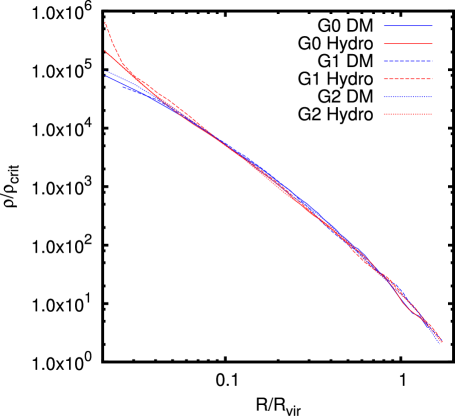
Figure 1: Radial density profile for G0-G2 in the hydro (red lines) and DM (blue lines) simulations.

2.1 Halo finder and merger tree construction

To identify subhaloes in our simulation we use the MPI+OpenMP hybrid ahf halo finder, available freely at http://www.popia.ft.uam.es/AMIGA) and described in detail in Knollmann & Knebe (2009). ahf identifies local over-densities in an adaptively smoothed density field as prospective halo centers. The local potential minima are computed for each of these density peaks and the gravitationally bound particles are determined. Only peaks with at least 50 bound particles are considered to be haloes and retained for further analysis. As subhaloes are embedded within their respective host halo, their own density profile usually shows a characteristic upturn at a radius $r_{t}\mathrel{\hbox to0.0pt{\lower 3.0pt\hbox{$\sim$}\hss}\raise 2.0pt\hbox{$<$}}r_{\rm vir}$, where $r_{\rm vir}$ is the actual (virial) radius of the satellites, were they found in isolation. We use this “truncation radius” $r_{t}$ as the outer edge of the subhaloes and calculate all (sub-)halo properties (i.e. mass) using only the gravitationally bound particles inside $r_{t}$.

As second step we build the merger trees for our galaxies (both hydro and DM), in order to establish the dynamical history of each infalling satellite across cosmic time. For the purpose of constructing an accurate tracking of each simulated (sub)halo, we analyse 40 simulation outputs between $z=2.5$ and $z=0$. We start from the halofinder results at $z=2.5$ and follow these (sub)haloes through cosmic time, adding to the tracking procedure at each snapshot all new haloes that cross our mass threshold. For halo tracking, only dark matter particles are used. We consider two criteria to decide if, when comparing two consecutive snapshots, halo 1 at one output time is the “progenitor” of halo 2 at the subsequent time step: i) more than 50% of the particles in halo 1 that end up in any halo at time step 2 end up in halo 2; ii) more than 50% of the particles in halo 2 come from halo 1.

2.2 ”Twin” matching and orbital parameters

Since we aim to compare the hydrodynamical and pure DM simulations by studying satellite ”twins”, i.e. satellites that formed in both simulations from the same perturbations at the initial time, we perform the following steps to identify these satellite pairs:

1. We use the AHF halo finder to identify a given satellite in the DM simulation at the redshift $\bar{z}$ of interest.

2. We track the position of the satellite DM particles back in time to the initial condition file, in order to determine its original Lagrangian region.

3. We look for DM particles within the set of hydro initial conditions in the same Lagrangian region and map them forward in time to the same redshift $\bar{z}$.

4. Using the satellite catalogue for the hydro simulation we check in which satellite(s) these dm particles end up. We then use the same criteria adopted in the merger tree construction to determine the correct “twin” pair (see Fig. 2).

We have explicitly tested that the exact same results for the satellite mapping follow starting either from the DM or the hydro simulation. Overall we find more than 200 satellites pairs and 76 of them survived down to $z=0$ in both simulations. We will refer to this last subset of satellites as the twin population at redshift zero.

Finally we compute the orbital parameters (apo-center and peri-center distances) for each pair of twin satellites. In order to do that we integrate the satellite orbit in an effective static potential parametrized using the power-law logarithmic slope (PoLLS) model (Cardone et al., 2005):

$$\rho^{\mathrm{PoLLS}}(r)=\rho_{-2}\exp(-\frac{2}{\gamma}\left[\left(\frac{r}{R_{-2}}\right)^{\gamma}-1\right])$$ (1)

where $\rho_{-2}$ is the density at the $R_{-2}$ distance, which is where the profile slope is equal to $-2$ (i.e. the singular isothermal sphere profile) and $\gamma$ is related the central slope of the profile. All these parameters are fitted to match the actual potential in either the DM or hydro simulation. In principle since we have constructed the merger trees it would have been possible to compute the satellite orbital parameters directly from the simulation. On the other hand, given the time sampling of our snapshots we could end up with over/under estimating the peri/apo-centre distances. So we decided to use a frozen potential in order to have a more reliable orbital parameter estimate.

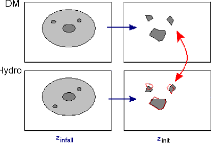
Figure 2: Illustration of satellite mapping scheme.

3 Results

In this section we study how the presence of baryons affects the properties of satellites in our simulations. We include in our analysis only substructures with at least $M_{tot}>10^{8}M_{\odot}$. We combine together the results of G0, G1 and G2 (which give similar results when analyzed individually) and mainly focus on “twin” haloes. This gives us a sample of more than 70 satellite couples at $z=0$. In the following we refer to the dissipationless simulations as pure DM or Nbody, while we use the therm “hydro” for dissipational simulation that include gas and stars.

Figure 3 shows the cumulative radial distribution (for all satellites) in our three galaxies in the two different simulation runs. As first noticed by Macciò et al. (2006) and later confirmed by other studies (e.g. Libeskind et al., 2010; Romano-Díaz et al., 2010) the radial distribution of satellites is clearly more concentrated in hydro simulations (solid red line) than in DM ones (dashed blue line). This trend is partially confirmed when we restrict our analysis to twin satellites as shown in Figure 4, at least in the inner region. We should point out that “twin” satellites are a biased sub sample of the whole satellite population, since, by construction, we restrict ourselves to those satellites that survived until $z=0$ in both simulations. This biased selection explains the difference in the radial distribution profiles of the whole population and of the twin sample in the hydro and DM runs (especially in the external regions).

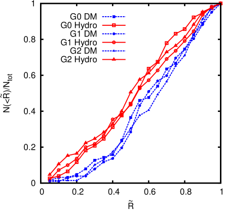
Figure 3: Number density profile of ALL satellites at $z=0$.

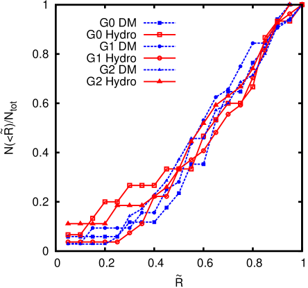
Figure 4: Number density profile of TWIN satellites at $z=0$

.

In order to understand the physical drivers behind the results of Fig. 3 and Fig. 4, we exam individual mass accretion and dynamical histories of all twin couples from $z=1.2$ to the present time. This is the redshift at which the latest major merger happen (namely for the G1 halo), after $z=1.2$ our galaxies have a quiet dynamical history that allows to study in details the satellites properties and orbits Figure 5 shows the evolution with redshift of the distance from the halo centre (upper panel) and the total mass (lower panel) of an hydro subhalo (solid line) and its dm twin (dashed curve). The two satellites enter the virial radius of the main object ($\tilde{R}=1$) at the same time and have similar orbits, ending at $z=0$ at roughly the same distance from the halo centre. In this particular case the mass loss is higher in the hydro case, where the satellite is able to retain only 30% of its mass (50% in the pure DM run). This figure is similar to Figure 8 and 9 of Libeskind et al. (2010), even though the role of DM and hydro are reversed.

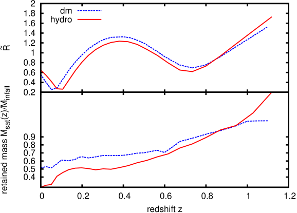
Figure 5: Evolution of radial distance (upper panel) and mass (lower panel) over time for a satellite that lost more mass in the hydrodynamical simulation than in the pure DM one.

.

The behaviour presented in Fig. 5 is rare, however. The majority of satellites have more complicated dynamical histories as shown in Fig. 6. There, it is immediately noticeable that the twins in this case do not enter the virial radius of the parent halo at the same time. The infall time is $z_{infall}=0.93$ in the hydro case and $z_{infall}=1.25$ in the pure DM one. The orbits are moreover very different: in the hydro simulation the satellite has a very large apo-center that brings it outside the virial radius at $z\approx 0.5$ before being re-accreted; this does not happen in the pure DM run. As a consequence, the orbits are practically uncorrelated, and satellites experience different mass loss rates.

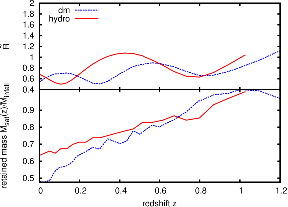
Figure 6: Same as figure 5, but for a satellite that lost less mass in the hydrodynamical run than in the pure DM one.

An interesting feature revealed by Fig. 6 is the difference in the time of accretion between the hydro and DM runs. This is not a peculiar behaviour of the selected satellite, but it is quite a general trend, as shown in Fig. 7. For each twin couple we compute the infall time (defined as the time at which the satellite first crosses the virial radius of the main object) in the hydro and pure DM runs and then we plot the difference in these two times as a function of the infall redshift in the DM case.

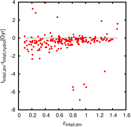
Figure 7: Difference in infall time (e.g. crossing of the virial radius) for twins. $t_{infall}$ is the time measured from the Big-Bang.

Most of the hydro satellites enter the virialized region later than their pure DM counterparts, with an average delay of 0.7 Gyrs. A possible explanation for this delayed accretion might be time evolution in the main halo virial radius. Fig. 9 shows $R_{vir}(z)$ for the hydro and pure DM simulation of the G2 galaxy. (We observe a similar effect for G0 and G1 also.) In both runs the virial radius (in comoving coordinates) grows until $z\approx 0.8$ and then decreases toward $z=0$. Although the DM run shows a larger value of $R_{vir}$ after $z=1$, this difference is very small (about 5%) and cannot explain the results of Fig. 7. This also confirm by figure 8 where we plot the difference of physical distance from the center of the halo for twin couples at the moment the hydro satellite crossed the virial radius. The plot confirms that hydro satellites are substantially farther away compared to their DM counterparts at the time of accretion.

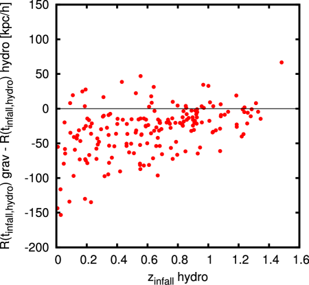
Figure 8: Difference in physical distance from the center of the halo for twins at the time the hydro satellite crossed the virial radius.

An alternative, possible, explanation arises from the point of view of the initial conditions. The hydro and pure DM runs differ only in that a fraction $\Omega_{b}/\Omega_{dm}$ of the total mass in the hydro simulation is represented by gas particles, while these gas particles are converted to dark matter particles for the Nbody run. The lower panel of Fig. 9 shows the mass within a fixed radius of 270 kpc due to baryonic particles (stars + gas) in the hydro run and the same DM-converted particles in the pure DM run. After $z=1$ there, the amount of “converted particles” inside a sphere of 270 kpc exceeds the baryonic mass accumulated within the same region. One possible explanation for this effect is that the pressure in the baryonic hot gas slows down the accretion with respect to the pressure-less ”converted” dark matter component (especially in low density regions where the cooling time of the gas is extremely long). We speculate that the resulting delay in formation within the hydro simulation in this case could explain the delayed accretion of hydro satellites shown in Fig. 7. Nevertheless further studies are needed to confirm our hypothesis.

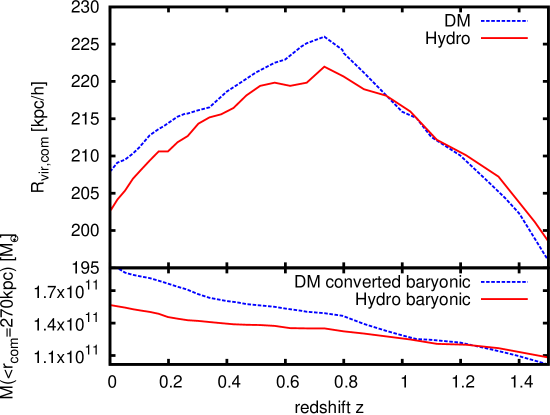
Figure 9: Comparison of evolution of (top) comoving virial radius for G2 and (bottom) mass of (converted) baryonic matter inside sphere of 270 Mpc (comoving)

3.1 Orbital Parameters

The largely different time evolution of $\tilde{R}$ for twin haloes shown in Fig. 6 suggests that the radial position at any fixed redshift is not well-suited for directly comparing the orbits of the “twin” satellites. The peri-centric and apo-centric distances (see Section 2.2), as well as the length of the semi-major axis of the orbit $R_{avg}\equiv(R_{peri}+R_{apo})/2.0$, seem a better choice.

Figure 10 shows the ratio of the average distance ($R_{avg}$) for hydro and pure DM satellites as a function of the average distance in the hydro run. In the pure DM case $\tilde{R}_{avg}\equiv R_{avg}/R_{vir}$ tends to exceed the corresponding value in the hydrodynamical simulations for satellites that are close to the center. In the outer region of the halo the trend is reversed and satellites have a smaller average distance in the pure DM case. This change in the radial behaviour seems to happen around $\tilde{R}_{avg}>0.85$. We will use this (somehow arbitrary) threshold to separate the inner and outer behaviour of our twin subhaloes in the next figures.

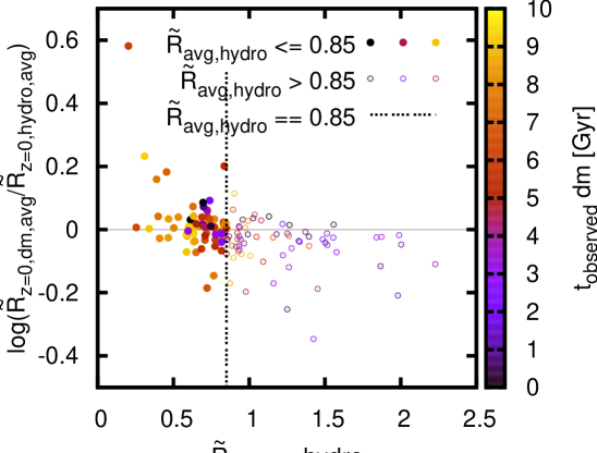
Figure 10: Comparison of average distance of satellite ”twins” at redshift $z=0$. Each couple is color coded according to its DM observation time (i.e. the time at which they are closer than $2\times R_{vir}$ from the main halo center).

In this same plot, twin couples are color coded according to their observation time (i.e. the time at which they are closer than $2\times R_{vir}$ from the main halo center). We find a very interesting correlation between the ratio of $\tilde{R}_{avg}$ in the DM and hydro runs and this observation time. Satellites with low $t_{obs}$ tend to live in the outskirts of the halo and are on average closer to the halo center in the DM run than in the hydro case. In contrast, “old” satellites (i.e. large $t_{obs}$) tend to live in the inner region of the halo and are closer to the halo center in the hydro run than in the pure DM.

This result can be understood in the following way: in the outer region of the halo, dynamical friction is less important, and the distance from the center of a given satellite mainly depends on its accretion time. On the other hand, in the inner regions dynamical friction is stronger in the hydro simulation (due to the central stellar body), dragging satellites toward the center in a more effective way compared to the pure DM case. This picture is confirmed by the comparison between the apo-centre distances for twins shown in Fig. 11. Satellites in the outer region of the halo ($\tilde{R}_{avg,hydro}>0.85$) have a larger apo-center distance in the hydro simulation, while the situation is reversed for satellites further inside the halo.

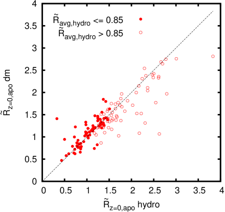
Figure 11: Comparison of apo-centric distance of satellite ”twins” at redshift $z=0$. The apo-centric in computed using a frozen potential modelled according to eq: 1.

3.2 Mass loss

The rate at which mass is removed from a given satellite depends on the balance between the density profile of the satellite and the density profile of the central halo. Libeskind et al. (2010) found that satellites in hydro simulations experience a lower mass loss due to their increased central density. On the other hand Romano-Díaz et al. (2010) found that the central region of hydro galaxies is depleted of satellites at a faster rate than in pure DM simulations, pointing to a faster and stronger mass loss in the hydro case. Figure 12 shows a scatter plot of the retained mass of all twins at $z=0$. Satellites that lose less than 60% of their mass tend to retain more mass in the hydro simulation, consistent with the findings of Libeskind et al. (2010). But satellites that are heavily stripped tend to lose even more mass in the hydro simulation. There is also a clear correlation between the average position of the satellite and the amount of stripping.

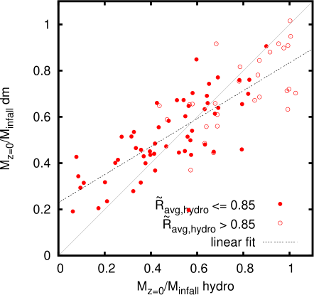
Figure 12: Scatter plot of relative retained mass of twins in pure DM and hydrodynamical simulation (combined results for G0,G1,G2)

This result becomes clearer when comparing the mass loss with the orbital parameters of the satellite ($\tilde{R}_{avg}$), as in Fig. 13. Satellites that live in the external part of the halo tend to be at larger distances from the center and retain more mass in the hydro simulation than in the pure DM one. On the other hand, satellites in the central region are closer to the center and more heavily stripped in the hydro simulation, pointing to a more efficient dynamical friction and tidal stripping (in the central regions) in the hydro simulation, in agreement with the findings of Romano-Díaz et al. (2010).

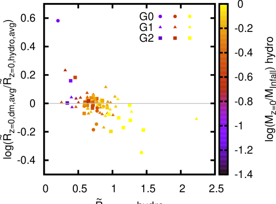
Figure 13: Comparison of the ratio of the average distance in the DM and hydro sim as a function of the average distance in the hydro case. Twins are color coded according to their retained mass in the hydro simulation (combined results for G0,G1,G2).

In Fig. 14 satellites are color-coded according to their total mass (in the hydro simulation) at the time of infall. As expected from dynamical friction theory, more massive satellites are living at $z=0$ closer to center than low mass ones. This implies that satellites with large $M_{infall}$ will be even closer to the center in hydro than in the DM simulations.

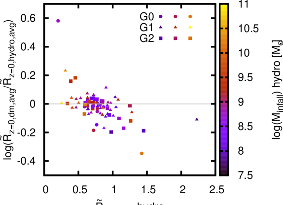
Figure 14: Same as figure 13 but with twins color coded according to their mass at infall time in the hydro simulation (combined results for G0,G1,G2).

Together these results suggest a bimodal picture in which high mass satellite at the time of accretion are closer to the center and more heavily stripped in the hydro simulation than in the pure DM, but the reverse for satellites with low $M_{infall}$, which are on average further way from the center and less stripped in the hydro simulation.

3.3 Danger to the galaxy disk

In this section we assess if and how the different orbital parameters and mass loss rates found for hydro massive satellites influence results previously obtained using pure Nbody simulations (Font et al., 2001; Read et al., 2008; Villalobos & Helmi, 2008; Kazantzidis et al., 2009).

Figure 15 shows a scatter plot of mass versus peri-centric distance for two different twin substructure populations within host galaxies G0-G2. It is equivalent to Fig. 1 of Kazantzidis et al. (2009) and we have used the same values for the scaling quantities $M_{disk}$ and $R_{d}$ as in their work, namely $M_{disk}=3.52\times 10^{10}M_{\odot}$ and $R_{d}=2.82$ kpc.

The first substructure population in Fig. 15 is comprised of all systems that have crossed an infall radius of $r_{\rm inf}=50{\rm kpc}$ from their host halo center since redshift $z=1$. This selection is empirically fixed to identify orbiting satellites that approach the central regions of the host potential and are thus likely to have a significant dynamical impact on the disk structure. We assign masses to the satellites of this group at the simulation output time closest to the time of the first inward crossing of $r_{\rm inf}$, and then use the potential at this same simulation output to compute the orbit peri-center. Note that a single distinct object of this population may be recorded multiple times, as one subhalo may undergo several passes through the central regions of its host with different masses and peri-centers. Many of these satellites suffer substantial mass loss prior to $z=0$.

The second subhalo population consists of all surviving substructures at $z=0$. The dotted line in Fig. 15 encloses an area in the $M_{\rm sub}-r_{\rm peri}$ plane corresponding to satellites more massive than $0.2M_{\rm disk}$ with peri-centers of $r_{\rm peri}\mathrel{\hbox to0.0pt{\lower 3.0pt\hbox{$\sim$}\hss}\raise 2.0pt\hbox{$<$}}20{\rm kpc}$ ($r_{\rm peri}\mathrel{\hbox to0.0pt{\lower 3.0pt\hbox{$\sim$}\hss}\raise 2.0pt\hbox{$<$}}7R_{d}$). Subhaloes within this area should be effective perturbers, and following Kazantzidis et al. (2009) we refer to this area as the “danger zone”. We note, though, that we include this definition here for the purposes of illustration, only.

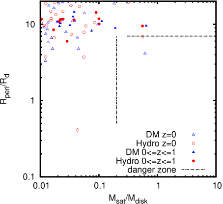
Figure 15: Scatter plot of peri-centric distance versus satellite mass. Filled symbols thereby represent the satellites that cross within a radius of 50 kpc after $z=1$ while unfilled symbols mark the properties of surviving substructures at $z=0$ (twins only)

By this criterion, Figure 15 suggests that satellites in hydro simulation are slightly less dangerous to disk stability than their pure DM counterparts. This can be interpreted on the basis of results shown in the previous sections. While the peri-centric distance does not substantially differ in hydro and DM runs, hydrodynamical satellites face a stronger mass loss. Since the danger for galactic disks is higher the more massive the satellite, this faster mass depletion for hydro satellites implies less dangerous perturbers for galactic disks.

4 Discussion and conclusions

With this work we aim to provide a detailed description of the effects of baryonic physics on the properties of galactic satellites and their evolution with redshift. For this purpose we analyse three different cosmological simulations of galaxy formation, each run twice: once as pure dark matter and another with the addition of gas physics, including gas cooling, star formation and feedback. For each run we create a comprehensive catalogue of the subhalo population at $z=0$ which we trace back in time in order to study mass loss, dynamical friction and evolution of satellite orbital parameters. Within this population we focus on a sub-sample of corresponding DM and hydro satellite pairs (“twins”) and their individual evolutionary histories.

Satellites are found to be more radially concentrated in the hydro simulation than in the pure DM one, confirming earlier results by Macciò et al. (2006). This bias persists also for the twin population, even if slightly less pronounced. When we restrict our analysis to the twin sub-sample we find that hydro satellites tend to enter the virial radius of the parent halo later than the corresponding DM subhaloes, with an average delay of 0.7 Gyrs. This difference cannot be ascribed to a difference in the evolution of $R_{vir}$ in the two simulations, and we speculate that it is instead related to the pressure support of the hot gas that acts against collapse, which, in low density regions, is not counterbalanced by cooling. Nevertheless further studies are need to confirm our hypothesis.

Given the delay in the accretion time, the orbits of twin satellites are often weakly correlated. As a consequence, we find that the radial position at a given redshift is not sufficient to describe the satellite orbit. For this reason we define an average radius $R_{avg}$ for each satellite equal to the median between the apocenter and pericenter distances of the satellite orbit, where these last two quantities are obtained by integrating each satellite orbit in a fixed potential resembling that of the halo. We find that the ratio of the average positions in the hydro and DM cases measured at redshift zero correlates with the accretion time of the satellite and its mass at that time. Moreover, we find that both the absolute mass loss experienced by the satellite and the difference in mass loss in the hydro and DM simulations also correlate with the subhalo average distance at $z=0$.

We arrive at a final picture in which more massive satellites at the time of accretion are closer to the center and more heavily stripped in the hydro simulation than in the pure DM. The situation is reversed for satellites with low $M_{infall}$ that are on average further way from the center and less stripped in the hydro simulation.

This bimodality can be understood in the following way: in the outer region of the halo, dynamical friction is less important, and the distance from the center of a given satellite mainly depends on its accretion time. Since hydro satellites tend to be accreted later, they experience lower dynamical friction and mass stripping than their pure DM counterparts. In the inner regions, on the other hand, dynamical friction is stronger in the hydro simulation (due to the central stellar body) and drags satellites toward the center in a more effective way compared to the pure DM case. Although the baryons provide a substantial glue to the subhaloes, the main halo exhibits the same trend. This assures a more efficient tidal stripping of the hydro subhalo population, resulting in a larger mass loss.

During the making of this work, two other groups, i.e. Libeskind et al. (2010) and Romano-Díaz et al. (2010), independently pursued the same subject. Both studies compared hydro and pure DM simulations using an approach similar to ours, including a focus on corresponding pairs of satellites. The publication of Libeskind et al. mainly considers the radial distribution of the satellites and a comparison of the retained masses. Like us, they find a difference in the orbits of twins. But in contrast to our approach, Libeskind et al. (2010) use the statistics of the radial orbit position, rather then, e.g. determine the orbital parameters and the resulting average distance as we do. They find a larger mass loss for the satellite in the pure DM simulation and interpret this as a sign of the expected higher stability of the hydrodynamical satellite, which our results are only able to confirm in the external region of the halo. Romano-Díaz et al. (2010) on the other hand, find an increased mass loss for the hydrodynamical satellite in the central region of the halo, in accordance with our results. They are also able to detect the final disruption of a satellite, and have shown that the life expectancy of the satellites in the hydrodynamical simulation is indeed shorter than in the pure DM simulation, as our findings suggest.

We extend this result further in the last part of our study by investigating the possible impact of different orbital parameters and mass loss in hydrodynamical simulations, i.e. whether this translates into an increase, or a reduction, in the danger that these satellites pose for the stability of a possible stellar disk at the center of the parent halo (e.g. Kazantzidis et al., 2009; Moster et al., 2010). While the peri-centric distance does not substantially differ in hydro and DM runs, hydrodynamical satellites in the central region face a stronger mass loss. As the danger for galactic disks is linked to the mass of the satellite, this faster mass depletion for hydro satellites leads to less dangerous perturbers for galactic disks, possibly easing the problem of the existence of thin disks in a Cold Dark Matter Universe.

We emphasize, though, that, as correctly pointed out by Romano-Díaz et al. (2010), the effects of baryonic cooling in the center of dark matter (sub)haloes can be altered (if not reversed) for a more efficient feedback from stellar evolution and possibly central super-massive black holes, which will expel baryons from the center and decrease the central concentration of the prime halo (e.g. El-Zant et al., 2004; Mashchenko et al., 2006; Governato et al., 2010).

At this time, the direct comparison of our study of galactic satellites with observations is not possible. The Sloan Digital Sky Survey, which greatly contributed to the discovery and study of several Milky Way satellites (e.g. Koposov et al., 2008; de Jong et al., 2010), covers only a single patch of the sky. Future surveys like Pan-Starrs, which will provide a more comprehensive map of the (northern) sky, promise a better understanding of the properties and spatial distribution of satellite galaxies orbiting around the Milky Way.

References

- Bailin et al. (2005) Bailin J., Kawata D., Gibson B. K., Steinmetz M., Navarro J. F., Brook C. B., Gill S. P. D., Ibata R. A., Knebe A., Lewis G. F., Okamoto T., 2005, ApJL, 627, L17
- Cardone et al. (2005) Cardone V. F., Piedipalumbo E., Tortora C., 2005, MNRAS, 358, 1325
- de Jong et al. (2010) de Jong J. T. A., Martin N. F., Rix H., Smith K. W., Jin S., Macciò A. V., 2010, ApJ, 710, 1664
- De Lucia et al. (2004) De Lucia G., Kauffmann G., Springel V., White S. D. M., Lanzoni B., Stoehr F., Tormen G., Yoshida N., 2004, MNRAS, 348, 333
- Diemand et al. (2007) Diemand J., Kuhlen M., Madau P., 2007, ApJ, 667, 859
- Duffy et al. (2010) Duffy A. R., Schaye J., Kay S. T., Dalla Vecchia C., Battye R. A., Booth C. M., 2010, MNRAS, 405, 2161
- El-Zant et al. (2004) El-Zant A. A., Hoffman Y., Primack J., Combes F., Shlosman I., 2004, ApJL, 607, L75
- Font et al. (2001) Font A. S., Navarro J. F., Stadel J., Quinn T., 2001, ApJL, 563, L1
- Gao et al. (2004) Gao L., White S. D. M., Jenkins A., Stoehr F., Springel V., 2004, MNRAS, 355, 819
- Gnedin et al. (2004) Gnedin O. Y., Kravtsov A. V., Klypin A. A., Nagai D., 2004, ApJ, 616, 16
- Governato et al. (2010) Governato F., Brook C., Mayer L., Brooks A., Rhee G., Wadsley J., Jonsson P., Willman B., Stinson G., Quinn T., Madau P., 2010, Nature, 463, 203
- Governato et al. (2007) Governato F., Willman B., Mayer L., Brooks A., Stinson G., Valenzuela O., Wadsley J., Quinn T., 2007, MNRAS, 374, 1479
- Haardt & Madau (1996) Haardt F., Madau P., 1996, APJ, 461, 20
- Katz (1992) Katz N., 1992, ApJ, 391, 502
- Kazantzidis et al. (2009) Kazantzidis S., Zentner A. R., Kravtsov A. V., Bullock J. S., Debattista V. P., 2009, ApJ, 700, 1896
- Kennicutt (1998) Kennicutt Jr. R. C., 1998, ApJ, 498, 541
- Klypin et al. (1999) Klypin A., Kravtsov A. V., Valenzuela O., Prada F., 1999, ApJ, 522, 82
- Knebe et al. (2010) Knebe A., Libeskind N. I., Knollmann S. R., Martinez-Vaquero L. A., Yepes G., Gottloeber S., Hoffman Y., 2010, ArXiv e-prints
- Knollmann & Knebe (2009) Knollmann S. R., Knebe A., 2009, APJS, 182, 608
- Komatsu et al. (2009) Komatsu E., Dunkley J., Nolta M. R., Bennett C. L., Gold B., Hinshaw G., Jarosik N., Larson D., Limon M., Page L., Spergel D. N., Halpern M., Hill R. S., Kogut A., Meyer S. S., Tucker G. S., Weiland J. L., Wollack E., Wright E. L., 2009, ApJS, 180, 330
- Koposov et al. (2008) Koposov S., Belokurov V., Evans N. W., Hewett P. C., Irwin M. J., Gilmore G., Zucker D. B., Rix H., Fellhauer M., Bell E. F., Glushkova E. V., 2008, ApJ, 686, 279
- Kravtsov et al. (2004) Kravtsov A. V., Berlind A. A., Wechsler R. H., Klypin A. A., Gottlöber S., Allgood B., Primack J. R., 2004, ApJ, 609, 35
- Libeskind et al. (2010) Libeskind N. I., Yepes G., Knebe A., Gottlöber S., Hoffman Y., Knollmann S. R., 2010, MNRAS, 401, 1889
- Macciò et al. (2010) Macciò A. V., Kang X., Fontanot F., Somerville R. S., Koposov S., Monaco P., 2010, MNRAS, 402, 1995
- Macciò et al. (2006) Macciò A. V., Moore B., Stadel J., Diemand J., 2006, MNRAS, 366, 1529
- Mashchenko et al. (2006) Mashchenko S., Couchman H. M. P., Wadsley J., 2006, Nature, 442, 539
- Moore et al. (1999) Moore B., Ghigna S., Governato F., Lake G., Quinn T., Stadel J., Tozzi P., 1999, ApJL, 524, L19
- Moster et al. (2010) Moster B. P., Macciò A. V., Somerville R. S., Johansson P. H., Naab T., 2010, MNRAS, 403, 1009
- Nagai & Kravtsov (2005) Nagai D., Kravtsov A. V., 2005, ApJ, 618, 557
- Quinn et al. (1993) Quinn P. J., Hernquist L., Fullagar D. P., 1993, ApJ, 403, 74
- Read et al. (2008) Read J. I., Lake G., Agertz O., Debattista V. P., 2008, MNRAS, 389, 1041
- Reed et al. (2005) Reed D., Governato F., Quinn T., Gardner J., Stadel J., Lake G., 2005, MNRAS, 359, 1537
- Romano-Díaz et al. (2009) Romano-Díaz E., Shlosman I., Heller C., Hoffman Y., 2009, ApJ, 702, 1250
- Romano-Díaz et al. (2010) Romano-Díaz E., Shlosman I., Heller C., Hoffman Y., 2010, ApJ, 716, 1095
- Sommer-Larsen & Limousin (2010) Sommer-Larsen J., Limousin M., 2010, MNRAS, p. 1332
- Springel et al. (2008) Springel V., Wang J., Vogelsberger M., Ludlow A., Jenkins A., Helmi A., Navarro J. F., Frenk C. S., White S. D. M., 2008, MNRAS, 391, 1685
- Springel et al. (2001) Springel V., Yoshida N., White S. D. M., 2001, New Astronomy, 6, 79
- Stadel (2001) Stadel J., 2001, PhD thesis, University of Washington
- Stinson et al. (2006) Stinson G., Seth A., Katz N., Wadsley J., Governato F., Quinn T., 2006, MNRAS, 373, 1074
- Toth & Ostriker (1992) Toth G., Ostriker J. P., 1992, ApJ, 389, 5
- Velazquez & White (1999) Velazquez H., White S. D. M., 1999, MNRAS, 304, 254
- Villalobos & Helmi (2008) Villalobos Á., Helmi A., 2008, MNRAS, 391, 1806
- Wadsley et al. (2004) Wadsley J. W., Stadel J., Quinn T., 2004, New Astronomy, 9, 137
- Weinberg et al. (2008) Weinberg S. H., Colombi S., Davé R., Katz N., 2008, ApJ, 678, 6
- White & Rees (1978) White S. D. M., Rees M. J., 1978, MNRAS, 183, 341
- Zentner et al. (2005) Zentner A. R., Kravtsov A. V., Gnedin O. Y., Klypin A. A., 2005, ApJ, 629, 219