Charge-starved, relativistic jets and blazar variability

Abstract

High energy emission from blazars is thought to arise in a relativistic jet launched by a supermassive black hole. The emission site must be far from the hole and the jet relativistic, in order to avoid absorption of the photons. In extreme cases, rapid variability of the emission suggests that structures of length-scale smaller than the gravitational radius of the central black hole are imprinted on the jet as it is launched, and modulate the radiation released after it has been accelerated to high Lorentz factor. We propose a mechanism which can account for the acceleration of the jet, and for the rapid variability of the radiation, based on the propagation characteristics of large-amplitude waves in charge-starved, polar jets. Using a two-fluid ($e^{\pm}$) description, we find the outflows exhibit a delayed acceleration phase, that starts when the inertia associated with the wave currents becomes important. The fluids propagate with the wave at approximately the sonic speed, corresponding to a bulk Lorentz factor $\gamma\approx 10^{4}\Delta t_{100}^{1/3}\kappa_{r_{\rm g}}^{-1/3}L_{46}^{1/6}M_{9}^{-1/3}$ out to radius $r_{1}\approx\Delta t_{100}^{1/3}\kappa_{r_{\rm g}}^{2/3}L_{46}^{1/6}M_{9}^{2/3}\,\textrm{pc}$, after which the Lorentz factor accelerates as $\gamma\propto r$. ($\Delta t_{100}$ is the variability time in units of $100\,$s, $\kappa_{r_{\rm g}}$ the pair multiplicity at one gravitational radius, $L_{46}$ the “$4\pi$-luminosity” of the jet in units of $10^{46}\,\textrm{erg/s}$, and $M_{9}$ the black-hole mass in units of $10^{9}\,\mbox{M${}_{\odot}$}$.) The time-structure imprinted on the jet at launch modulates photons produced by the accelerating jet provided $\kappa_{r_{\rm g}}<14\,\Delta t_{100}L_{46}^{1/8}M_{9}^{-1}$, suggesting that very rapid variability is confined to sources in which the electromagnetic cascade in the black-hole magnetosphere is not prolific.

1. Introduction

Observations by the H.E.S.S. collaboration of TeV gamma-ray emission from the blazar PKS 2155-304 reveal very rapid variability (Aharonian et al. 2007; HESS Collaboration et al. 2010), at very high flux levels. In the most extreme flare, variations on a timescale of a few hundred seconds at a flux level corresponding to an isotropic luminosity of $10^{46}\,\textrm{erg/s}$ were measured. If, as expected, the mass $M$ of the central black hole is $2\times 10^{9}\,\mbox{M${}_{\odot}$}$, these observations imply structure in the jet that is roughly one hundred times smaller than the gravitational radius $r_{\rm g}=GM/c^{2}$ (Begelman et al. 2008). Though this is the most extreme example, several other blazars exhibit very rapid variability in GeV and TeV gamma-rays (e.g., Albert et al. 2007; Ackermann et al. 2010), which it is proving difficult to accommodate in the standard synchrotron-self-Compton picture, mainly because of the very high Lorentz factor and low magnetisation required of the jet (Levinson 2007; Boutelier et al. 2008; Graff et al. 2008; Katarzyński et al. 2008; Kusunose & Takahara 2008; Mastichiadis & Moraitis 2008; Neronov et al. 2008; Ghisellini et al. 2009; Giannios et al. 2009; Paggi et al. 2009; Tammi & Duffy 2009; Rieger & Volpe 2010; Nalewajko et al. 2010).

In the framework of ideal MHD, radial (uncollimated) relativistic jets do not accelerate after they pass through the fast magnetosonic point. Collimation, however, requires special boundary conditions (Lyubarsky 2009, 2010). It is, therefore, difficult to envisage the production of a jet with high Lorentz factor and low magnetisation. An isolated, impulsive, ejection event in an ideal MHD flow is able to circumvent this problem (Granot et al. 2010), but, in a fluctuating jet, dispersion filters out the small timescale structure, and limits the acceleration (Levinson 2010a). It appears, therefore, that it may be necessary to go beyond the ideal MHD approximation in order to understand the observations of very rapid variability in blazars.

Non-ideal MHD effects can become important when plasma is charge-starved: If the number density of charged particles is limited, this places a maximum on the absolute value of the charge density, which can, for example, result in the inability of the plasma to screen out the component of the electric field parallel to the magnetic field. Charge starvation also places an upper limit on the available current density. As this limit is approached, the relative drift-speed of the charged components becomes relativistic, and their associated inertia begins to contribute to the fluid stress-energy tensor. This situation might plausibly arise in a black-hole magnetosphere, because axisymmetric, general-relativistic, MHD simulations of jets launched by accreting, rotating black holes (De Villiers & Hawley 2003; McKinney & Gammie 2004) reveal a conical region around the rotation axis into which the accreting plasma does not penetrate. As in a pulsar magnetosphere, the matter density in this region is likely to be determined not by accretion, but by the rate at which electron-positron pairs are created in the strong electromagnetic fields that penetrate it (Goldreich & Julian 1969; Blandford & Znajek 1977; Levinson 2000). If an outflow results, the density of pairs decreases, and, far from the hole, non-MHD effects connected with particle inertia can become important.

In the case of an axisymmetric, force-free magnetosphere, it is known that plasma is ejected, carrying off energy mainly in the form of Poynting flux via the “Blandford-Znajek” mechanism. On the axis itself, the energy flux vanishes, so that the polar regions of the jet do not dominate the overall energetics. However, observations of rapid variability suggest that axisymmetry may not be a good approximation, since they imply small-scale structure in the black-hole magnetosphere. Simulations in which the black-hole spin and the asymptotic magnetic field are misaligned find a Poynting flux comparable to the Blandford-Znajek value (Palenzuela et al. 2010), making it plausible that also more complex non-axisymmetric field structures can power a substantial, magnetically dominated, polar jet.

In the following, we develop this idea by examining the propagation characteristics of nonlinear electromagnetic waves above the polar regions of a rotating black hole. Using a model consisting of cold electron and positron fluids, we show that a circularly polarised magnetic shear propagates radially outwards at roughly the fast magnetosonic speed until it reaches the point where the ideal MHD description loses its validity. In (non-ideal) MHD language, this happens when the inertia of the plasma particles begins to affect the conductivity, i.e., when the drift speeds implied by the plasma current become relativistic (Melatos & Melrose 1996; Meier 2004). This can occur at a large distance from the black hole, depending on the density of injected pairs. The wave then goes through a phase of delayed acceleration in which it converts Poynting flux into kinetic energy flux. If particles radiate gamma-rays in the acceleration zone, then, despite the large spatial extent of the source, the spatio-temporal structure of the shear wave, that is imprinted on it close to the black hole, modulates the radiation, provided the mass-loading of the jet is sufficiently small.

In section 2 we discuss the parameters used to specify the physical conditions in the jet. The two-fluid jet model is presented in section 3. First, the nonlinear plane-wave solution representing a magnetic shear is derived, then radial propagation in spherical geometry is discussed. It is shown in the Appendix that general relativistic effects drop out in the short-wavelength approximation ($c/\omega\ll r$) when the Kerr metric is used. The application to blazar variability is discussed in section 4, and our conclusions summarised in 5.

2. Jet parameters

Consider a radial outflow consisting of an electron-positron plasma emerging from the polar regions of the magnetosphere of a rotating black hole, and denote by $L$ and $\dot{M}$ the total luminosity and mass-flux carried in a solid opening angle $\Omega_{\rm s}$. The physical conditions in the flow can be specified via three dimensionless parameters:

1. The nonlinearity or strength parameter $a$ is a dimensionless measure of the energy-flux density. For a circularly polarized vacuum electromagnetic wave of frequency $\omega/2\pi$ and electric field $E$, the strength parameter is conventionally defined as $a=eE/(mc\omega)$, and measures the Lorentz factor that an electron would achieve if it were accelerated from rest over a distance of $\left(2\pi\right)^{-1}$ times one wavelength in the field $E$. Assuming radial propagation, the corresponding luminosity is

   $$L = \frac{m^{2}c^{3}\omega^{2}a^{2}\Omega_{\rm s}r^{2}}{4\pi e^{2}}\enspace,$$ (1)

   and we use this expression to define $a$ for a general (non-vacuum) wave. In the absence of radiation losses, $a\propto r^{-1}$, and is determined by specifying its value at some fiducial radius. For this we chose $r_{0}=c/\omega$, although our treatment is, of course, valid only for $r\gg r_{0}$ and we certainly do not expect radial flow to extend to such small radii. With this choice, $a_{0}$ is independent of $\omega$:

   $$a = a_{0}\left(r_{0}/r\right)$$ (2)

   $$a_{0} = \left[\frac{4\pi e^{2}L}{m^{2}c^{5}\Omega_{\rm s}}\right]^{1/2}$$ (3)

   $$= 3.4\times 10^{14}L_{46}^{1/2}\enspace,$$

   where $L_{46}=\left(4\pi/\Omega_{\rm s}\right)L/\left(10^{46}\,\textrm{erg/s}\right)$ is the “isotropic” or “$4\pi$” luminosity of the jet, scaled appropriately. The energy radiated per unit solid angle by a jet is directly measurable if the distance to the object is known. For the rapidly variable gamma-ray flare of PKS 2155-304, it corresponds to an isotropic luminosity of roughly $10^{46}\,\textrm{erg/s}$, so that, for this object, $L_{46}\gtrsim 1$.

2. The mass-loading of the wind is conventionally described by the $\mu$-parameter introduced by Michel (1969):

   $$\mu = L/\dot{M}c^{2}\enspace.$$ (4)

   In the case of an electron-positron jet, $\mu$ denotes the Lorentz factor each particle would have if the entire luminosity was carried by a cold, unmagnetised flow. It is constant in those parts of the jet in which pair creation and radiation losses can be neglected.

3. The magnetisation parameter $\sigma$ describes the ratio of the energy flux carried by electromagnetic fields to that carried by particles. For monoenergetic electrons and positrons of Lorentz factor $\gamma$,

   $$\sigma = \left(\mu/\gamma\right)-1\enspace.$$ (5)

   In a cold, non-accelerating, ideal MHD flow, $\sigma$ is constant (assuming pair creation and radiation losses are negligible). However, as we show below, $\sigma$ is not constant in charge-starved jets, even in the absence of dissipation. For this reason, we specify its value at the “launching” radius, inside of which the ideal MHD approximation is assumed to hold, and denote this quantity by $\sigma_{0}$, even though the region of constant $\sigma$ is unlikely to extend to radii as small as $r\sim c/\omega$. The particle Lorentz factor at the launching point is then

   $$\gamma_{0} = \mu/\left(\sigma_{0}+1\right)\enspace.$$ (6)

The mass-loading parameter $\mu$ is determined by the physics of the pair-production cascade close to the black hole. A more intuitive measure, therefore, is the pair multiplicity $\kappa$, which relates the pair (proper) number density $n_{\pm}$ to the number density of electrons (or positrons) needed to screen out the (magnetic-)field-aligned component of the rotation-induced electric field. Adopting the definition conventionally used in pulsar physics, but replacing the angular velocity of the neutron star by $c/r_{\rm g}$ gives (e.g., Lyubarsky & Kirk 2001)

$$\kappa = \gamma_{\pm}n_{\pm}\left(\frac{B}{2\pi er_{\rm g}}\right)^{-1}\enspace,$$ (7)

where $\gamma_{\pm}$ is the Lorentz factor of the fluids. In the inner regions of the flows we consider, where $\sigma=\sigma_{0}\gg 1$, the fluids move non-relativistically in the wave frame, so that $\kappa\approx a/\left(4\mu\right)$. Thus, in the absence of radiation losses and pair production, $\kappa\propto r^{-1}$ in this region. Physically, it is the value of $\kappa$ at the outer boundary of the pair-production region that is most relevant. This is thought to be close to the black hole, but its precise location is unknown. In the following, therefore, we specify $\kappa$ by its value $\kappa_{r_{\rm g}}$ at $r=r_{\rm g}$:

$$\kappa_{r_{\rm g}} \approx \frac{a_{0}}{4\mu}\left(\frac{c}{\omega r_{\rm g}}\right)\enspace.$$ (8)

3. The two-fluid model

The simplest model of an electron-positron plasma that captures the physics connected with the finite inertia of the charge-carriers is that of two cold, oppositely charged fluids (denoted by suffices $-$ and $+$). We adopt this model, embed it in a Kerr metric, following Khanna (1998) and Koide (2009), and look for large-amplitude waves propagating in the radial direction in Boyer-Lindquist coordinates. To keep the analysis tractable, only transverse waves with vanishing phase-averaged components of the electric and magnetic fields are treated. In this case, since $\nabla\cdot\bm{E}=0$, the number density is the same for each fluid. We further assume the wave carries no radial current, so that the radial fluid velocities also equal each other: $v_{\hat{r}+}=v_{\hat{r}-}=v_{\hat{r}}$, and restrict the treatment to waves in which the meridional and azimuthal fluid velocities are equal in magnitude but of opposite sign: $v_{\hat{\theta}+}=-v_{\hat{\theta}-}$, $v_{\hat{\phi}+}=-v_{\hat{\phi}-}$. It follows that the fluids have the same Lorentz factor: $\gamma_{+}=\gamma_{-}=\gamma=c/\left(c^{2}-v_{\hat{r}}^{2}-v_{\hat{\theta}+}^{2}-v_{\hat{\phi}+}^{2}\right)^{1/2}$, and the same radial component of the four-velocity, which we write as a dimensionless momentum: ${p_{\|}}=v_{\hat{r}}\gamma/c$. Circularly polarised waves are likely to be the most important in the polar regions of a rotating black hole, and these are best treated by introducing complex quantities to describe the transverse components of the fluid momenta: ${p_{\bot}}=\left(v_{\hat{\theta}+}+iv_{\hat{\phi}+}\right)\gamma/c$ ($=-\left(v_{\hat{\theta}-}+iv_{\hat{\phi}-}\right)\gamma/c$) and the electric and magnetic fields: $E=E_{\hat{\theta}}+iE_{\hat{\phi}}$, $B=B_{\hat{\theta}}+iB_{\hat{\phi}}$. In Appendix A we derive the continuity equation, the equations of motion of the fluids and the two relevant Maxwell equations (Faraday’s law and Ampère’s law) in the small-wavelength approximation, $r\gg c/\omega$, starting from the formulation given by Khanna (1998). In the lowest order, we search for large-amplitude plane-wave solutions using the approach introduced by Akhiezer & Polovin (1956).

3.1. Nonlinear waves

Expressing all quantities in terms of the phase $\phi$ defined in (A8), the continuity equation (A12) and Faraday’s law (A13) integrate immediately to give

$$n\Delta =$$ constant (9)

$$B = iE/\beta_{\rm w}\enspace,$$ (10)

where $\Delta=\gamma-\left({p_{\|}}/\beta_{\rm w}\right)$, and $c\beta_{\rm w}$ is the phase speed of the wave. The equations of motion to this order, (A15) and (A16), are

$$\omega\Delta\frac{\textrm{d}{p_{\|}}}{\textrm{d}\phi} = -\frac{e}{mc}\textrm{Im}\left({p_{\bot}}B^{*}\right)$$ (11)

$$\omega\Delta\frac{\textrm{d}{p_{\bot}}}{\textrm{d}\phi} = -i\frac{eB}{mc}\Delta\enspace.$$ (12)

Solutions to these equations can be found with superluminal phase speed, $\beta_{\rm w}>1$, but these waves do not propagate close to the black hole (Kirk 2010). Here, we concentrate on subluminal waves, for which the condition $\Delta=0$ holds. Physically, this means that the particles are in resonance with the wave, i.e., the radial components of the fluid velocities equal the phase velocity of the wave. In this case (9) shows that the phase dependence of the density is arbitrary, (12) is trivially satisfied, and (11) requires that the transverse components of the fluid velocities are parallel to the magnetic field: $\textrm{Im}\left({p_{\bot}}B^{*}\right)=0$. Thus, the plasma current is directed along the magnetic field and, to this order, the forces exerted on the fluids by the fields vanish. Finally, the current and magnetic field are linked by Ampere’s equation, which, to this order, reads

$$\frac{\partial B}{\partial\phi} = \frac{8\pi inec{p_{\bot}}\beta_{\rm w}}{\omega\left(1-\beta_{\rm w}^{2}\right)}\enspace.$$ (13)

Combined with (11) this implies that the magnitude of the magnetic field is phase-independent. Viewed from a frame that moves radially with speed $\beta_{\rm w}$, the electric field vanishes, and the wave is simply a static magnetic field of constant magnitude whose direction rotates through $2\pi$ radians over one wavelength. At each point, the current and, hence ${p_{\bot}}$, is parallel to the magnetic field to zeroth order. The rate at which the $B$-vector rotates is arbitrary, being determined by the dependence of the fluid density $n$ on phase. In the following, we select the simplest case, where $n$, $\left|B\right|^{2}$ and $\left|{p_{\bot}}\right|^{2}$ are all constant and the wave is a monochromatic magnetic shear: $B\propto{p_{\bot}}\propto\textrm{e}^{\pm i\phi}$.

3.2. Radial evolution of a magnetic shear

The slow evolution of the subluminal magnetic shear wave as it propagates outwards at $r\gg r_{\rm g}$ is governed by the first-order equations in the expansion in $\epsilon\sim c/\left(\omega r\right)$, as derived in Appendix A. Making obvious simplifications to the notation, these are the continuity equation (A33):

$${p_{\|}} = \mu\hat{\omega}^{2}/R^{2}\enspace,$$ (14)

the equation of energy flux conservation:

$$\mu = \gamma(1+\sigma)$$ (15)

and the radial momentum equation

$$\frac{d\nu}{dR}=\frac{R|{p_{\bot}}|^{2}}{\mu\hat{\omega}^{2}}\enspace,$$ (16)

where the momentum-flux density per unit mass-flux

$$\nu = {p_{\|}}\left(1+\frac{1+\beta_{\rm w}^{2}}{2\beta_{\rm w}^{2}}\sigma\right)$$ (17)

and $\hat{\omega}=\omega/\omega_{\rm p}$ (with the plasma frequency defined using the proper fluid density: $\omega_{\rm p}^{2}=8\pi ne^{2}/m$), $R=\left(\omega r/c\right)\left(\mu/a_{0}\right)$ is the radius in units of the critical radius, inside of which the superluminal modes do not propagate (Kirk 2010). Note that in a non-monochromatic wave, the quantities ${p_{\|}}$, $\hat{\omega}$, $\sigma$ and $\gamma$ are replaced in these equations by their phase-averages.

According to (13), $\sigma$, as defined in (A32) is related to the fluid momentum components through

$$\sigma = \frac{\beta_{\rm w}^{4}\gamma_{\rm w}^{4}\left|{p_{\bot}}\right|^{2}}{\hat{\omega}^{2}{p_{\|}}^{2}}\enspace,$$ (18)

where $\gamma_{\rm w}=\left(1-\beta_{\rm w}^{2}\right)^{-1/2}$. The condition that the wave velocity equals the radial component of the fluid velocity, $\Delta=0$, implies

$$\gamma_{\rm w}^{2} = \gamma^{2}/\left(1+\left|{p_{\bot}}\right|^{2}\right)\enspace.$$ (19)

The five equations (14)–(19), together with the definition $\gamma=\left(1+{p_{\|}}^{2}+\left|{p_{\bot}}\right|^{2}\right)^{1/2}$, determine the radial dependence of the six unknown wave variables $\gamma_{\rm w}$, $\gamma$, ${p_{\|}}$, $\left|{p_{\bot}}\right|$, $\hat{\omega}$, and $\sigma$. It is straightforward to reduce these to a first-order ordinary differential equation for ${p_{\bot}}(\gamma_{\rm w})$, for example. Solutions extend from $R=0$ to $R=\infty$ provided they are launched at super-magnetosonic speed: $\sigma=(\mu/\gamma)-1<\mu^{2/3}$. At $R\rightarrow 0$, $\left|{p_{\bot}}\right|\rightarrow 0$ and $\gamma\rightarrow\gamma_{\rm w}$. whereas at $R\rightarrow\infty$, $\sigma\rightarrow 0$ and $\gamma\rightarrow\mu$, so that the wave converts all of the Poynting flux to kinetic energy at large radius.

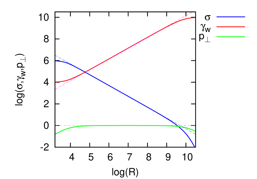
Figure 1.— The magnetisation parameter $\sigma$, transverse fluid momentum ${p_{\bot}}$ and Lorentz factor of the wave, $\gamma_{\rm w}$, as functions of the dimensionless radius $R=\mu r\omega/\left(a_{0}c\right)$, for $\sigma_{0}=10^{6}$ and $\mu=10^{10}$. The approximate solutions given in Eq. (22) are also shown.

The radial dependence of the wave goes through three phases. At small $R$, $\left|{p_{\bot}}\right|\ll 1$ and the wave is essentially a cold MHD structure in which the inertia associated with the current is negligible. There is no acceleration of either the wave speed or the fluids in this regime, and the magnetisation parameter $\sigma$ remains constant at its initial value $\sigma_{0}$. Assuming $\sigma_{0}\gg 1$, this region is restricted to $R\ll\mu/\sigma_{0}$. At intermediate radii, one readily finds an approximate solution:

$$\begin{array}[]{r@{\,\approx\,}l@{\qquad}r@{\,\approx\,}l}{p_{\bot}}&1&\sigma&\mu/\left(2R\right)\\ \gamma&2R&\gamma_{\rm w}&\gamma/\sqrt{2}\enspace,\end{array}$$ (22)

valid in the range

$$\mu/\sigma_{0}\ll R\ll\mu\enspace.$$ (23)

Finally, at large radius, $R\gg\mu$, only kinetic energy remains: $\gamma\approx\gamma_{\rm w}\approx\mu$, $\left|{p_{\bot}}\right|\ll 1$. This behaviour is illustrated in Fig. 1.

4. Application to blazar variability

The locations of the three phases of wave propagation illustrated in Fig. 1 depend on the parameters $a_{0}$, $\mu$ (or $\kappa_{r_{\rm g}}$), $\sigma_{0}$ and $\omega$. As discussed in Sect. 2, it is possible to infer values for $a_{0}$ and $\omega$ directly from the observed flux and variability timescale. Another parameter may be eliminated by fixing the wave speed at its launching point. A very slow, sub-magnetosonic outflow can be described by the force-free MHD equations, and would accelerate as $\gamma\propto r$ (Buckley 1977), until it approached the sonic speed, where $\gamma_{0}\approx\sigma_{0}^{1/2}\approx\mu^{1/3}$. On the other hand, all waves launched at super-magnetosonic speeds ($\sigma_{0}<\mu^{2/3}$) behave similarly, as described in Sect. 3.2, with the acceleration phase moving out to larger radius as the initial magnetisation decreases. It suffices, therefore, to analyse the case of mildly supersonic launch: $\sigma_{0}\approx\mu^{2/3}$, corresponding to the maximum magnetisation of a supersonic flow.

However, the uncertainty associated with the unknown mass-loading of the flow can be removed only by modelling the pair cascade. Leaving this quantity as a free parameter, the radius $r_{\rm acc}$ at which acceleration begins, corresponding to $R\approx\mu/\sigma_{0}$, is

$$r_{\rm acc} \approx r_{\rm g}a_{0}^{1/3}\kappa_{r_{\rm g}}^{2/3}\left(\omega r_{\rm g}/c\right)^{-1/3}$$ (24)

$$= 1.2\,\Delta t_{100}^{1/3}\kappa_{r_{\rm g}}^{2/3}L_{46}^{1/6}M_{9}^{2/3}\,\textrm{pc}\enspace,$$

where we define the variation timescale in units of $100\,$s to be $\Delta_{100}=\left(2\pi/\omega\right)/\left(100\,\textrm{s}\right)$, and write the mass of the black hole as $M=M_{9}\times 10^{9}\,\mbox{M${}_{\odot}$}$. For $r<r_{\rm acc}$ the Lorentz factor of the flow remains constant at roughly the sonic speed:

$$\gamma_{0} \approx 6.5\times 10^{3}\Delta t_{100}^{1/3}\kappa_{r_{\rm g}}^{-1/3}L_{46}^{1/6}M_{9}^{-1/3}$$ (25)

and, for $r>r_{\rm acc}$, the Lorentz factors increase linearly with $r$:

$$\gamma_{\rm w} \approx \gamma/\sqrt{2}\,\approx\,7.4\times 10^{3}\left(r/1\,\textrm{pc}\right)\kappa_{r_{\rm g}}^{-1}M_{9}^{-1}\enspace.$$ (26)

The solutions presented in section 3.2 eventually convert all of the Poynting flux to kinetic energy flux at large radius. However, in the case of blazars, this is unlikely to be realised, since the resulting Lorentz factor ($=\mu$) is very large. Instead, dissipative processes so far neglected, such as instabilities in the wave-solution, or interaction of the jet with the external medium, or with ambient photons, are likely to intervene.

The wave propagates radially with fixed frequency. However, if it converts part of its energy into high-frequency ($\gg\omega$), forwardly beamed photons via an emissivity that is modulated by the wave-phase, then the difference between photon and wave propagation speeds will lead to a smoothing of the modulation in the observed photon signal. This loss of short-timescale variability becomes more effective as the size of the radiating section of the wave increases. Similarly, if the photons do not propagate exactly in the radial direction, smoothing of the modulation will be produced by the difference in light-travel time to the observer from different parts of the spherical wavefront. It is straightforward to derive a criterion on the size of the emitting region (assumed $\sim r$) and the Lorentz factor of the jet, such that fluctuations of frequency $\omega$ are not suppressed in the photon signal (Michel 1971; Arons 1979; Kirk et al. 2002):

$$\gamma_{\rm w}^{2}2\pi c/\omega > r\enspace.$$ (27)

In the acceleration region, $\gamma_{\rm w}\propto r$, so that this condition is fulfilled everywhere within this region, provided it is satisfied at the beginning, where $r=r_{\rm acc}$, and $\gamma_{\rm w}=\gamma_{0}$. Combining (24) and (25) the requirement that modulation on a timescale of $100\Delta t_{100}\,$seconds should not be filtered out leads to an upper limit on the multiplicity:

$$\kappa_{r_{\rm g}} < 14\,\Delta t_{100}L_{46}^{1/8}M_{9}^{-1}\enspace.$$ (28)

Equation (28) implies that electron-positron pair creation is much less effective in the central engine of a rapidly variable blazar than it is in a pulsar magnetosphere (e.g., Medin & Lai 2010), but this is perhaps not unexpected, given that a neutron star surface is able to anchor a very strong magnetic field. However, it also implies that blazars exhibiting extreme variability contain a charge-starved magnetosphere able to support a vacuum gap (Levinson 2000, 2010b). This scenario is particularly attractive, because the non-stationary nature of gap discharges found in pulsar-related studies (Levinson et al. 2005; Timokhin 2010), suggests a natural source of short-timescale ($<r_{\rm g}/c$) variability in the outflow from a black-hole magnetosphere.

5. Summary and conclusions

In this paper, we describe a mechanism that causes a magnetically dominated, radial outflow from a black-hole magnetosphere to enter a delayed acceleration phase, starting at a distance from the hole given by (24). Applying this mechanism to blazar jets, we derive a constraint, (28), on the pair density in the magnetosphere that would allow radiation produced where the jet accelerates to retain any short-timescale structure imposed on it close to the launching site.

The mechanism is based on an analysis of the propagation characteristics of a nonlinear wave – specifically a circularly polarised magnetic shear – in a low-density plasma. Such a wave, we suggest, is likely to be launched in the polar regions of a rotating, accreting black hole, and, in a non-axisymmetric picture, may fluctuate on a time shorter than $r_{\rm g}/c$, as indicated by observations of the source PKS 2155-304. Acceleration is a result of charge-starvation – a non-MHD effect that arises when the relative drift-speed of the oppositely charged constituents in a low-density plasma becomes relativistic. The analysis employs a cold two-fluid model of the plasma, and uses a short-wavelength perturbation expansion to find the evolution of the radially propagating, nonlinear wave. The equations are derived in Kerr geometry. However, under the conditions we envisage, where the wavelength of the oscillation is of the same order in the expansion parameter as the gravitational radius, general relativistic effects do not appear in the governing equations.

Several important problems remain to be investigated. These include the nature of the dissipation and radiation mechanisms, and the effect these might have on the propagation of the wave, as well as the possibility of modelling the multi-wavelength blazar spectrum. Furthermore, although the picture of a circularly polarised magnetic shear that is static in the jet frame is intuitively attractive, this is only one specific, nonlinear solution of the governing equations; other polarisations and other modes, such as the linearly polarised “striped wind” (Lyubarsky & Kirk 2001) or the electromagnetic mode of superluminal phase-speed (Kirk 2010) may also prove important. Nevertheless, the underlying physical cause of the acceleration — the inertia of the charge-carriers — suggests that delayed jet-acceleration may be a generic phenomenon.

Appendix A Equations of wave propagation in Kerr geometry

Here we derive the equations governing the radial propagation of transverse, circularly polarised, electromagnetic waves in a plasma consisting of cold electron and positron fluids that are embedded in a Kerr metric. We use a short-wavelength approximation: $c/\omega r\sim\epsilon\ll 1$, where $\omega$ is the wave frequency, and assume the gravitational radius is of the same order in $\epsilon$ as the wavelength. In this appendix we set $G=c=1$, so that with $M$ the black-hole mass, $M\sim 1/\omega\sim\epsilon r$. We start from the two-fluid equations as given by Khanna (1998), and use the (essentially standard) notation of that paper.

As measured by a fiducial observer corotating with a black hole, the fluid 3-velocities and Lorentz factors, and the electric and magnetic fields are denoted by $\bm{v}_{\pm}$, $\gamma_{\pm}$, and $\bm{E}$ and $\bm{B}$ respectively, the suffices $+$ and $-$ denoting the positron and electron components (charge $\pm e$, mass $m$). The continuity equation (Khanna 1998, Eq. (22)) reads

$$\left(\partial_{t}-\bm{\beta}\cdot\nabla\right)n_{\pm}\gamma_{\pm}+\nabla\cdot\left(\alpha n_{\pm}\gamma_{\pm}\bm{v}_{\pm}\right) = 0\enspace,$$ (A1)

where $\nabla$ is an operator in curved 3-dim space described by $g_{ij}$, $\alpha$ is the lapse function and $\bm{\beta}$ the gravitomagnetic potential. The equations of momentum conservation for each fluid (Khanna 1998, Eq. (23))

$$\alpha^{-1}\left(\partial_{t}-\bm{\beta}\cdot\nabla\right)\bm{S}_{\pm} = \varepsilon\bm{g}+\overleftrightarrow{H}\cdot\bm{S}_{\pm}-\alpha^{-1}\nabla\cdot\left(\alpha\overleftrightarrow{T}_{\pm}\right)$$ (A2)

$$\pm e\gamma_{\pm}n_{\pm}\bm{E}\pm e\gamma_{\pm}n_{\pm}\bm{v}_{\pm}\times\bm{B}$$

reduce to the equations of motion

$$\frac{1}{\alpha}\frac{\partial}{\partial t}+\left(\bm{v}_{\pm}-\frac{\bm{\beta}}{\alpha}\right)\cdot\bm{\nabla}p^{i}_{\pm} = \gamma_{\pm}g^{i}+H^{ij}p_{j\pm}$$ (A3)

$$\pm\frac{e}{m}\left(E^{i}+\epsilon^{ijk}v_{j\pm}B_{k}\right)$$

in the special case of cold, collisionless fluids (in Khanna’s notation $\varepsilon=\gamma^{2}_{\pm}n_{\pm}m$, $\bm{S}_{\pm}=\gamma^{2}_{\pm}n_{\pm}m\bm{v}_{\pm}$ and $\overleftrightarrow{T}=n_{\pm}m\gamma^{2}_{\pm}\bm{v}_{\pm}\bm{v}_{\pm}$). Faraday’s law and Ampere’s law are

$$\nabla\times(\alpha\bm{E}) = -\left(\partial_{t}-\mathcal{L}_{\bm{\beta}}\right)\bm{B}$$ (A4)

$$\nabla\times\left(\alpha\bm{B}\right) = \left(\partial_{t}-\mathcal{L}_{\bm{\beta}}\right)\bm{E}+4\pi\alpha e\left(n_{+}\bm{p}_{+}-n_{-}\bm{p}_{-}\right)\enspace,$$ (A5)

where $\mathcal{L}_{\bm{\beta}}$ is a Lie derivative along $\bm{\beta}$:

$$\mathcal{L}_{\bm{\beta}}\bm{E} = \left(\bm{\beta}\cdot\nabla\right)\bm{E}-\left(\bm{E}\cdot\nabla\right)\bm{\beta}\enspace.$$ (A6)

We now restrict the treatment to radially propagating waves by assuming the field and fluid variables depend only on $t$ and $r$, and introduce the wave phase $\phi$, a function of $t$ and $r$ that depends on the (as yet unspecified) wave phase velocity $\beta_{\rm w}(r)$, which is a function of $r$ alone. The phase of an outwardly propagating vacuum wave in Kerr geometry is $\phi_{\rm vac}=\omega\left(t-r_{*}\right)$, where

$$r_{*} = \int^{r}\frac{r^{\prime 2}+a^{2}}{r^{\prime 2}-2Mr^{\prime}+a^{2}}\textrm{d}r^{\prime}\enspace,$$ (A7)

$a$ (in this appendix) is the Kerr parameter, and $\omega$ is the wave frequency measured by an observer at infinity (e.g., Thorne & Price 1986, Eq (8.66). In analogy with this expression we write the phase of the nonlinear wave as

$$\phi = \omega\left(t-\int^{r}\frac{r^{\prime 2}+a^{2}}{\left(r^{\prime 2}-2Mr^{\prime}+a^{2}\right)\beta_{\rm w}(r^{\prime})}\textrm{d}r^{\prime}\right)\enspace.$$ (A8)

Because we restrict the treatment to transverse waves, $\bm{E}$ and $\bm{B}$ are automatically divergence-free, and the plasma is charge-neutral. The waves of interest have $v_{\hat{r}+}=v_{\hat{r}-}=v_{\hat{r}}$ and $v_{\hat{\theta}+}=-v_{\hat{\theta}-}$, $v_{\hat{\phi}+}=-v_{\hat{\phi}-}$, so that $\gamma_{+}=\gamma_{-}=\gamma$, $n_{+}=n_{-}=n$, and we describe them using complex quantities for the transverse (dimensionless) momenta ${p_{\bot}}=\gamma\left(v_{\hat{\theta}+}+iv_{\hat{\phi}+}\right)$ and for the electric and magnetic fields: $E=E_{\hat{\theta}}+iE_{\hat{\phi}}$, $B=B_{\hat{\theta}}+iB_{\hat{\phi}}$. In accordance with standard notation, we rename the radial component ${p_{\|}}=p_{\hat{r}}$.

Transforming the independent variables in (A1–A5) from $(t,r)$ into a “fast” phase variable and a slow radial coordinate: $(\phi,\rho)$, where $\rho=\epsilon r$, we now expand in the small parameter $\epsilon$, assuming $\rho\sim r_{\rm g}$. Keeping terms of zeroth and first order, the derivatives are replaced according to

$$\frac{\partial}{\partial t} \rightarrow \omega\frac{\partial}{\partial\phi}$$ (A9)

$$\frac{\partial}{\partial r} \rightarrow \frac{\partial{\rho}}{\partial r}\frac{\partial}{\partial{\rho}}+\frac{\partial\phi}{\partial r}\frac{\partial}{\partial\phi}$$ (A10)

$$= \epsilon\frac{\partial}{\partial{\rho}}-\left(1+\epsilon\frac{2M}{{\rho}}\right)\frac{\omega}{\beta_{\rm w}}\frac{\partial}{\partial\phi}$$

$$\frac{\partial}{\partial t}+\left(\alpha\bm{v}_{\pm}-\bm{\beta}\right)\cdot\bm{\nabla} \rightarrow \epsilon v_{\hat{r},\pm}\frac{\partial}{\partial{\rho}}$$ (A11)

$$+\omega\left(1-\frac{v_{\hat{r},\pm}}{\beta_{\rm w}}\right)\frac{\partial}{\partial\phi}\enspace.$$

Expanding the dependent variables according to ${p_{\|}}={p_{\|}^{([)}}0]+\epsilon{p_{\|}^{([)}}1]$ etc., one finds the zeroth-order equations are those of continuity:

$$\omega\frac{\partial}{\partial\phi}\left({n^{([)}}0]{\Delta^{([)}}0]\right) = 0\enspace,$$ (A12)

Faraday’s and Ampère’s laws:

$$-\frac{\omega}{\beta_{\rm w}}\frac{\partial{E^{([)}}0]}{\partial\phi}-i\omega\frac{\partial{B^{([)}}0]}{\partial\phi} = 0$$ (A13)

$$-\frac{\omega}{\beta_{\rm w}}\frac{\partial{B^{([)}}0]}{\partial\phi}+i\omega\frac{\partial{E^{([)}}0]}{\partial\phi}+i8\pi e{n^{([)}}0]{p_{\bot}^{([)}}0] = 0\enspace,$$ (A14)

and momentum/energy conservation:

$$\omega{\Delta^{([)}}0]\frac{\partial{p_{\|}^{([)}}0]}{\partial\phi}+\frac{e}{m}\textrm{Im}\left({p_{\bot}^{([)}}0]{B^{([)}}0]^{*}\right) = 0$$ (A15)

$$\omega{\Delta^{([)}}0]\frac{\partial{p_{\bot}^{([)}}0]}{\partial\phi}-\frac{e}{m}\left({\gamma^{([)}}0]{E^{([)}}0]+i{p_{\|}^{([)}}0]{B^{([)}}0]\right) = 0$$ (A16)

$$\omega{\Delta^{([)}}0]\frac{\partial{\gamma^{([)}}0]}{\partial\phi}-\frac{e}{m}\textrm{Re}\left({p_{\bot}^{([)}}0]{E^{([)}}0]^{*}\right) = 0\enspace,$$ (A17)

where $\Delta=\gamma-{p_{\|}}/\beta_{\rm w}$. The monochromatic, subluminal solution to these equations has ${\Delta^{([)}}0]=0$, and $\left|{B^{([)}}0]\right|^{2}$, $\left|{E^{([)}}0]\right|^{2}$, $\left|{p_{\bot}^{([)}}0]\right|^{2}$, ${p_{\|}^{([)}}0]$ and ${n^{([)}}0]$ all independent of $\phi$.

Taking account of this, the first-order equation of continuity is:

$$\omega\frac{\partial}{\partial\phi}\left({n^{([)}}0]{\Delta^{([)}}1]+{n^{([)}}1]{\Delta^{([)}}0]\right)+\frac{1}{{\rho}^{2}}\frac{\partial}{\partial{\rho}}\left({\rho}^{2}{n^{([)}}0]{p_{\|}^{([)}}0]\right)+\frac{1}{\rho\sin\theta}\frac{\partial}{\partial{\theta}}\left(\sin\theta{n^{([)}}0]{p_{\hat{\theta}}^{([)}}0]\right)+\frac{1}{\rho\sin\theta}\frac{\partial}{\partial{\varphi}}\left({n^{([)}}0]{p_{\hat{\varphi}}^{([)}}0]\right) = 0\enspace,$$ (A18)

Faraday’s and Ampère’s laws are:

$$-\frac{\omega}{\beta_{\rm w}}\frac{\partial{E^{([)}}1]}{\partial\phi}-i\omega\frac{\partial{B^{([)}}1]}{\partial\phi}+\frac{1}{{\rho}}\frac{\partial}{\partial{\rho}}\left({\rho}{E^{([)}}0]\right) = 0$$ (A19)

$$-\frac{\omega}{\beta_{\rm w}}\frac{\partial{B^{([)}}1]}{\partial\phi}+i\omega\frac{\partial{E^{([)}}1]}{\partial\phi}+i8\pi e\left({n^{([)}}0]{p_{\bot}^{([)}}1]+{n^{([)}}1]{p_{\bot}^{([)}}0]\right)$$

$$+\frac{1}{{\rho}}\frac{\partial}{\partial{\rho}}({\rho}{B^{([)}}0])-i\frac{M}{{\rho}}8\pi e{n^{([)}}0]{p_{\bot}^{([)}}0] = 0\enspace,$$ (A20)

and momentum/energy equations give:

$$\omega{\Delta^{([)}}0]\frac{\partial{p_{\|}^{([)}}1]}{\partial\phi}+\frac{e}{m}\textrm{Im}\left({p_{\bot}^{([)}}0]{B^{([)}}1]^{*}+{p_{\bot}^{([)}}1]{B^{([)}}0]^{*}\right)$$

$$+{p_{\|}^{([)}}0]\frac{\partial{p_{\|}^{([)}}0]}{\partial{\rho}}-\frac{e}{m}\frac{M}{{\rho}}\textrm{Im}\left({p_{\bot}^{([)}}0]{B^{([)}}0]^{*}\right) = \frac{|{p_{\bot}^{([)}}0]|^{2}}{\rho}$$ (A21)

$$\omega{\Delta^{([)}}0]\frac{\partial{p_{\bot}^{([)}}1]}{\partial\phi}+\omega{\Delta^{([)}}1]\frac{\partial{p_{\bot}^{([)}}0]}{\partial\phi}-\frac{e}{m}\left({\gamma^{([)}}0]{E^{([)}}1]+{\gamma^{([)}}1]{E^{([)}}0]+i{p_{\|}^{([)}}1]{B^{([)}}0]+i{p_{\|}^{([)}}0]{B^{([)}}1]\right)$$

$$+{p_{\|}^{([)}}0]\frac{\partial{p_{\bot}^{([)}}0]}{\partial{\rho}}+\frac{e}{m}\frac{M}{{\rho}}\left({\gamma^{([)}}0]{E^{([)}}0]+i{p_{\|}^{([)}}0]{B^{([)}}0]\right) = -\frac{{p_{\|}^{([)}}0]{p_{\bot}^{([)}}0]}{\rho}-i\cot\theta\frac{{p_{\bot}^{([)}}0]{p_{\hat{\varphi}}^{([)}}0]}{\rho}$$ (A22)

$$\omega{\Delta^{([)}}0]\frac{\partial{\gamma^{([)}}1]}{\partial\phi}+{\Delta^{([)}}1]\frac{\partial{\gamma^{([)}}0]}{\partial\phi}-\frac{e}{m}\textrm{Re}\left({p_{\bot}^{([)}}0]{E^{([)}}1]^{*}+{p_{\bot}^{([)}}1]{E^{([)}}0]^{*}\right)$$

$$+{p_{\|}^{([)}}0]\frac{\partial{\gamma^{([)}}0]}{\partial{\rho}}+\frac{e}{m}\frac{M}{{\rho}}\textrm{Re}\left({p_{\bot}^{([)}}0]{E^{([)}}0]^{*}\right) = 0\enspace.$$ (A23)

The “slow” dependence of the zeroth-order quantities on ${\rho}$ follows by eliminating secular terms in the first-order quantities, i.e. by imposing the condition that they are periodic in $\phi$. Equation (A18) can immediately be integrated over $\phi$, yielding, when periodicity is imposed,

$$\frac{1}{{\rho}^{2}}\frac{\partial}{\partial{\rho}}\left({\rho}^{2}{n^{([)}}0]{p_{\|}^{([)}}0]\right) = 0\enspace.$$ (A24)

Similarly, (A19) integrates to give

$$\frac{1}{{\rho}}\frac{\partial}{\partial{\rho}}\left({\rho}\int_{0}^{2\pi}\textrm{d}\phi\,{E^{([)}}0]\right) = 0\enspace.$$ (A25)

However, this merely constrains the average components of the wave fields, which we assume to vanish. In order to integrate (A23) and (A21), it is first necessary to use Ampère’s law (A20) to re-express ${p_{\bot}^{([)}}0]$ in the expressions $\textrm{Im}\left({p_{\bot}^{([)}}0]{B^{([)}}0]^{*}\right)$ and $\textrm{Re}\left({p_{\bot}^{([)}}0]{E^{([)}}0]^{*}\right)$ in terms of ${B^{([)}}0]$ and ${E^{([)}}0]$ respectively. One then finds

$$\frac{\partial}{\partial{\rho}}\left[{\rho}^{2}\left({p_{\|}^{([)}}0]{n^{([)}}0]{\gamma^{([)}}0]+\frac{\beta_{\rm w}\left|{B^{([)}}0]\right|^{2}}{8\pi m}\right)\right] = 0$$ (A26)

$$\frac{\partial}{\partial{\rho}}\left[{\rho}^{2}\left({p_{\|}^{([)}}0]^{2}{n^{([)}}0]+\left(1+\beta_{\rm w}^{2}\right)\frac{\left|{B^{([)}}0]\right|^{2}}{16\pi m}\right)\right] = {n^{([)}}0]|{p_{\bot}^{([)}}0]|^{2}\rho\enspace.$$ (A27)

Equations (A24), (A26) and (A27) suffice to determine the dependence on ${\rho}$ of the phase-averaged, zeroth-order variables. Note that, to this order, $M$ does not appear; i.e., general relativistic effects do not enter. Furthermore, because we assume cold, dissipationless fluids that interact only via the wave fields, (A26) simply states the conservation of the sum of the zeroth-order particle and field contributions to the phase-averaged energy flux in flat space, expressed in differential form.

Integrating (A24) and (A26),

$$2mr^{2}{n^{([)}}0]{p_{\|}^{([)}}0] = \dot{M}/\Omega_{\rm s}$$ (A28)

$$\mu = {\gamma^{([)}}0]\left(1+\sigma\right)$$ (A29)

and from (A27)

$$\frac{d\nu}{dR} = \frac{R|{p_{\bot}}|^{2}}{\mu\hat{\omega}^{2}}\enspace,$$ (A30)

where we define

$$\nu = {p_{\|}^{([)}}0]\left(1+\frac{1+\beta_{\rm w}^{2}}{2\beta_{\rm w}^{2}}\sigma\right)\enspace,$$ (A31)

$\dot{M}/\Omega_{\rm s}$ is the mass-flux per unit solid-angle, $\mu=L/\dot{M}$ is the mass-loading parameter, $\nu$ is the radial momentum flux density per unit rest mass and the magnetisation parameter, defined as the ratio of the field and particle terms in the energy flux density, is

$$\sigma = \frac{\left|{B^{([)}}0]/{\gamma^{([)}}0]\right|^{2}}{8\pi{n^{([)}}0]m}\enspace.$$ (A32)

Using the definition of the strength parameter (3) enables the mass-flux to be expressed in terms of $a_{0}$ and $\mu$, leading to

$${p_{\|}^{([)}}0] = \frac{a_{0}^{2}}{\mu r^{2}\omega_{\rm p}^{2}}\enspace,$$ (A33)

where $\omega_{\rm p}=\left(8\pi ne^{2}/m\right)^{1/2}$ is the “proper” plasma frequency.

References

- Ackermann et al. (2010) Ackermann, M. et al. 2010, ApJ, 721, 1383
- Aharonian et al. (2007) Aharonian, F. et al. 2007, ApJ, 664, L71, arXiv:0706.0797
- Akhiezer & Polovin (1956) Akhiezer, A., & Polovin, R. 1956, Sov. Phys. JETP, 3, 696
- Albert et al. (2007) Albert, J. et al. 2007, ApJ, 669, 862, arXiv:astro-ph/0702008
- Arons (1979) Arons, J. 1979, Space Sci. Rev., 24, 437
- Begelman et al. (2008) Begelman, M. C., Fabian, A. C., & Rees, M. J. 2008, MNRAS, 384, L19, arXiv:0709.0540
- Blandford & Znajek (1977) Blandford, R. D., & Znajek, R. L. 1977, MNRAS, 179, 433
- Boutelier et al. (2008) Boutelier, T., Henri, G., & Petrucci, P. 2008, MNRAS, 390, L73, arXiv:0807.4998
- Buckley (1977) Buckley, R. 1977, MNRAS, 180, 125
- De Villiers & Hawley (2003) De Villiers, J., & Hawley, J. F. 2003, ApJ, 592, 1060, arXiv:astro-ph/0303241
- Ghisellini et al. (2009) Ghisellini, G., Tavecchio, F., Bodo, G., & Celotti, A. 2009, MNRAS, 393, L16, arXiv:0810.5555
- Giannios et al. (2009) Giannios, D., Uzdensky, D. A., & Begelman, M. C. 2009, MNRAS, 395, L29, arXiv:0901.1877
- Goldreich & Julian (1969) Goldreich, P., & Julian, W. H. 1969, ApJ, 157, 869
- Graff et al. (2008) Graff, P. B., Georganopoulos, M., Perlman, E. S., & Kazanas, D. 2008, ApJ, 689, 68, arXiv:0808.2135
- Granot et al. (2010) Granot, J., Komissarov, S., & Spitkovsky, A. 2010, arXiv:1004.0959
- HESS Collaboration et al. (2010) HESS Collaboration et al. 2010, arXiv:1005.3702
- Katarzyński et al. (2008) Katarzyński, K., Lenain, J., Zech, A., Boisson, C., & Sol, H. 2008, MNRAS, 390, 371, arXiv:0807.4533
- Khanna (1998) Khanna, R. 1998, MNRAS, 294, 673, arXiv:astro-ph/9803088
- Kirk (2010) Kirk, J. G. 2010, arXiv:1008.0536
- Kirk et al. (2002) Kirk, J. G., Skjæraasen, O., & Gallant, Y. A. 2002, A&A, 388, L29, arXiv:astro-ph/0204302
- Koide (2009) Koide, S. 2009, ApJ, 696, 2220, arXiv:0902.4292
- Kusunose & Takahara (2008) Kusunose, M., & Takahara, F. 2008, ApJ, 682, 784, arXiv:0807.3773
- Levinson (2000) Levinson, A. 2000, Physical Review Letters, 85, 912
- Levinson (2007) ——. 2007, ApJ, 671, L29, arXiv:0709.1549
- Levinson (2010a) ——. 2010a, ApJ, 720, 1490, arXiv:1006.0336
- Levinson (2010b) ——. 2010b, arXiv:1010.2026
- Levinson et al. (2005) Levinson, A., Melrose, D., Judge, A., & Luo, Q. 2005, ApJ, 631, 456, arXiv:astro-ph/0503288
- Lyubarsky & Kirk (2001) Lyubarsky, Y., & Kirk, J. G. 2001, ApJ, 547, 437, arXiv:astro-ph/0009270
- Lyubarsky (2009) Lyubarsky, Y. E. 2009, ApJ, 698, 1570, arXiv:0902.3357
- Lyubarsky (2010) ——. 2010, MNRAS, 402, 353, arXiv:0909.4819
- Mastichiadis & Moraitis (2008) Mastichiadis, A., & Moraitis, K. 2008, A&A, 491, L37, arXiv:0810.2420
- McKinney & Gammie (2004) McKinney, J. C., & Gammie, C. F. 2004, ApJ, 611, 977, arXiv:astro-ph/0404512
- Medin & Lai (2010) Medin, Z., & Lai, D. 2010, MNRAS, 406, 1379, arXiv:1001.2365
- Meier (2004) Meier, D. L. 2004, ApJ, 605, 340, arXiv:astro-ph/0312053
- Melatos & Melrose (1996) Melatos, A., & Melrose, D. B. 1996, MNRAS, 279, 1168
- Michel (1969) Michel, F. C. 1969, ApJ, 158, 727
- Michel (1971) ——. 1971, Comments on Astrophysics and Space Physics, 3, 80
- Nalewajko et al. (2010) Nalewajko, K., Giannios, D., Begelman, M. C., Uzdensky, D. A., & Sikora, M. 2010, arXiv:1007.3994
- Neronov et al. (2008) Neronov, A., Semikoz, D., & Sibiryakov, S. 2008, MNRAS, 391, 949, arXiv:0806.2545
- Paggi et al. (2009) Paggi, A., Massaro, F., Vittorini, V., Cavaliere, A., D’Ammando, F., Vagnetti, F., & Tavani, M. 2009, A&A, 504, 821, arXiv:0907.2863
- Palenzuela et al. (2010) Palenzuela, C., Garrett, T., Lehner, L., & Liebling, S. L. 2010, Phys. Rev. D, 82, 044045, arXiv:1007.1198
- Rieger & Volpe (2010) Rieger, F. M., & Volpe, F. 2010, arXiv:1007.4879
- Tammi & Duffy (2009) Tammi, J., & Duffy, P. 2009, MNRAS, 393, 1063, arXiv:0811.3573
- Thorne & Price (1986) Thorne, K. S. Zurek, W. H., & Price, R. H. 1986, in Black Holes: The Membrane Paradigm, ed. Thorne, K. S., Price, R. H., & MacDonald, D. A., 280–340
- Timokhin (2010) Timokhin, A. N. 2010, arXiv:1006.2384