Recurrence and higher ergodic properties
for quenched random Lorentz tubes in
dimension bigger than two

Abstract

We consider the billiard dynamics in a non-compact set of $\mathbb{R}^{d}$ that is constructed as a bi-infinite chain of translated copies of the same $d$-dimensional polytope. A random configuration of semi-dispersing scatterers is placed in each copy. The ensemble of dynamical systems thus defined, one for each global realization of the scatterers, is called quenched random Lorentz tube. Under some fairly general conditions, we prove that every system in the ensemble is hyperbolic and almost every system is recurrent, ergodic, and enjoys some higher chaotic properties.

Mathematics Subject Classification 2010: 37D50, 37A40, 60K37, 37B20.

1 Introduction

A $d$-dimensional Lorentz tube (LT) is a Lorentz gas, in Euclidean $d$-space, that is confined to a subset $\mathcal{T}$ which is infinitely extended in one dimension.

As a prototype, think of an infinite square-section cylinder in $\mathbb{R}^{3}$, in whose interior a countable number of convex scatterers are placed approximately with the same density (see Fig. 1). A material point travels inertially in the free region of $\mathcal{T}$, until it collides with either a scatterer or the boundary of $\mathcal{T}$ (from now on, the latter will be referred to as a scatterer as well). Assuming the scatterer to be infinitely massive, the collision is totally elastic, i.e., the outgoing velocity $v^{+}$ is derived from the incoming velocity $v^{-}$ by reversing the normal component of $v^{-}$ relative to the plane of collision.

Figure 1: An example of a 3D LT.

In the terminology of dynamical systems, a system like this is an extended semi-dispersing billiard. The term ‘extended’ refers to the fact that the configuration space is not compact and the relevant physical measure on it is infinite. Also, it is a semi-dispersing billiard because the particle undergoes a billiard-like dynamics with bouncing walls that are either flat or convex, as seen from the particle. (We invite the reader to avoid confusion with billiards that are semi-dispersing because the sectional curvature of the scatterers can be either positive or zero; e.g., 3D billiards with cylindrical scatterers.)

It is a celebrated fact that semi-dispersing billiards give rise to chaotic dynamics [CM]—using the term ‘chaotic’ in a very lax sense here—and so it seems sound to use models like this to study the motion of small particles (e.g., electrons) in thin wires, in whose interior a configuration of obstacles (e.g., atomic nuclei) makes the motion chaotic. (This was more or less Lorentz’s original motivation [Lo]; cf. also [KF, AACG, LWWZ, H&al] and references therein.)

This note is a follow-up to an article that three of the present authors have published recently [CLS], where these types of systems are studied in two dimensions. We refer the reader to the introduction of that paper for a better description of the physical and mathematical motivations behind this research.

Here we just outline our main result and its consequences in terms of the stochastic properties of the dynamics we consider. Our chief interest, as far as this note is concerned, is in the recurrence of these types of systems. Recurrence is the most basic property one needs to establish of extended systems in order to study their chaotic properties. (It is hard to claim that a certain dynamics “randomizes” the state of the system—more precisely, decorrelates it from its initial condition—if a non-negliglible part of the phase space is made up of trajectories that escape to infinity, thus giving no asymptotic contribution to the state of the system in any given compact region.)

In fact, for our LTs, we will see below that recurrence is a sufficient condition for a number of stronger ergodic properties.

For these effectively one-dimensional systems one would expect recurrence to be a typical property. To make this point, we define a fairly large and representative measured family (in the language of statistical mechanics, an ensemble) of LTs and ask if the typical element is recurrent, in the sense of Poincaré (which coincides with the intuitive meaning of the word here).

The family is defined roughly as follows: The tube $\mathcal{T}$ is made up of a countable number of congruent $d$-dimensional polytopes (henceforth cells) having two parallel and congruent facets (henceforth gates), whereby each cell is attached to its two adjacent cells (Fig. 1 is an example of this). In each cell we put a random configuration of convex scatterers, according to a very general probability law. Each global realization of scatterers defines a different LT. This type of structure, in which one randomly chooses a dynamical system and then follows its deterministic dynamics, is called ‘quenched random dynamical system’. So what we have is a quenched random LT.

If the system verifies some geometric conditions (most of which are rather general, some less), we prove that almost surely, in the sense of the probability, the LT is recurrent. Since it can be proved that a recurrent LT is also ergodic, and that suitable first-return maps are strongly chaotic (at least $K$-mixing [AA]), an important corollary of our work is that the typical LT in our family is chaotic.

As already mentioned, the main contribution of this paper is an extension of the results of [CLS] to dimension $d>2$. It is known by experts in the field that semi-dispersing billiards in dimension three and higher present specific subtleties and difficulties. Therefore, we made an effort to detail the parts of the proofs that deal with such difficulties, while giving a looser exposition of the remaning arguments (as they can be found elsewhere as well). The paper is organized as follows: Section 2, which should be accessible to the reader with a minimal background in dynamical systems, contains the precise formulation of the results. Section 3 gives an outline of the main proof, partly referring to previous work by some of the present authors. In Section 4, which is the most technical part of the paper, we give precise proofs for the arguments that are specific to the systems at hand.

Acknowledgments. We thank Gianluigi Del Magno and Domokos Szász for useful discussions. This work was partially supported by the FIRB-“Futuro in Ricerca” Project RBFR08UH60 (MIUR, Italy).

2 Mathematical formulation of the results

Consider a closed $d$-polytope $C_{0}\in\mathbb{R}^{d}$ that has two parallel and congruent facets. Denoting said facets $G^{1}$ and $G^{2}$, call $\tau$ the translation of $\mathbb{R}^{d}$ that takes $G^{1}$ into $G^{2}$, and define, for $n\in\mathbb{Z}$, $C_{n}:=\tau^{n}(C_{0})$. Each $C_{n}$ is called a cell and $\mathcal{T}:=\bigcup_{n\in\mathbb{Z}}C_{n}$ is called the tube, see Fig. 2.

Figure 2: Assembling an LT as a chain of cells with gates.

For each $n$, a family of closed, pairwise disjoint, piecewise smooth, convex sets $O_{n,i}\subset C_{n}$ ($i=1,\ldots,N$) is given. We refer to this family as the local configuration of scatterers in the cell $C_{n}$ (note that some $O_{n,i}$ might be empty, so different cells might have a different number of scatterers). This configuration is random, in the sense that each $O_{n,i}=O_{n,i}(\ell_{n})$ is a function of the random parameter $\ell_{n}\in\Omega$, where $\Omega$ is some measure space. The sequence $\ell:=(\ell_{n})_{n\in\mathbb{Z}}\in\Omega^{\mathbb{Z}}$, which thus describes the global configuration of scatterers in the tube $\mathcal{T}$, is a stochastic process obeying the probability law $\Pi$, whose properties are given later, cf. in particular (A1).

For each realization $\ell$ of the process, we consider the billiard in the table $Q_{\ell}:=\mathcal{T}\setminus\bigcup_{n\in\mathbb{Z}}\bigcup_{i=1}^{N}O_{n,i}(\ell_{n})$. This is the dynamical system $(Q_{\ell}\times S^{d-1},\phi_{\ell}^{t},m_{\ell})$, where $S^{d-1}$ is the unit sphere in $\mathbb{R}^{d}$ and $\phi_{\ell}^{t}:Q_{\ell}\times S^{d-1}\longrightarrow Q_{\ell}\times S^{d-1}$ is the billiard flow, whereby $(q_{t},v_{t})=\phi_{\ell}^{t}(q,v)$ represents the position and velocity at time $t$ of a point particle with initial conditions $(q,v)$, undergoing free motion in the interior of $Q_{\ell}$ and Fresnel collisions at $\partial Q_{\ell}$, i.e., if $q_{t}\in\partial Q_{\ell}$, then

$$v_{t^{+}}=v_{t^{-}}-2(v_{t^{-}}\cdot o_{q_{t}})\,o_{q_{t}},$$ (2.1)

where $o_{q_{t}}$ is the inner unit normal to $\partial Q_{\ell}$ at $q_{t}$. (Notice that in this Hamiltonian system the conservation of energy corresponds to the conservation of speed, which is thus conventionally fixed to 1.) Lastly, $m_{\ell}$ is the Liouville invariant measure which, as is well known, is the product of the Lebesgue measure on $Q_{\ell}$ and the Haar measure on $S^{d-1}$.

We call this system the LT corresponding to the realization $\ell$, or simply the LT $\ell$. As $\ell$ ranges in the probability space $(\Omega^{\mathbb{Z}},\Pi)$, we have a random family, or an ensemble, of dynamical systems. This structure is referred to as a ‘quenched random dynamical system’. As we shall see later, the situation is simplified by the fact that these dynamical systems can be reformulated in such a way that they all share the same phase space and invariant measure.

In the remainder, whenever there is no risk of ambiguity, we drop the dependence on $\ell$ from all the notation. Also, we call universal constant any bound that depends on none of the quantities explictly or implicitly involved in the inequality at hand, in particular on $\ell$.

We assume the following:

• $\Pi$ is ergodic for the left shift $\sigma:\Omega^{\mathbb{Z}}\longrightarrow\Omega^{\mathbb{Z}}$.

• There exists a universal constant $K_{1}\in\mathbb{Z}^{+}$ such that (for all realizations $\ell\in\Omega^{\mathbb{Z}}$) $\partial O_{n,i}$ is made up of at most $K_{1}$ compact, connected, uniformly $C^{3}$ (w.r.t. $n,i$) subsets of algebraic varieties (SSAVs), which may intersect only at their borders. These borders, which thus have codimension larger than one, will be generically referred to as edges.

• If $q$ is a smooth point of $\partial Q$, let $\mathbf{k}(q)$ be the second fundamental form of $\partial Q$ at $q$. There are two universal constants $k_{M}>k_{m}>0$ such that, for all smooth $q\in\partial Q$, either the SSAV that $q$ belongs to is a piece of a hyperplane or

  $$k_{m}\leq\mathbf{k}(q)\leq k_{M},$$

  where the inequalities are meant in the sense of the quadratic forms.

• There exist universal constants $L>0$, $K_{3}\in\mathbb{Z}^{+}$, and $\eta\in(0,\pi/2)$ such that, in each portion of trajectory of length (equivalently, duration) $L$, there are at most $K_{3}$ collisions; and at least one collision with a dispersing (i.e., non-flat) part of $\partial Q$ and such that the angle of incidence (relative to the normal at the collision point) is less than $\pi/2-\eta$. Notice that the above implies the so-called finite-horizon condition: the free flight is bounded above.

• A singular trajectory is a trajectory which has tangential collisions or collisions with the edges of $\partial Q$ (in which case it conventionally ends there). Using this terminology, we assume that, for a.e. $\ell$ and all $i,j\in\{1,2\}$, there is a non-singular trajectory entering $C_{0}$ through $G^{i}$ and leaving it through $G^{j}$.

The next and last assumption has to do with the well-known fact that a semi-dispersing billiard is a discontinuous (and indeed singular) dynamical system. It will be formulated in full mathematical rigor in Section 4, after the necessary definitions are given. Here we give a descriptive version which will be quickly understood by the “hyperbolic billiardist”. We anticipate, however, that this assumption is verified for a reasonable class of perturbations of a periodic LT or in the case in which $\Omega$ is finite, that is, the local configuration in each cell is chosen from a finite number of possibilities.

• There exist a universal constant $K_{4}>0$ such that the Lebesgue measure of the $\delta$-neighborhood of each smooth piece of the singularity set does not exceed $K_{4}\,\delta$.

We then have:

Theorem 2.1

Under assumptions (A1)-(A6), the quenched random LT is almost surely recurrent, that is, for $\Pi$-a.e. $\ell\in\Omega^{\mathbb{Z}}$, the LT $\ell$ is Poincaré recurrent.

For the sake of completeness, we recall what Poincaré recurrence means in our context: Given a measurable $A\subset Q\times S^{d-1}$, for $m$-a.e. $(q,v)\in A$, there is an unbounded sequence of times $t_{j}$ such that $\phi^{t_{j}}\in A$.

Remark 2.2

Although the theorem is valid in any dimension $d\geq 2$, the assumptions given earlier were designed for the case $d\geq 3$: in the two-dimensional case, as presented in [CLS], the hypotheses are substantially weaker.

Theorem 2.1 has deep implications. For a fixed $\ell$, let $D$ be a finite union of the SSAVs that make up $\partial Q$; cf. (A2). (So, for example, $D$ could be one smooth piece of some $\partial O_{n,i}$, or the whole of it.) Denote

$$\mathcal{D}:=\left\{(q,v)\in D\times S^{d-1}\>\left|\>v\cdot o_{q}\geq 0\right.\!\right\},$$ (2.2)

that is, $\mathcal{D}$ is the submanifold in phase space corresponding to the post-collisional position-velocity pairs (henceforth line elements) based in $D$. It is apparent that, if the LT $\ell$ is recurrent, the first-return map onto $\mathcal{D}$ is well-defined almost everywhere w.r.t. the natural measure on $\mathcal{D}$ (see below): we call this map $T_{\mathcal{D}}$. The Liouville measure $m$ induces a $T_{\mathcal{D}}$-invariant measure on $\mathcal{D}$, which we denote $\mu_{\mathcal{D}}$. It is well known that $d\mu_{\mathcal{D}}(q,v)=(v\cdot o_{q})dqdv$, where $dq$ is the volume element in $\partial Q$ and $dv$ is the volume, or Haar, element in $S^{d-1}$ [CM]. It is a consequence of (A2) that $D$ has a finite volume so, upon normalization, we may assume that $\mu_{\mathcal{D}}(\mathcal{D})=1$.

To avoid misunderstandings, let us recall that both dynamical systems $(Q\times S^{d-1},\phi^{t},m)$ and $(\mathcal{D},T_{\mathcal{D}},\mu_{\mathcal{D}})$ depend on the choice of $\ell$—the subscript has been removed only to lighten the notation.

An important result is the following:

Theorem 2.3

If the LT $\ell$ is recurrent, then $(Q\times S^{d-1},\phi^{t},m)$ is ergodic. Also, for any choice of $D$ as described above, $(\mathcal{D},T_{\mathcal{D}},\mu_{\mathcal{D}})$ is K-mixing (thus mixing and ergodic).

Combining Theorems 2.1 and 2.3, we obtain:

Corollary 2.4

$(Q\times S^{d-1},\phi^{t},m)$ is ergodic and $(\mathcal{D},T_{\mathcal{D}},\mu_{\mathcal{D}})$ is K-mixing for $\Pi$-a.e. choice of $\ell\in\Omega^{\mathbb{Z}}$.

Since generating an example of an LT that verifies (A1)-(A6) may not be immediate, we present one in Appendix A.

3 Flow of the proofs

The proofs of Theorems 2.1 and 2.3 follows exactly the same strategy as the corresponding proofs in [CLS, L2, L1]. For the convenience of the reader, though, we are going to outline them in this section, with particular regard to Theorem 2.1. Some of the intermediate results will present complications due to the higher-dimensional setting. We will explain how to prove these results in closer detail in Section 4.

The reader is warned that there are a few changes of notation compared to [L1, L2, CLS].

The first step of the proof of Theorem 2.1 consists in showing the hyperbolic properties of each dynamical system in the ensemble. So, for the time being, we fix $\ell\in\Omega^{\mathbb{Z}}$ and describe the LT $\ell$ by means of a certain Poincaré map which we introduce momentarily. For $n\in\mathbb{Z}$, denote by $\{B_{n,j}\}_{j=1}^{\kappa_{n}}$ the collection of all the dispersing pieces of boundary in the cell $C_{n}$ (it is important that $B_{n,j}$ be a whole SSAV among those mentioned in (A2), and not just a portion of it). From our hypotheses, $\kappa_{n}$ is bounded above by the universal constant $K_{1}N$.

Henceforth, we will indicate the index $(n,j)$ with the symbol $\alpha$, and the space of all such indices with $\mathcal{A}$. Evidently, $\mathcal{A}$ is countable. For $\alpha\in\mathcal{A}$, define

$$\mathcal{M}_{\alpha}:=\left\{(q,v)\in B_{\alpha}\times S^{d-1}\>\left|\>v\cdot o_{q}\geq\varepsilon\right.\!\right\},$$ (3.1)

where $\varepsilon:=\cos(\pi/2-\eta)$ and $\eta$ is the universal constant that appears in (A4). (Again, $o_{q}$ is the inner unit normal to $\partial Q$ at the point $q$.)

All the above definitions clearly depend on $\ell$: let us now reinstate this dependance in the notation and denote $\mathcal{M}_{\ell}:=\bigcup_{\alpha\in\mathcal{A}}\mathcal{M}_{\alpha}$. By (A4), $\mathcal{M}_{\ell}$ is a global cross-section for the flow $\phi_{\ell}^{t}$. We call $T_{\ell}$ and $\mu_{\ell}$, respectively, its Poincaré map and the invariant measure induced by the Liouville measure $m_{\ell}$ on $\mathcal{M}_{\ell}$ (of course, up to a constant factor, $\mu_{\ell}$ has the same density as the measure $\mu_{\mathcal{D}}$ introduced in Section 2). Each dynamical system thus defined possesses some basic hyperbolic and ergodic properties which we now outline, in a rather undetailed way.

Theorem 3.1

The following holds for the dynamical system $(\mathcal{M}_{\ell},T_{\ell},\mu_{\ell})$:

• The system is uniformly hyperbolic w.r.t. the natural metric in $\mathcal{M}_{\ell}$.

• There is a hyperbolic structure, in the sense that there exists local stable and unstable manifolds (LSUMs) at a.e. point of $\mathcal{M}_{\ell}$. Also, the two corresponding (invariant) foliations, when measured with a Lebesgue-equivalent $(d-1)$-dimensional measure, are absolutely continuous relative to $\mu_{\ell}$.

• Local ergodicity holds. This means that, for each $\alpha$, a.a. pairs of points in $\mathcal{M}_{\alpha}$ are connected by a chain of alternating LSUMs that intersect transversally. The intersection points can be chosen out of a predetermined full-measure subset of $\mathcal{M}_{\alpha}$.

In the second step of the proof we represent the LT $\ell$ in yet another way, which will be more convenient later on. What we do is, we introduce a different cross section for the same flow. For $n\in\mathbb{Z}$ and $j\in\{1,2\}$, denote by $G_{n}^{j}:=\tau^{n}(G^{j})$ the two gates to the cell $C_{n}$ and by $o_{j}$ be the inner normal to $G_{n}^{j}$, relative to $C_{n}$ (thus $o_{2}=-o_{1}$). Consider

$$\mathcal{N}_{n}^{j}:=\left\{(q,v)\in G_{n}^{j}\times S^{d-1}\>\left|\>v\cdot o_{j}>0\right.\!\right\},$$ (3.2)

that is, the collection of (almost) all line elements entering $C_{n}$ from the “left” or from the “right”, depending on $j$. The global cross section that we use this time is $\mathcal{N}:=\bigcup_{n\in\mathbb{Z}}\,\bigcup_{j=1,2}\mathcal{N}_{n}^{j},$ while the corresponding Poincaré map we denote $T_{\mathcal{N}:\ell}$.

The gates are sometimes referred to as transparent walls, because, in the theory of billiards, the corresponding map has virtually the same properties as an ordinary billiard map, such as $T_{\mathcal{D}}$ or $T_{\ell}$. In particular, it preserves a measure $\mu_{\mathcal{N}}$ that has the same functional form as the measures $\mu_{\mathcal{D}}$ and $\mu_{\ell}$.

We end up with the triple $(\mathcal{N},T_{\mathcal{N}:\ell},\mu_{\mathcal{N}})$. Notice that neither the phase space nor the measure depend on $\ell$, which is precisely what makes this dynamical system more convenient than the one previously introduced (and gives further justification as to why the whole ensemble is called ‘quenched random dynamical system’: we have a family of maps that are defined on the same space and preserve the same measure).

At this point, one might ask why the map $T_{\ell}$ was defined at all. The reason is, we needed to prove Theorem 3.1 first, in order to obtain the corresponding results for $(\mathcal{N},T_{\mathcal{N}:\ell},\mu_{\mathcal{N}})$. In fact, it is not hard to verify that the latter system inherits the hyperbolic structure of the former: One constructs the local stable manifolds (LSMs) and local unstable manifolds (LUMs) of $(\mathcal{N},T_{\mathcal{N}:\ell},\mu_{\mathcal{N}})$ as push-forwards, respectively pull-backs, of the LSMs and LUMs of $(\mathcal{M}_{\ell},T_{\ell},\mu_{\ell})$ [L2]. This is possible because the first system has fewer singular trajectories than the second so, for example, when a LSM of the second system is pushed forward by the flow, no cuts occur at all positive times—ensuring that the defined push-forward is indeed a LSM.

It is also rather easy to check that uniform hyperbolicity is maintained. The result that we are mostly interested in, however, is the analog of Theorem 3.1(c):

Theorem 3.2

The dynamical system $(\mathcal{N},T_{\mathcal{N}:\ell},\mu_{\mathcal{N}})$ is locally ergodic in the following sense: For any $n\in\mathbb{Z}$ and $j\in\{1,2\}$, a.a. pairs of points in $\mathcal{N}_{n}^{j}$ are connected by a chain of alternating LSUMs that intersect transversally. The intersection points can be chosen out of a predetermined full-measure subset of $\mathcal{N}_{n}^{j}$.

In the third step of the proof we use the so-called ‘point of view of the particle’ (PVP). It consists of a finite-measure dynamical system that, together with a suitable observable, describes the dynamics of all the orbits in all the realizations of the LT. The idea is that, instead of following a given orbit from one cell to another, with every iteration of the dynamics we shift the LT in the direction opposite to the orbit’s displacement, so that the point always lands in the same cell (conventionally $C_{0}$). We briefly outline the construction of this dynamical system, referring the reader to [CLS, L2] for more detailed explanations.

Let $\mathcal{N}_{0}:=\mathcal{N}_{0}^{1}\cup\mathcal{N}_{0}^{2}$ be the cross-section corresponding to the gates of $C_{0}$, and $\mu_{0}$ the normalized billiard measure on it. For a given $\omega\in\Omega$, determining the local configuration in $C_{0}$, define a map $R_{\omega}:\mathcal{N}_{0}\longrightarrow\mathcal{N}_{0}$ as follows. Trace the forward trajectory of $(q,v)\in\mathcal{N}_{0}$ until it crosses $G^{1}$ or $G^{2}$ for the first time (almost all trajectories do). This occurs at a point $q_{1}$ with velocity $v_{1}$. If, for $\epsilon\in\{-1,+1\}$, $C_{\epsilon}$ is the cell that the particle enters upon leaving $C_{0}$, define

$$R_{\omega}(q,v):=(\tau^{-\epsilon}(q_{1}),v_{1}).$$ (3.3)

Clearly $R_{\omega}(q,v)\in\mathcal{N}_{0}$, and $R_{\omega}$ preserves $\mu_{0}$ for every $\omega$. Next define the so-called exit function $e:\mathcal{N}_{0}\times\Omega\longrightarrow\{-1,+1\}$ via the formula $e(q,v;\,\omega):=\epsilon$. From now on, we indicate line elements $(q,v)$ with the letter $x$.

The PVP system $(\Sigma,F,\lambda)$ is defined by:

• $\Sigma:=\mathcal{N}_{0}\times\Omega^{\mathbb{Z}}$.

• $F(x,\ell):=(R_{\ell_{0}}(x),\sigma^{e(x,\ell_{0})}(\ell))$, which defines a map $\Sigma\longrightarrow\Sigma$. Here $\ell_{0}$ is the $0^{\mathrm{th}}$ component of $\ell$ and $\sigma$ is the left shift on $\Omega^{\mathbb{Z}}$, introduced in (A1) (therefore $\sigma^{\epsilon}(\ell)=\{\ell^{\prime}_{n}\}_{n\in\mathbb{Z}}$, with $\ell^{\prime}_{n}:=\ell_{n+\epsilon}$).

• $\lambda:=\mu_{0}\times\Pi$. Clearly, $\lambda(\Sigma)=1$. Also, using that $F$ is invertible, $R_{\omega}$ preserves $\mu_{0}$, and $\sigma$ preserves $\Pi$, it can be seen that $F$ preserves $\lambda$.

Now, tolerating the abuse of notation whereby $e(x,\ell)=e(x,\ell_{0})$, let us think of the exit function $e$ as an integer-valued observable of the dynamical system just defined. We are interested in its cocycle (namely, Birkhoff sum) $\{S_{n}\}_{n\in\mathbb{N}}$, given by $S_{0}(x,\ell)\equiv 0$ and

$$S_{n}(x,\ell):=\sum_{k=0}^{n-1}(e\circ F^{k})(x,\ell).$$ (3.4)

A discrete cocycle, such as $\{S_{n}\}$, is said to be recurrent if, for a.e. $(x,\ell)$, there exists a subsequence $\{n_{j}\}$ such that $S_{n_{j}}(x,\ell)=0$, for all $j$. For one-dimensional (i.e., $\mathbb{Z}$-valued) cocycles, a sufficient condition for recurrence has long been known (see, e.g., [At]):

Proposition 3.3

If $(\Sigma,F,\lambda)$ is ergodic, and $e:\Sigma\longrightarrow\mathbb{Z}$ is integrable with $\int_{\Sigma}e=0$, then the corresponding cocycle is recurrent.

(A beautiful $d$-dimensional version of this result was given by Schmidt [S]—see also a generalization in the Appendix of [L3].) It is not hard to verify that the recurrence of $\{S_{n}\}$ implies Theorem 2.1. In fact, let us call a global configuration $\ell$ typical if, for all $k\in\mathbb{Z}$ and $\mu_{0}$-a.a. $x\in\mathcal{N}_{0}$, $\{S_{n}(x,\sigma^{k}(\ell))\}_{n\in\mathbb{N}}$ is recurrent. By the recurrence of the cocycle, Fubini’s Theorem and the denumerability of $\mathbb{Z}$, $\Pi$-a.e. $\ell\in\Omega^{\mathbb{Z}}$ is typical. On the other hand, by the above definition, in a typical LT $\ell$ almost all orbits come back to the cell where they started. Using the Poincaré Recurrence Theorem on suitable first-return maps, one easily checks that this is equivalent to the Poincaré recurrence of $(\mathcal{N},T_{\mathcal{N}:\ell},\mu_{\mathcal{N}})$ which, clearly, is the same as the recurrence of $(Q_{\ell}\times S^{d-1},\phi_{\ell}^{t},m_{\ell})$. In turn, since $\mathcal{M}_{\ell}$ is a global cross-section, that is equivalent to the recurrence of $(\mathcal{M}_{\ell},T_{\ell},\mu_{\ell})$ and implies the recurrence of $(\mathcal{D},T_{\mathcal{D}},\mu_{\mathcal{D}})$.

Since $e$ is bounded and has zero average (this is clear by time-reversal symmetry), in order to derive Theorem 2.1 from Proposition 3.3, what remains to be shown is:

Theorem 3.4

$(\Sigma,F,\lambda)$ is ergodic.

This is proved precisely as Thm. 4.1 of [CLS]. The idea is to use Theorem 3.2 to show that each fiber $\mathcal{N}_{0}\times\{\ell\}$ of $\Sigma$ is fully contained in one ergodic component of the system. In other words, the ergodic decomposiontion is coarser than the decomposition into fibers. Assumptions (A1) and (A5) then ensure that a $\Pi$-typical fiber belongs to the ergodic component of any other typical fiber.

We finish this section by giving a concise outline of the proof of Theorem 2.3, following [L1, L2].

If $(\mathcal{N},T_{\mathcal{N}:\ell},\mu_{\mathcal{N}})$ is recurrent, then the first-return map to any $\mathcal{N}_{n}^{j}$ is well-defined almost everywhere. Theorem 3.2 ensures that it is also ergodic, since a.a. points on a LSUM belong to the same ergodic component. This implies that no $\mathcal{N}_{n}^{j}$ can be split into two invariant sets of $T_{\mathcal{N}:\ell}$. In other words, the ergodic decomposition of $T_{\mathcal{N}:\ell}$ is coarser than the partition of $\mathcal{N}$ into connected components. But (A5) entails that $T_{\mathcal{N}:\ell}$ carries a positive measure of points from $\mathcal{N}_{n}^{j}$ into $\mathcal{N}_{n\pm 1}^{j}$ and $\mathcal{N}_{n}^{j\pm 1}$ (using the plus sign for $j=1$ and the minus sign for $j=2$). This ensures that there is only one ergodic component and $(\mathcal{N},T_{\mathcal{N}:\ell},\mu_{\mathcal{N}})$ is ergodic. The ergodicity of both $(Q\times S^{d-1},\phi^{t},m)$ and $(\mathcal{D},T_{\mathcal{D}},\mu_{\mathcal{D}})$ follows immediately.

As for the $K$-mixing property of the latter dynamical system, once again we construct its LSUMs as push-forwards or pull-backs of the LSUMs of, say, $(\mathcal{N},T_{\mathcal{N}:\ell},\mu_{\mathcal{N}})$. Here is where the hypothesis that $D$ is made up of whole smooth boundary components comes into play: no further cuts must occur during the push-forward/pull-back process. Once a hyperbolic structure has been established for $(\mathcal{D},T_{\mathcal{D}},\mu_{\mathcal{D}})$ one uses the general result of Pesin’s theory [P] whereby the system decomposes into a countable number of positive-measure ergodic components, over which a power of the map is piecewise $K$-mixing [KS]. Since in our case it is easy to prove that $T_{\mathcal{D}}^{k}$ is ergodic for all $k\in\mathbb{Z}^{+}$ (the above-defined LSUMs are LSUMs for any power of the map as well), this immediately implies that the system is $K$-mixing.

4 A few detailed arguments

We have thus seen that, whenever Theorem 3.1 holds, the desired result follows by fairly general arguments. This final section—which is the original core of this note—is devoted to demonstrating that, under the stated assumptions, Theorem 3.1 does hold for LTs in dimension 3 and higher.

The problem with hyperbolic billiards in $d\geq 3$, as is common knowledge in the field and perhaps not so common elsewhere, is that the so-called fundamental theorem (namely, local ergodicity; cf. Theorem 3.1(c)) is not known for general semi-dispersing tables, even in finite measure. The misinformation is due to the fact that incorrect proofs of said theorem were believed valid until recently, when Bálint, Chernov, Szász and Tóth [BCST] pointed out the mistake. In the same paper, these authors recover the proof for the case of algebraic Sinai billiards, i.e., dispersing billiards on the torus with a finite number of scatterers, whose boundaries are made up of a finite number or compact pieces of algebraic varieties. To our knowledge—if we exclude generic results that so far can claim no specific examples [BBT]—these are essentially the only semi-dispersing tables, in $d\geq 3$, for which ergodicity is known.

Because the situation for Sinai billiards is less than optimal, our ability to prove local ergodicity for our models is also less than optimal. In truth, we simply adapt the results of [BCST] to the framework at hand, much as a previous paper by one of us [L1] adapted the classical results on two-dimensional semi-dispersing billiards to planar Lorentz gases.

In what follows, we drop the subscript $\ell$ from all the notation, denoting our dynamical system as $(\mathcal{M},T,\mu)$. To start with, one needs to establish uniform hyperbolicity, namely, statement (a) of Theorem 3.1, because, as we shall see below, that is used in the proof of (c).

In 2D, uniform hyperbolicity descends rather easily from the fact that, after a certain time past a dispersing collision (with curvature bounded below), any trajectory has acquired a sufficient amount of hyperbolicity; namely, if one constructs an infinitesimal dispersing beam around the trajectory, the beam has increased its dispersion by a large enough factor, cf. [CLS].

For $d\geq 3$, a complication arises that is sometimes referred to as the problem of astigmatism [B]. It turns out that dispersing beams of trajectories that collide with a scatterer almost tangentially (these are usually called grazing beams) do not acquire much additional dispersion. This problem is circumvented if one prescribes that, a positive percentage of the time, any given trajectory undergoes a dispersing collision that has a non-negligible head-on component [BD].

Assumption (A4) guarantees this. In fact, $\mathcal{M}$ is defined as the cross-section of all line elements on a dispersing boundary whose outgoing velocity has a sufficiently large component along the normal vector to the boundary. $\mathcal{M}$ is thus a global cross section, with corresponding map $T$. The same assumption also guarantees that, after $K_{3}$ returns to $\mathcal{M}$, a trajectory has traveled at least a distance $L$, and thus (by (A3) as well) has acquired enough hyperbolicity, relative to the so-called orthogonal Jacobi metric in tangent space [W, BD]. But, on $\mathcal{M}$, because of the inequality in (3.1), this metric is equivalent to the natural Riemannian metric. Therefore $T^{K_{3}}$ is uniformly hyperbolic. But this implies the same for $T$, since the orthogonal Jacobi metric is non-decreasing for tangent vectors corresponding to dispersing beams.

In order to give a rigorous formulation of assumption (A6) and explain how it is used in the proof of Theorem 3.1(b), we need to lay out some facts and a bit of extra notation.

It is common knowledge that billiard maps such as $T$ are discontinuous. If $x\in\mathcal{M}$ is the initial condition of a singular trajectory that has a tangential collision or hits an edge before the next return to $\mathcal{M}$, then quite generally $x$ is a discontinuity point of $T$. We call such $x$ a singular point for the map $T$. (If $x$ is singular because of a tangential collision, it can be seen that the differential of $T$ blows up at $x$, whence the term ‘singular’.)

In our case, given the peculiar choice of $\mathcal{M}$, cf. (3.1), we must consider as singular also those trajectories which, after a collision, have a velocity $v$ such that

$$v\cdot o_{q}=\varepsilon.$$ (4.1)

The corresponding line element $(q,v)$ is clearly a discontinuity point for the Poincaré map of $\mathcal{M}$.

Let $\mathcal{S}$ denote the set of all singular points of $T$ and define $\mathcal{S}_{\alpha}:=\mathcal{S}\cap\mathcal{M}_{\alpha}$. It is a well-known and easily derivable fact that $\mathcal{S}_{\alpha}$ is decomposed into smooth portions of codimension-one manifolds, each of which corresponds to a source of singularity (a tangential scattering, an edge, or condition (4.1)) encountered before or at the next return to $\mathcal{M}$; and to the itinerary of scatterers visited before that. By (A2) and (A4), the number of scatterers (and thus number of edges) that can be visited before the next return to $\mathcal{M}$ is bounded by a universal constant. Therefore the number of smooth pieces that $\mathcal{S}_{\alpha}$ comprises is also bounded by a universal constant.

Moreover, since the LT is algebraic in the sense of (A2), an easy adaptation of the results of [BCST] implies that $\mathcal{S}_{\alpha}$ is actually a finite union of SSAVs, whose number is universally bounded. (The proof of the algebraicity of the singularity set, in [BCST, §5.1], does not use in an essential way that the scatterer configuration is periodic there.) Notice that the extra singularities due to (4.1) also give rise to SSAVs. (Substitute eqn. (5.4) of [BCST] with the polynomial equation corresponding to (4.1).)

For $\delta>0$, define

$$\mathcal{S}_{\alpha}^{[\delta]}:=\left\{x\in\mathcal{M}_{\alpha}\>\left|\>\mathrm{dist}(x,\mathcal{S}_{\alpha})<\delta\right.\!\right\}.$$ (4.2)

The measures of these neighborhoods play a pivotal role in the proof of the hyperbolic properties of billiards. The considerations in the previous paragraph and the results of [BCST, §5.2] imply that, as $\delta\to 0$,

$$\mathrm{Leb}(\mathcal{S}_{\alpha}^{[\delta]})=\mathcal{O}(\delta),$$ (4.3)

where $\mathrm{Leb}$ is the Lebesgue measure on $\mathcal{M}$ (more precisely, the Riemannian volume on $\mathcal{M}$ corresponding to the distance $\mathrm{dist}$; notice that $\mu$ is absolutely continuous w.r.t. $\mathrm{Leb}$.) The implicit constant in the r.h.s. of (4.3) depends in general on $\ell$ and $\alpha$: we require the bound to be uniform. More precisely we reformulate:

• There exists a universal constant $K_{4}>0$ such that, for all sufficiently small $\delta$, $\mathrm{Leb}(\mathcal{S}_{\alpha}^{[\delta]})\leq K_{4}\,\delta$.

By (4.3) it is not hard to generate examples of LTs satisfying (A6). For example, one can start with a periodic algebraic LT and then perform a (quenched random) algebraic perturbation. By this we mean that the equations of the perturbed scatterers are polynomials whose coefficients are very close to the corresponding coefficients for the unperturbed cell. Another easy example is the case where $\Omega$ is finite. In that case, say that $B_{\alpha}$ is contained in the cell $C_{n}$. Then, by (A4), $\mathcal{S}_{\alpha}$ is completely determined by the local configurations in the cells $C_{k}$, with $n-K_{5}\leq k\leq n+K_{5}$ ($K_{5}$ being a universal constant). But there are only finitely many possibilities for these local configurations, therefore (A6) is implied by (4.3).

The argument that proves Theorem 3.1(b) is virtually the same as in Lem. 3.2 of [L1]. It is based on the old principle that, in good hyperbolic billiards, the exponential expansion of the LUMs, or candidates therefor, is the dominant effect, compared to the cutting operated by the singularities. Thus, locally along a given orbit, one has all the ingredients of Pesin’s theory to prove the existence of a LSM. The same ingredients then guarantee the absolute continuity of the correspondong foliation.

More specifically, we want to show for $\mu$-a.a. $x\in\mathcal{M}$, a constant $C_{0}=C_{0}(x)$ can be found such that

$$\mathrm{dist}\!\left(T^{-k}x,\mathcal{S}\cup\partial\mathcal{M}\right)\geq C_{0}\,k^{-3},$$ (4.4)

for all positive integers $k$. Let us fix $x\in\mathcal{M}_{\alpha}$. By the finite-horizon condition, $T^{-k}x$ can only belong to a limited portion of the phase space, namely $\bigcup_{\beta\in\mathcal{V}_{k}}\mathcal{M}_{\beta}$, where $\mathcal{V}_{k}=\mathcal{V}_{k}(\alpha)$ is the index set of all the boundaries that can be visited within time $k$ by a trajectory starting in $B_{\alpha}$. Using (A2) as well,

$$\#\mathcal{V}_{k}\leq K_{6}\,k,$$ (4.5)

for some $K_{6}>0$. So we have that the statement

$$\mathrm{dist}(T^{-k}x,\mathcal{S}\cup\partial\mathcal{M})\leq k^{-3}$$ (4.6)

is equivalent to the statement

$$x\in T^{k}\!\left(\bigcup_{\beta\in\mathcal{V}_{k}}\left(\mathcal{S}_{\beta}\cup\partial\mathcal{M}_{\beta}\right)^{[k^{-3}]}\right).$$ (4.7)

By the invariance of $\mu$, (4.5) and (A6), the measure of the r.h.s. of (4.7) is bounded by a constant times $k^{-2}$, which is a summable series in $k$. By Borel-Cantelli applied to the finite-measure space $(\mathcal{M}_{\alpha},\mu)$, the event (4.7), equivalently (4.6), may happen infinitely often in $k$ only for a negligible set of $x$, whence (4.4). The same reasoning applies of course to every $\alpha$.

Finally, for the statement (c), we prove our version of the fundamental theorem (cf. [L1, Sec. 4]) using the technique of regular coverings, as in [KSS] or [LW]. This technique requires a global argument (i.e., an estimate on objects outside of the neighborhood under consideration) in one part only, the so-called tail bound. The rest of the proof is local, thus unable to distinguish between a finite- and an infinite-measure billiard: all the standard arguments—including the exacting ones where one uses that the singularity set and its images via the map are made up of SSAVs [BCST]—apply there.

The tail bound is the following statement: For all $x_{0}\in\mathcal{M}$, there exists a neighborhood $U$ of $x_{0}$ such that

$$\mu\!\left(\left\{x\in U\>\left|\>\mathrm{dist}_{W^{s}}\!\left(x,\bigcup_{k>m}T^{-k}\mathcal{S}\right)<\delta\right.\!\right\}\right)=\delta\,o(1),$$ (4.8)

as $m\to\infty$. Here $\mathrm{dist}_{W^{s}}(x,\cdot)$ is the Riemannian distance along $W^{s}(x)$. (Compare (4.8) with the statement of Lem. 4.4 of [L1], noticing that here we use $T^{-1}$ and $\mathcal{S}$, instead of $T$ and $\mathcal{S}^{-}$, the latter denoting the singularity set of $T^{-1}$.) Once again, there is no loss of generality in choosing $U\subset\mathcal{M}_{\alpha}$. By the earlier reasoning, the only singularities whose images via $T^{-k}$ can get close to $x\in\mathcal{M}_{\alpha}$ are those in $\bigcup_{\beta\in\mathcal{V}_{k}}\mathcal{S}_{\beta}$. Therefore (4.8) descends from the estimate:

$$\mu\!\left(\left\{x\in\mathcal{M}_{\alpha}\!\>\left|\>\mathrm{dist}_{W^{s}}\!\left(x,\bigcup_{k>m}T^{-k}\,\bigcup_{\beta\in\mathcal{V}_{k}}\mathcal{S}_{\beta}\right)<\delta\right.\!\right\}\right)$$ (4.9)

$$= \mu\!\left(\bigcup_{k>m}\left\{x\in\mathcal{M}_{\alpha}\!\>\left|\>\mathrm{dist}_{W^{s}}\!\left(x,\,T^{-k}\!\bigcup_{\beta\in\mathcal{V}_{k}}\mathcal{S}_{\beta}\right)<\delta\right.\!\right\}\right)$$

$$\leq \mu\!\left(\bigcup_{k>m}\left\{x\in\mathcal{M}\!\>\left|\>\mathrm{dist}_{W^{s}}\!\left(T^{k}x,\bigcup_{\beta\in\mathcal{V}_{k}}\mathcal{S}_{\beta}\right)<\delta c\lambda^{k}\right.\!\right\}\right)$$

$$\leq \sum_{k=m+1}^{\infty}\mu\!\left(T^{-k}\!\left(\bigcup_{\beta\in\mathcal{V}_{k}}\mathcal{S}_{\beta}^{[\delta c\lambda^{k}]}\right)\right)$$

$$\leq \mathrm{const}\ \delta\!\sum_{k=m+1}^{\infty}k\lambda^{k}.$$

In the first inequality we have used the uniform hyperbolicity of $T$ ($\lambda<1$ is the contraction rate and $c$ is a suitable constant). The third inequality follows from the invariance of $\mu$ and (A6).

Appendix A Appendix: An example of a 3D Lorentz tube

In this appendix we present an example of a three-dimensional LT that verifies all the assumptions of Section 2.

We begin by constructing a template cell with its set of scatterers. Then we check that the geometric assumptions (A2)-(A4) hold for this cell. Finally, we specify how to use that to construct a quenched random LT that verifies all assumptions.

The cell is a rectangular parallelepiped with a square base of side length 1 and with height $h>1$. For the sake of the description, we embed this solid in the $(x,y,z)$-space: the square base lies in the $(y,z)$-plane, so that the edges of length $h$ are in the $x$-direction. We call the $x$-direction ‘longitudinal’ and any direction orthogonal to it ‘transversal’.

Puncture each square facet with a square hole of side $g$, centered in the center of the facet. These holes take the role of the gates $G^{i}$. Populate the cell with the following scatterers: For each of the four edges of length $h$, consider the cylinder of radius $\rho$ which has that edge as its axis. Choose $1/2<\rho<(1-g)/\sqrt{2}$, so that the cylinders do not obscure the gates and intersect each other with a positive angle (Fig. 3). The portions of the cylinders that are inside the cell are morally our scatterers. However, in order to satisfy assumption (A3), we modify these quarter-cylinders by adding a small positive curvature along the longitudinal direction. We do so in a way that in every transversal section we still have four quarter-circles whose radii satisfy the inequalities given earlier—in other words, we have a so-called diamond billiard; cf. Fig. 4. For lack of a better name, we call the resulting solids ‘cigars’.

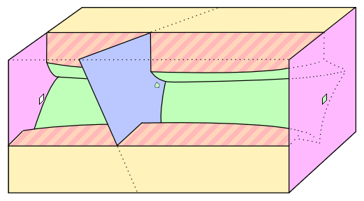
Figure 3: The template cell for our example of an LT satisfying (A1)-(A6).

Moreover, we insert a ‘bulkhead’ in the middle of the cell, that is, we add an infinitesimally thin scatterer given by the intersection of the plane passing through the center of the cell and orthogonal to the vector $(1,1,1)$, and the cell itself. We punch an off-center, small, polygonal hole through the bulkhead, so that it is possible to go from one “chamber” to the other, but no free (i.e., collisionless) trajectories exist between the two gates of the cell. Notice that by choosing the parameter $h$ large enough, we can ensure that the maximum number of consecutive collisions between the flat facets and the bulkhead is 3.

Next, we argue that this setting verifies (A4). We say that a trajectory that hits a scatterer almost tangentially grazes it. So consider a trajectory that grazes a cigar. If this trajectory has a sizable transversal component (compared to the longitudinal one) then its projection on a transversal section is not far from a grazing orbit in a diamond billiard, which implies that the next bounce is not grazing. Let us hence consider grazing trajectories that are almost longitudinal. In this case, within a certain (bounded above) time, the point will hit the bulkhead in such a way that the next collision is necessarily non-grazing and against a cigar, provided $h$ is not too small. On the other hand, since the “transversal angle” at each intersection point of two cigars is bounded below, no more that a bounded number of collisions can be performed in said time. These arguments will be made more quantitative below.

Finally, the full LT is made up of random algebraic perturbations (in the sense of Section 4) of this local configuration. If the perturbations are i.i.d. in each cell, (A1) is obviously verified. If they are sufficiently small, (A6) holds. As for (A5), it is not hard to see (by ergodicity of the inner dynamics in a cell, if one will) that this assumption is verified as well.

Figure 4: The longitudinal projection of a trajectory in the (purely cylindrical) cell, describing a planar trajectory in a diamond billiard. The indicated part of the boundary represents a ‘zone’ (see text).

At the request of an anonymous referee, we give estimates for the universal constants $L$ and $K_{3}$ for this LT. We begin by considering a periodic tube made up of template cells that—contrary to what we have imposed earlier—have no longitudinal curvature. So the dispersing scatterers are truly cylindrical and, if we neglect the bulkheads, describe the same diamond in each transversal section (Fig. 4). Call $\gamma$ the angle at each vertex of the diamond (so $\gamma=\arccos(1/2\rho)$). Fix $h>10$, say, and $g<10^{-1}$.

Denote by $v_{x}$ and $v_{yz}$, respectively, the longitudinal and trasversal components of the velocity $v$ of the material point (thus, $|v_{x}|^{2}+|v_{yz}|^{2}=1$). The longitudinal projection of a piece of trajectory that does not hit a bulkhead is a (planar) trajectory of the diamond billiard. Consider a collision against a cylinder (for the 3D billiard) with outgoing velocity $v$. Denoting by $\theta\in[0,\pi/2)$ the angle of incidence of $v$ w.r.t. the normal at the collision point and by $\varphi$ the corresponing angle for the projected trajectory, we have $\cos\theta=|v_{yz}|\cos\varphi$.

Let us make a couple of observations on the dynamics in the diamond billiard. To start with, we subdivide its boundary in 4 ‘zones’, each zone being defined as the set of all the boundary points that are closer to a given vertex than to any other (see Fig. 4). Let $M:=\lceil\pi/\gamma\rceil$, i.e., $M$ is the minimum integer $\geq\pi/\gamma$. It can be seen that any trajectory in the diamond can have at most $M$ consecutive collisions in the same zone, and at least one of them will have an angle of incidence $\varphi<(\pi-\gamma)/2$ (to see this, just “linearize” the corners). Also, the time between the first collision in a zone and the first collision in another is bounded below by $L_{1}:=1/\sqrt{2}-\rho$ (this is the semilength of the biggest square inscribed in the diamond).

Coming to three-dimensional trajectories, we distinguish two cases: the trajectories with a good transversal component, defined by $|v_{xy}|\geq 10^{-2}$, and the other ones, which we call almost longitudinal. Starting with either case, we want to find an upper bound for the time before the next “head-on” collision—the parameter $\eta$ that defines “head-on”, cf. (A4), will de determined later. By time-reversibility, twice this upper bound will be a good estimate for $L$.

If a trajectory keeps a good transversal component during its entire visit in a single zone, we know from above that there will be a collision with angle of incidence $\theta\leq\arccos(10^{-2}\sin(\gamma/2))=:\pi/2-\eta$, in a time less than $L_{2}:=2hM$ ($2h$ is an estimate for the horizon of our billiard). If not, we eventually fall in the next case, which we consider right away. An almost longitudinal trajectory will remain such until it hits a bulkhead, and this occurs necessarily within a time $L_{3}:=3h(1-10^{-4})^{-1/2}$. The next collision after that, given the inclination of the bulkhead and that $h>10$, is against a cylinder, with $\theta<\pi/2-\eta$.

So, $L$ can chosen to be $2(L_{2}+L_{3})$. During this time, the point can visit at most $\lceil L/L_{1}\rceil$ zones, therefore an upper bound for the number of collisions it can have is $K_{3}:=\lceil L/L_{1}\rceil M+\lceil 3L/h\rceil$ (the first term estimates the collisions against the cylinders and the second term the collisions against the flat boundaries).

We treat the original LT as a perturbation of the one just considered. If the radius of curvature of the cigars in the longitudinal direction is, say, larger than $100h$, multiplying the above estimates by 100 will certainly work.

References

- [AACG] D. Alonso, R. Artuso, G. Casati and I. Guarneri, Heat conductivity and dynamical instability, Phys. Rev. Lett. 82 (1999), no. 9, 1859–1862.
- [AA] V. I. Arnold and A. Avez, Ergodic problems of classical mechanics, Math. Physics Monograph Series, Benjamin, New York, 1968.
- [At] G. Atkinson, Recurrence for co-cycles and random walks, J. London. Math. Soc. (2) 13 (1976), 486–488.
- [BBT] P. Bachurin, P. Bálint and I. P. Tóth, Local ergodicity for systems with growth properties including multi-dimensional dispersing billiards, Israel J. Math. 167 (2008), 155–175.
- [BCST] P. Bálint, N. Chernov, D. Szász and I. P. Tóth, Multi-dimensional semi-dispersing billiards: singularities and the fundamental theorem, Ann. Henri Poincaré 3 (2002), no. 3, 451–482.
- [B] L. A. Bunimovich, Hyperbolicity and astigmatism, J. Statist. Phys. 101 (2000), no. 1-2, 373–384.
- [BD] L. A. Bunimovich and G. Del Magno, Semi-focusing billiards: hyperbolicity, Comm. Math. Phys. 262 (2006), no. 1, 17–32.
- [CM] N. Chernov and R. Markarian, Introduction to the ergodic theory of chaotic billiards, 2nd ed. Publicações Matemáticas do IMPA., Rio de Janeiro, 2003.
- [CLS] G. Cristadoro, M. Lenci and M. Seri, Recurrence for quenched random Lorentz tubes, Chaos 20 (2010), 023115 (errata corrige in Chaos 20 (2010), 049903).
- [H&al] J. K. Holt et al., Fast mass transport through sub-2-nanometer carbon nanotubes, Science 312 (2006), no. 5776, 1034–1037.
- [KS] A. Katok and J.-M. Strelcyn (in collaboration with F. Ledrappier and F. Przytycki), Invariant manifolds, entropy and billiards; smooth maps with singularities, Lectures Notes in Mahematics 1222, Springer-Verlag, Berlin-New York, 1986.
- [KF] J. C. Kimball and H. L. Frisch, Channeling and the periodic Lorentz gas, Phys. Lett. A 128 (1988), no. 5, 273–276.
- [KSS] A. Krámli, N. Simányi and D. Szász, A “transversal” fundamental theorem for semidispersing billiards, Comm. Math. Phys. 129 (1990), no. 3, 535–560.
- [L1] M. Lenci, Aperiodic Lorentz gas: recurrence and ergodicity, Ergodic Theory Dynam. Systems 23 (2003), no. 3, 869–883.
- [L2] M. Lenci, Typicality of recurrence for Lorentz gases, Ergodic Theory Dynam. Systems 26 (2006), no. 3, 799–820.
- [L3] M. Lenci, Central Limit Theorem and recurrence for random walks in bistochastic random environments, J. Math. Phys. 49 (2008), 125213.
- [LWWZ] B. Li, J. Wang, L. Wang and G. Zhang, Anomalous heat conduction and anomalous diffusion in nonlinear lattices, single walled nanotubes, and billiard gas channels, Chaos 15 (2005), 015121.
- [LW] C. Liverani and M. Wojtkowski, Ergodicity in Hamiltonian systems, in: Dynamics Reported: Expositions in Dynamical Systems (N.S.), 4, Springer-Verlag, Berlin, 1995.
- [Lo] H. A. Lorentz, The motion of electrons in metallic bodies I, II, and III, Koninklijke Akademie van Wetenschappen te Amsterdam, Section of Sciences, 7 (1905), 438–453, 585–593, 684–691.
- [P] Ya. B. Pesin, Characteristic Lyapunov exponents and smooth ergodic theory, Russ. Math. Surveys 32 (1977), no. 4, 55–114.
- [S] K. Schmidt, On joint recurrence, C. R. Acad. Sci. Paris Sér. I Math. 327 (1998), no. 9, 837–842.
- [W] M. Wojtkowski, Design of hyperbolic billiards, Comm. Math. Phys. 273 (2007), no. 2, 283–304.