The Emission Line Properties of Gravitationally-lensed 1.5$<z<$5 Galaxies

Abstract

We present and analyse near-infrared spectroscopy for a sample of 28 gravitationally-lensed star-forming galaxies in the redshift range $1.5<z<5$, observed mostly with the Keck II telescope. With typical magnifications of $\simeq$1.5-4 magnitudes, our survey provides a valuable census of star formation rates, gas-phase metallicities and dynamical masses for a representative sample of low luminosity galaxies seen at a formative period in cosmic history. We find less evolution in the mass-metallicity relation compared to earlier work that focused on more luminous systems with $z\sim 2-3$, especially in the low mass ($\sim 10^{9}$ M_⊙) where our sample is $\sim 0.25$ dex more metal-rich. We interpret this offset as a result of the lower star formation rates (typically a factor of $\sim$10 lower) for a given stellar mass in our sub-luminous systems. Taking this effect into account, we conclude our objects are consistent with a fundamental metallicity relation recently proposed from unlensed observations.

1 Introduction

The period corresponding to the redshift range $2<z<4$ is a formative one in the history of star-forming galaxies. During this era, mass assembly proceeds at its fastest rate and the bulk of the metals that establish present-day trends are likely manufactured. Through comprehensive multi-wavelength surveys, much has been learned about the demographics of galaxies during this period (Shapley et al., 2003; van Dokkum et al., 2003; Chapman et al., 2005) as summarized in recent global measures (Hopkins & Beacom, 2006; Ellis, 2008).

Attention is now focusing on the detailed properties of selected star-forming sources in this redshift range. Integral field unit (IFU) spectrographs aided by adaptive optics correction on ground-based telescopes have delivered resolved velocity fields for various $z>2$ galaxy samples revealing systemic rotation in a significant subset (Genzel et al., 2006, 2008; Förster Schreiber et al., 2006, 2009; Law et al., 2007, 2009; Stark et al., 2008; Jones et al., 2010b). Near-infrared spectroscopy, sampling rest-frame optical nebular emission lines, defines the ongoing star formation rate and the gas-phase metallicity (Erb et al., 2006b; Mannucci et al., 2009). Metallicity has emerged as a key parameter since it measures the fraction of baryonic material already converted into stars. Quantitative measures can thus be used to test feedback processes proposed to regulate star formation during an important period in cosmic history.

A fundamental relation underpinning such studies is the mass-metallicity relation first noted locally by Lequeux et al. (1979) and recently quantified in the SDSS survey by Tremonti et al. (2004). The oft-quoted explanation for the relation invokes star-formation driven outflows, e.g. from energetic supernovae, which have a larger effect in low mass galaxies with weaker gravitational potentials. However, other effects may enter, particularly at high redshifts where star formation timescales and feedback processes and their mass dependence likely differ.

Motivated by the above, much observational effort has been invested to measure evolution in the mass-metallicity relation with redshift. The relationship has been defined using galaxy samples extending beyond $z\simeq 1$ (Lamareille et al., 2009; Pérez-Montero et al., 2009) and $z\simeq 2$ (Erb et al., 2006b; Halliday et al., 2008; Hayashi et al., 2009). Most recently, Mannucci et al. (2009) have studied the properties of 10 Lyman-break galaxies (LBGs) at $z\simeq 3$. These pioneering surveys have demonstrated clear evolution with metallicities that decrease at earlier times for a fixed stellar mass.

Inevitably as one probes to higher redshift, it becomes progressively harder to maintain a useful dynamic range in the stellar mass and galaxy luminosity. In the case of most distant studies (e.g. Mannucci et al. 2009), only with long integrations can the mass-metallicity relation be extended down to masses of $10^{9}\,M_{\odot}$, Samples defined via searches through gravitational lensing clusters are a much more efficient probe of this important low mass regime. LBGs lensed by massive foreground clusters can be magnified by 2-3 magnitudes thereby probing intrinsically less massive systems. Initial results using this technique have been presented for small samples by Lemoine-Busserolle et al. (2003), Hainline et al. (2009) and Bian et al. (2010).

As part of a long-term program to determine the resolved dynamical properties of sub-luminous $z>2$ galaxies, we identified a large sample ($\simeq$30) of gravitationally-lensed systems with $z>$1.5 in the HST archive (Sand et al., 2005; Smith et al., 2005; Richard et al., 2010b) and embarked upon a systematic spectroscopic survey with the Keck II Near Infrared Spectrograph (NIRSPEC) to determine their emission line characteristics. The initial motivation was to use the high efficiency of NIRSPEC to screen each target prior to more detailed follow-up with IFU spectrographs sampling the star formation rate and velocity field across each source (Jones et al. 2010b, Livermore et al. in preparation). However, a further product of this extensive spectroscopic survey is detailed information on the star-formation rate, emission line ratios, and line widths for a large sample of lensed $z>1.5$ galaxies. Our eventual sample comprises 28 objects including 5 from the literature mentioned above. The goal of this paper is thus to utilize this sample to extend studies of the mass-metallicity relation and related issues to more representative lower luminosity galaxies at early times.

The paper is structured as follows. Section 2 introduces our sample and discusses the various NIRSPEC observations and their reductions as well as associated Spitzer data necessary to derive stellar masses. Section 3 discusses the mass-metallicity relation and the relationship between dynamical mass and stellar mass noting that a subset of our sample has more detailed resolved data (Jones et al. 2010b, a). We discuss the implications of our results in the context of measurements made of more luminous systems in Section 4.

Throughout the paper, we assume a $\Lambda$-CDM cosmology with $\Omega_{\Lambda}$=0.7, $\Omega_{m}$=0.3 and $h=0.7$. For this cosmology and at the typical redshift $z\sim 2.5$ of our sources, 1″ on sky corresponds to $\sim$8.2 kpc. All magnitudes are given in the AB system.

2 Observations and Data Reduction

2.1 Lensed Sample

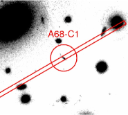
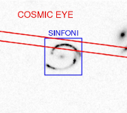
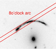
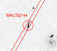
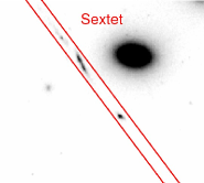
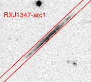
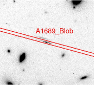
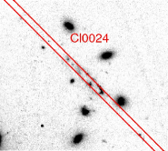
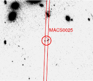
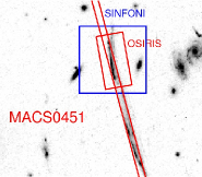
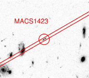
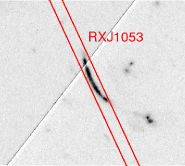
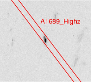
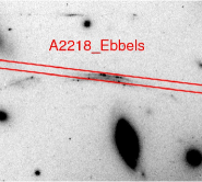
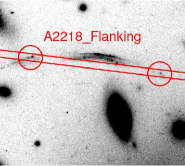
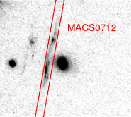
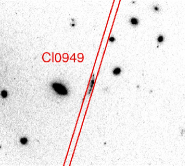
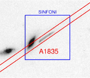
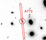
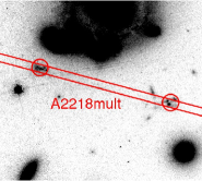
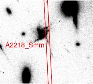
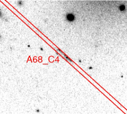
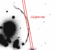
Figure 1: Thumbnail HST images (V band) for each source targeted for near-infrared spectroscopy, showing the orientation of the corresponding NIRSPEC long slit. Targets are marked where there is otherwise ambiguity.

We selected a sample of lensed galaxies for NIRSPEC follow-up using criteria similar to those used for for near-infrared spectroscopy of LBGs (e.g. Erb et al. 2006b) but extended to lower intrinsic luminosities after correction for the lensing magnification. The relevant criteria are:

• Availability of optical data from the Hubble Space Telescope indicating a prominent rest-frame UV continuum with $V<24$

• Spectroscopic redshift $z>1.5$ derived from the literature or as part of our Keck spectroscopic campaign (Richard et al. 2007, 2009, 2010b, Richard et al. 2010c in preparation)

• An areal magnification factor $\mu\mathrel{\hbox{\hbox to0.0pt{\hbox{\lower 4.0pt\hbox{$\sim$}}\hss}\hbox{$>$}}}1.5$ mag provided by the foreground lensing cluster for which a well-constrained mass model enables a good understanding of the associated errors ( e.g. Richard et al. 2010b, Appendix A)

• Emission lines predicted to lie in an uncontaminated region of the near-infrared night sky spectrum

The application of these criteria generated a list of $\sim$ 50 arcs for further follow-up. We summarize in Table 1 the 23 sources drawn from this master list for which we were able to measure significant emission line fluxes. We have augmented this sample with ISAAC archival data and data from the literature for 5 other targets (see Sect. 2.2.2). In total, we consider data for 28 lensed sources spanning the redshift range 1.5$<z<$4.86.

2.2 Near-infrared spectroscopic data

2.2.1 NIRSPEC observations and data reduction

The bulk of the spectroscopic survey was conducted with the NIRSPEC spectrograph (McLean et al. 1998) on the Keck II telescope in its low resolution mode during 7 observing runs (Table 2). A 42 $\times$0.76″long slit was oriented along the major axis of each object, usually the direction of the highest magnification, in order to maximize the line fluxes (Fig. 1). At this resolution, a different wavelength setup was selected for each target (filters N1 to N7, corresponding to the $z^{\prime}$ to $K$ bands) for each group of lines ([Oii], H$\beta$+[Oiii]_{λλ4959,5007}, H$\alpha$+[Nii]+[Sii]).

A major advantage of targeting lensed sources is the ability to survey a large sample of low luminosity sources in an economic amount of observing time. We typically undertook 2 to 4 dithered exposures of 300 - 600 secs each, depending on the magnitude of the source and the sky levels in a given band. We used a three point dithering pattern with offsets larger than the size of the object along the slit. Standard stars were used as flux calibrators. Simultaneously with the NIRSPEC integrations, we took a series of 4-8 short exposures using the slit viewing camera, SCAM, in order to monitor the seeing and slit alignment with the object.

The data was reduced using IDL scripts following the procedure described in more detail in Stark et al. (2007) and Richard et al. (2008). Although the 2D spectrum is distorted on the detector, sky subtraction, wavelength and flux calibration were accomplished in the distorted frame, thereby mitigating any deleterious effect of resampling (see Kelson 2003 for more details).

In comparison with the general procedure applied by Stark et al. (2007) for point sources, we took special care to prevent sky over-subtraction for our bright and extended sources.

2.2.2 Archival, literature and IFU data

A modest amount of additional data on lensed galaxies is available in the literature, in the archive, or through new IFU data. To date, the Keck survey described above represents the major advance.

We included data from the ISAAC instrument on the ESO VLT on 2 lensed galaxies at $z$=1.9 (Lemoine-Busserolle et al., 2003). Additional NIRSPEC data has been published for two suitable objects by Hainline et al. (2009). Finally, we retrieved ISAAC archival data for the giant arc in Cl2244 (Hammer et al., 1989) at $z=2.24$ which was studied by Lemoine-Busserolle et al. (2004). These archival J, H and K-band spectra have been reduced with standard IRAF scripts, following the procedure used in Richard et al. (2003). These 5 additional sources are listed separately in Table 1.

Together with the IFU data presented in Jones et al. (2010b), three of the targets described above (the cosmic eye, A1835 and MACS0451) were observed with the SINFONI integral field spectrograph on the VLT between May 2009 and September 2010 as part of program 083.B-0108. In all three cases we used a 8$\times$8^′′ configuration at a spatial resolution of 0.25^′′/pixel and used $J$, $H$ and $K$-band gratings which result in a spectral resolution of $\lambda$/$\Delta\lambda$=4000 We used ABBA chop sequences while keeping the object inside the IFU at all times. Typical integration times were 7.2 ks (split into 600 second exposures) in $<$0.6^′′ seeing and photometric conditions. Individual exposures were reduced using the SINFONI esorex data reduction pipeline and custom idl routines which, together, extracts, flatfields, wavelength calibrates the data and forms the data cube. The final data cube was generated by aligning the individual data-cubes and then combining the using an average with a 3$\sigma$ clip to reject cosmic rays. For flux calibration, standard stars were observed each night during either immediately before or after the science exposures. These were reduced in an identical manner to the science observations. Detailed analysis of the spatially resolved properties will be discussed in a forthcoming paper (Livermore et al. 2011 in preparation), but here we concentrate on the galaxy integrated emission line properties measured from these observations.

2.2.3 Line fluxes and line widths

Figure 2: Typical extracted NIRSPEC spectra (flux units in erg s^-1 cm^-2 Å^-1) of various signal-to-noise ratios. For RXJ1053, the key nebular lines were covered using 3 different spectrograph settings (shown). Note the detection of [Sii] emission for MACS0744. The dotted line indicates the 1$\sigma$ error on the spectral flux.

Typical reduced spectra are shown in Figure 2. Line fluxes were measured using the IRAF task splot which uses both the science spectrum and the 1$\sigma$ error spectrum obtained from the extraction to derive the total flux and a bootstrap error. The line widths were measured on the highest signal-to-noise ($>10$) spectra, and corrected for the effects of instrumental resolution. Results are given in Table 4. We fit a single Gaussian to the H$\alpha$ and [Oiii]$\lambda 5007$ lines, and a double Gaussian to [Oii] with the lines fixed at rest wavelengths of 3726.1,3728.8 Å. We constrain the [Oii] lines to have the same width and an intensity ratio $I(3726.1)/I(3728.8)\sim 1$ as seen in high redshift galaxies observed with higher spectral resolution (e.g. Swinbank et al. 2009).

The spectral resolution $R=\lambda/FWHM$ measured from bright, unblended OH sky lines in the NIRSPEC spectra is found to vary linearly with spectral order $m$ as expected, and the ratio $R/m$ varies smoothly with wavelength from roughly 2100 at $\lambda=1\,\mu$m ($m=4$) to 4000 at $2.2\,\mu$m ($m=2$). This results in an instrumental FWHM ranging from $160$–260 km/s ($\sigma=70$–110 km/s) for the lines observed in this work. Measured line widths exceed the instrumental resolution in all but one case (RXJ1347-11), for which the 1$\sigma$ upper bound is given in Table 4.

The uncertainty in the line widths is propagated from the 1$\sigma$ error spectrum. Gaussian fits used to determine the line width have residuals $\chi^{2}_{\nu}\simeq 1$ suggesting that the error spectrum is a good estimate of the intrinsic noise. After subtracting the instrumental resolution in quadrature, line widths are typically determined to $\sim$10% accuracy. The uncertainty is significantly larger in cases where the line of interest is blended with a sky line, or has a width close to the instrumental resolution. We estimate any systematic uncertainty in the measured instrumental resolution to be $<3$% based on independent measurements of multiple bright sky lines, hence we expect measurement errors to dominate.

We can test whether the velocity dispersions measured with NIRSPEC are reliable, where there is overlap with integral field data, by undertaking a comparison with the more extensive 2D velocity data (Law et al., 2009; Förster Schreiber et al., 2009; Jones et al., 2010b). Here we enlarge the comparison sample by considering all relevant NIRSPEC data (Erb et al., 2006b). As Fig. 3 shows, the data is in general agreement with the mean IFU velocity dispersion being $1.2\pm 0.3$ times that measured with NIRSPEC. This suggests that the longslit data provide a reasonable estimate of the global galaxy dynamics and cab be used, for example, with the spatial extent to measure dynamical masses.

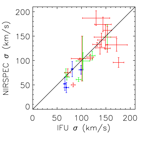
Figure 3: Comparison of the velocity dispersion measured from our long slit NIRSPEC data with 2D integral field unit data from various sources. Blue points refer to mean dispersions ($\sigma$) from OSIRIS IFU observations reported in Jones et al. (2010b). Green crosses show equivalent OSIRIS data from Law et al. (2009) and red crosses are integrated velocity dispersions from the SINFONI IFU (Förster Schreiber et al., 2009). NIRSPEC measurements for the latter samples are reported in Erb et al. (2006b).

2.2.4 Line ratios from stacked spectra

One of our aims is to measure the mass-metallicity relation in our sample, extending it to low-luminosity sources. Given the short exposure times for our survey which has enabled such a large sample to be constructed, inevitably many of the fainter diagnostic lines, e.g. [Nii] and [Sii] are not always visible in individual spectra. In order to estimate the typical prevalence of such faint emission lines, we construct a stacked spectrum about the H$\alpha$ line.

This has been done for two cases. Firstly, for all 9 lensed sources where H$\alpha$ is detected at S/N $>10$, and, secondly, for all 6 cases where the stellar mass (§2.4) is $<3\times 10^{9}$ M_⊙. First we resample the H$\alpha$ spectra into the rest frame with a common dispersion of $1$ Å, and then scale each spectra to a common H$\alpha$ flux. We reject the minimum and maximum values at each wavelength in order to remove outliers (due to sky line residuals, for example), and average the remaining data. The results are consistent with Gaussian noise. The composite spectra are shown in Figure 4.

We measure line ratios in the stacked spectra by fitting a Gaussian profile to H$\alpha$, then using the position and line width to determine the [Nii] and [Sii] fluxes and their bootstrap error. The resulting ratios are provided at the bottom of Table 3.

Figure 4: Stacked spectra chosen to reveal fainter emission lines. Top: stack of all lensed sources with S/N $>10$ in the H$\alpha$ line. Bottom: stack of lensed sources with stellar mass $<3\times 10^{9}$ M_⊙. Dotted lines show the positions of H$\alpha$, [Nii]$\lambda\lambda 6548,6584$, and [Sii]$\lambda\lambda 6717,6731$.

2.2.5 Aperture corrections and further checks

One obvious limitation of long-slit spectroscopy is a significant fraction of the line flux may be missing, especially for the most extended objects or in poor seeing conditions. Our slit width was 0.76 arcsec and so the latter may be a concern for some objects (see Table 2). In order to compare measurements based on long-slit spectroscopy with photometric estimates derived from imaging (see Sect. 2.4), we carefully estimated aperture correction factors.

The procedure adopted was the following: we used the SExtractor segmentation map to select those pixels of the HST image associated with the object. We smoothed this new image by our estimate of the seeing conditions (Table 2) and measured the fraction of the total flux falling inside the region covered by the long slit. We found aperture correction factors between 1.2 and 2.9 depending on the object. The error on these corrections was estimated using a $\pm 0.2$″error on the location of the slit, as checked from the SCAM images. The correction factors are later used to derive the total star formation rate (SFR) of the object, assuming the measured equivalent width of the lines are representative of its average across the entire galaxy. Of course, the metallicity and line ratio measurements are unaffected as they rely entirely on the spectroscopic data. We also checked that measurements of the 8 o’clock arc are consistent with the results presented by Finkelstein et al. (2009).

Six sources in our sample have been presented by Jones et al. (2010b) and were therefore covered both with NIRSPEC and OSIRIS. This allows us to perform a further check on the aperture correction factors. We found that the total line fluxes agree for each object within 10%, which is likely due to the aperture correction and/or the relative flux calibrations. We adopt this 10% error estimate on the total line flux when estimating the SFRs later in the paper.

As mentioned earlier, we can use the same six targets to compare the velocity dispersions estimated from the NIRSPEC and OSIRIS data on the same emission lines (§2.2.3). Although the long slit estimates have larger error bars, they are consistent (within 1$\sigma$) with the more reliable IFU estimates. Nonetheless, we adopt the IFU value whenever availble.

2.3 Magnification and source reconstruction

In order to correct all physical properties (star-formation rates, masses, physical scales) for the lensing magnification, we correct each source for its corresponding magnification factor $\mu$ which stretches the physical scales of each object while keeping its surface brightness fixed. As discussed in §2.1, our targets were specifically chosen to lie in the fields of clusters whose mass models are well-constrained from associated spectroscopy of many lensed sources and multiple-images (see example in Appendix A and Richard et al. (2010b) for further discussion).

The values of $\mu$ are obtained through modeling of the cluster mass distribution using the Lenstool software (see references in Table 1), or from the literature (for the additional targets in Table 1). The relative error on $\mu$, when derived from a Lenstool parametric model, follows a Bayesian MCMC sampler (Jullo et al., 2007) which analyses a family of models fitting the constraints on the multiple images. In Table 1 we report the final values of $\mu$ and their associated errors; these are used to correct $\mu$-dependent physical parameters (star-formation rates and masses) throughout the rest of the paper. Note that the magnification factor does not affect any of the line ratios measurements.

We also construct the demagnified (unlensed) source morphology of each arc modeled with Lenstool by ray-tracing the high-resolution HST image back to the source plane, using the best fit lens model. By comparing the sizes of the observed and reconstructed image of a given target, we can verify the agreement of the magnification factor used and this size ratio (c.f. discussion in Jones et al. 2010b).

2.4 Photometric measurements

A large variety of space- and ground-based images are available for each object from archival sources. All HST images (optical and near-infrared) have been reduced using the multidrizzle package (Koekemoer et al., 2002), as well as specific IRAF scripts for NICMOS data, as described in Richard et al. (2008). Ground-based near-infrared images were reduced following the full reduction procedure described in Richard et al. (2006), and calibrated using 2MASS stars identified in the field.

Archival IRAC data in the first 2 channels (3.6 and 4.5 $\mu$m) are available for all sources except MACS1423, but we only consider sources which are not contaminated by nearby bright galaxies when deriving their photometry. We combine the post-BCD (Basic Calibrated Data) frames resampled to a pixel scale of 0.6″.

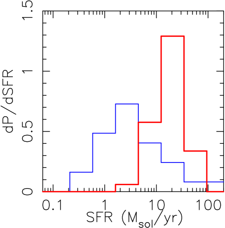
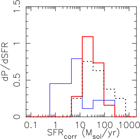
Figure 5: Probability distribution of star-formation rates in our sample of lensed objects (blue histogram) compared to the samples of LBGs at $z\sim 2$ (red histogram, Erb et al. 2006b) and at $z\sim 3$ (dotted histogram, AMAZE and LSD samples,Maiolino et al. 2008 and Mannucci et al. 2009). The left panel compares the distribution of SFR before correcting for extinction, while the right panel compares the values after applying the extinction correction.

The HST image providing the highest signal-to-noise was used to measure the integrated brightness with SExtractor (Bertin & Arnouts, 1996), whereas the double image mode was used to measure the relative HST colours inside a 1″aperture. A small aperture correction is applied to all HST photometry to deal with the PSF differences between the different ACS, WFPC2 and NICMOS bands. In the case of ground-based colours, the primary HST image was smoothed by a Gaussian kernel corresponding to the measured seeing, and convolved with the IRAC PSF (derived from bright unsaturated stars in the image) in order to incorporate IRAC colours. The full photometry is summarised in Table 6 in appendix.

3 Physical Properties of the Sample

Table 4 summarises the derived quantities which will form the basis of our analysis. We now discuss the physical measures in turn.

3.1 Star formation rate and AGN contribution

The intrinsic star formation rate (SFR) is estimated from the total (aperture-corrected) flux in the Balmer lines ($f_{\rm H\alpha}$ and $f_{\rm H\beta}$) based on the well-constrained calibrations by Kennicutt (1998), including the correction for magnification factor $\mu$ and its associated error. In the absence of H$\alpha$ we assume a typical ratio H$\alpha/$H$\beta$=2.86. For two objects (RXJ1347 and A1689-Highz), neither H$\alpha$ nor H$\beta$ is available, therefore we use the [Oii] line to derive the SFR, although it is a less robust estimator because of metallicity and excitation effects (e.g. Gallagher et al. 1989).

The derived values of SFR span a wide range, between 0.4 and 50 M_⊙/yr, and are typically a factor of 10 lower than other samples of LBGs with emission line measurements (Fig. 5). The majority (16 objects) of the lensed sources have SFR$<4$M_⊙/yr, values which are absent from the samples of Erb et al. (2006b) and Maiolino et al. (2008).

An independent estimate of the SFR can be obtained for every object using the ultraviolet continuum luminosity ($L_{\nu}$) estimated at 1500 Å rest-frame. We measure $L_{\nu}$ by fitting a power-law $f_{\lambda}\propto\lambda^{-\beta}$ to the broad-band photometry between 1500 and 4000 Å rest-frame. The UV slope ($\beta$) is given in the first column of Table 6. A value $\beta=2.0$ (constant AB magnitude) is assumed when only a single photometric datapoint was available. The SFR derived from the UV-continuum is then given by Kennicutt (1998).

We can determine from nebular line ratios whether there is a strong contribution from active galaxy nuclei (AGN) in the line emissions. This is done through the diagram of Baldwin et al. (1981) (BPT diagram), where we overplot the location of our targets in Fig. 6.

The majority of our sources lie in the region of the BPT diagram where star-forming galaxies are commonly found (Kewley et al., 2001). MACS0451 and AC114-A2, however, lie close to the boundary with the region occupied by AGNs. We consider it unlikely, however, that these objects are AGN-dominated, because of the lack of X-ray emission in Chandra data and C_IV lines in the optical spectra. Furthermore, the Spitzer data shows evidence for the 1.6$\mu$m rest-frame stellar bump and no sign of obscured AGN activity, which would produce a raising slope in the redder IRAC channels (e.g., Hainline et al. 2010). The location of these objects in the BPT plane simply suggests a higher radiation field, similar to that seen in local starbursts and the sample of LBGs studied by Erb et al. (2006a) at $z\sim 2$ (see also Sect 3.5). We thus conclude that the nebular emission we see in our sources arises from intense star formation.

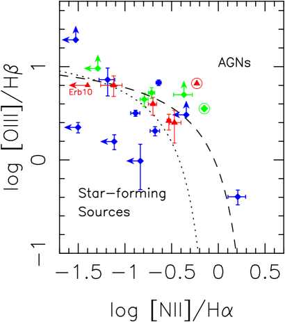
Figure 6: Location of the NIRSPEC targets (blue diamonds) over the BPT diagram, used as a diagnostic for AGN vs star-formation (see text for details). The dotted line is the empirical separation between star-forming and AGN objects from Kauffmann et al. (2003), and the dashed line the theoretical separation from Kewley et al. (2001). Other sources from the literature are shown as green points (lensed objects from Hainline et al. 2009 and lemoine03) or red triangles (Erb et al., 2006b, 2010). The two circled points are objects showing signs of AGN activity, as discussed within these papers.

3.2 Extinction

Dust extinction plays an important role when deriving the physical properties of galaxies, as it will affect the observed line fluxes and some of the line ratios. One of the estimators we can use to measure this extinction is the UV spectral slope $\beta$, which is related to the extinction affecting the young stars. We can also use the ratio between the two SFR estimates (from the observed UV continuum and the H$\alpha$ emission lines) as an independent estimator, as it reflects the differential extinction between the two wavelengths. Note that even in the case of a perfect reddening correction, the nebular emission and the UV do not probe star-formation on the same timescales (Kennicutt, 1998).

Figure 7 compares both estimates for a subsample of the lensed objects, together with the relation predicted by the Calzetti et al. (2000) extinction law. It shows that there is a general agreement with the theoretical predictions, although with quite a large scatter. One of the reasons for the differences is probably a different extinction factor affecting the young and old stellar populations, or a measurement bias towards low extinction regions when measuring $\beta$. This is illustrated by the location of the sub-millimetre lensed galaxy A2218-smm (Kneib et al., 2004), which has a high extinction but a measured slope $\beta=1.6$ (white diamond in Fig. 7).

One way to overcome this issue is to use the full SED (from rest-frame UV to near-infrared) in order to derive the best extinction estimate E(B-V) assuming the Calzetti et al. (2000) law (see Sect.3.3.1). 8 objects in our sample also have both H_α and H_β detected, and the corresponding values of the Balmer decrement range between 2.5 and 4.5, consistent with $0<E(B-V)<0.35$ although with large uncertainties.

We use the best-fit E(B-V) values, given in Table 4, to correct the SFRs, individual line ratios and metallicities in the next sections. In particular, reddening has a strong effect on individual SFRs, and it is very sensitive to unknown factors (differential reddening in a given object, presence of dust in the lightpath through the galaxy cluster, deviation from the Calzetti law as pointed out by Siana et al. 2009). We present both the uncorrected and the extinction-corrected (SFR_corr) in Table 4 and when comparing with other samples (Fig. 5).

Figure 7: Comparison between the SFR estimated from the UV continuum and the H$\alpha$ emission line, as a function of the UV slope $\beta$. The solid curve is the theoretical prediction for the relation between the two values using the Calzetti et al. (2000) extinction law.

3.3 Masses

Two mass estimators can be derived from the available data. Multi-wavelength broad-band photometry gives us access to the stellar mass, through the modelling of the SED, while measuring the widths of the most prominent spectral lines allow us to infer dynamical masses, which should be closer to the total baryonic mass of these galaxies.

3.3.1 Stellar masses

Our stellar masses are derived using the precepts discussed in detail by Stark et al. (2009). We derive the stellar masses for our sample by fitting the Charlot & Bruzual (2007, S. Charlot, private communication) stellar population synthesis models to the observed SEDs. We consider exponentially-decaying star formation histories with the form $\rm{SFR(t)}\simeq exp(-t\tau)$ with e-folding times of $\tau=10$, 70, 100, 300, and 500 Myr in addition to models with continuous star formation (CSF). For a given galaxy, we consider models ranging in age from 10 Myr to the age of the Universe at the galaxy’s redshift. We use a Salpeter (1955) initial mass function (IMF) and the Calzetti et al. (2000) dust extinction law. Finally, we allow the metallicity to vary between solar (Z_⊙) and 0.2 Z_⊙, the range found for the gas-phase metallicity using nebular line ratios (Sect. 3.4). We account for the intergalactic medium absorption following Meiksin (2006). The best fit values of the stellar mass M_∗ and extinction E(B-V) are summarised in Table 4.

We note that the presence of strong emission lines may affect the broad-band photometry and therefore the mass estimates. We estimate the contribution of the strongest emission lines affecting the $H$ and $K$ band magnitudes. In the most extreme cases (largest equivalent widths) the H and K band flux would be affected by at most 5-10%, which does not have a significant effect compared to our estimated errors.

3.3.2 Dynamical masses

We now use the velocity dispersions $\sigma$ (measured in Sect. 2.2.3) to estimate of the dynamical mass. We will express the virial masses M_dyn of our objects as a function of $\sigma$ and their typical size.

Assuming the idealized case of a sphere of uniform density (Pettini et al., 2001) we have:

$M_{dyn}=Cr_{1/2}\sigma^{2}/G$ with $C=5$ or more conveniently,

$$M_{dyn}=1.16\times 10^{10}\ M_{\odot}\frac{\sigma^{2}}{(100\ {\rm km}\ {\rm s}^{-1})^{2}}\frac{r_{1/2}}{\rm kpc}$$ (1)

where $r_{1/2}$ is the half-light radius, which we measure on the source plane reconstructions of our targets (see Sect. 2.3) using the FLUX_RADIUS parameter from SExtractor. This parameter estimates a circularized size corresponding to half of the total detected fluxes. Thanks to the high magnification our sources are well resolved in the HST images, but the main source of error in estimating $r_{1/2}$ (which has a strong impact on M_dyn) is the source reconstruction itself. We produced 100 reconstructions of each source sampling the different parameters of the lens model, using the MCMC sampler described in Sect. 2.3, and use them to derive the mean and dispersion on the measured $r_{1/2}$. We also checked this measurement independently using a half-light radius defined with the Petrosian radius at 20% of the central flux of the object, similar to the work done by Swinbank et al. (2010), and found consistent results.

The values of $r_{1/2}$ and $M_{dyn}$ are reported in Table 4. We note that the geometric correction factor C can vary significantly and is likely between 3 and 10 for these highly turbulent galaxies (Erb et al., 2006b). Hence the true dynamical mass can differ by up to a factor of 2, while uncertainty in the radius and $\sigma$ is much smaller. Our choice of $C=5$ gives slightly higher dynamical masses than in some other studies (e.g. $C=3.4$, Erb et al. 2006b; Bouché et al. 2007).

3.3.3 Comparison

The range of stellar masses spanned by our lensed objects (typically 5 10⁸ - 5 10¹⁰ M_⊙ is lower by a factor of 3-5 than those surveyed by Erb et al. (2006c); Maiolino et al. (2008) and Mannucci et al. (2009) (Fig. 8, left). Within the subsample with reliable dynamical masses, we can directly compare the dynamical and stellar masses. Although we discover a large dispersion (Fig. 8, right), the average ratio $<log(M_{dyn}/M*)>=0.36$ dex is a factor of $\sim 2$, suggesting of $\sim$40% of dynamical mass not present into stars. This value is similar to the result found by Erb et al. (2006c), and confirms the dominance of baryonic mass in the central regions of these galaxies. This was already pointed out by Stark et al. (2008) in the case of the Cosmic Eye. We note that a different choice for the multiplicative factor in Eq. 1 would give $\sim 30$% lower dynamical masses and would strengthen this conclusion.

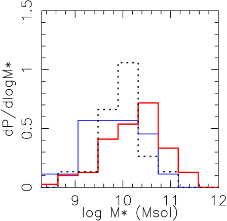
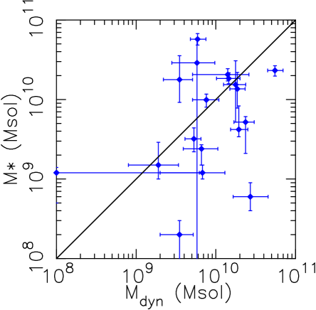
Figure 8: (Left) Probability distribution of stellar masses in our sample of lensed objects (blue histogram) compared to the samples of LBGs at $z\sim 2$ (red histogram, Erb et al. 2006c) and at $z\sim 3$ (dotted histogram, AMAZE and LSD samples, Maiolino et al. 2008 and Mannucci et al. 2009). (Right) Comparison between stellar and dynamical mass estimates. In general we find a higher dynamical mass compared to the stellar mass, suggesting the presence of large amounts of gas mass in this sample.

The gas mass can be evaluated from the SFR and the size of the objects $r_{1/2}$ (ideally assuming the star-formation is uniform over the projected surface seen in the UV), assuming the Kennicutt (1998) law between star-formation rate and gas densities applies at these redshifts. We use this relation to derive the total gas mass:

$$M_{\rm gas}=5.03\ 10^{8}\ {\rm SFR}^{0.71}\ r_{\rm 1/2}^{0.58}\ {\rm M}_{\odot}$$ (2)

Defining the gas fraction $f_{\rm gas}$ as $f_{\rm gas}=M_{\rm gas}/(M_{\rm gas}+M_{*})$ , we find gas fractions ranging from 0.2 to 0.6 after reddening correction, compatible with what is derived from the comparison of stellar and dynamical masses. This is in average $\sim$50% lower that the gas fraction measured by Erb et al. (2006c) at $z\sim 2$ and by Mannucci et al. (2009) in the Lyman-break galaxies Stellar populations and Dynamics (LSD) sample at $z\sim 3$, and reflects the lower SFRs in our objects for a given stellar mass. However, we see the same trend of a lower $f_{\rm gas}$ towards the higher masses.

3.4 Metallicities

The relationship between the oxygen abundance, or gas metallicity $Z$ defined as log(Z)=12+log(O/H), has been accurately calibrated against line ratios of the prominent nebular emission lines (Nagao et al., 2006). Suitable line ratios are available for half of the objects in our sample, and depending on the availability we can combine the estimates from three different metallicity diagnostics, using the recent empirical relations derived by Maiolino et al. (2008) (see also Mannucci et al. 2009).

The prime oxygen abundance indicator is the R23 ratio (Pagel et al., 1979): R23=([Oii]+[Oiii]$\lambda\lambda$4959,5007)/H$\beta$. As the [Oiii]$\lambda$4959 line is usually weakly detected we adopt a canonical value of 0.28 for the [Oiii]$\lambda$4959/[Oiii]$\lambda$5007 ratio. The second estimate for oxygen abundance is the O32 ratio: O32=[Oiii]$\lambda$5007/[Oii]. The final estimate is the N2=[Nii]/H$\alpha$ indicator.

Defining the parameter $x=log(Z/Z_{\odot})$ and using $log(Z_{\odot})$=8.69 (Allende Prieto et al., 2001), we adopt the following fitting formula (Maiolino et al., 2008) on the reddening corrected line ratios:

$\log$(R23)=

$$0.7462-0.7149\ x-0.9401\ x^{2}-0.6154\ x^{3}-0.2524\ x^{4}$$ (3)

$$\log({\rm O32})=-0.2839-1.3881\ x-0.3172\ x^{2}\\$$ (4)

$\log$(N2)=

$$-0.7732+1.2357\ x-0.2811\ x^{2}-0.7201\ x^{3}-0.3330\ x^{4}$$ (5)

These equations provide three different estimates for Z: $Z_{\tt R23}$, $Z_{\tt O32}$ and $Z_{\tt N2}$. Of these, the $Z_{\tt N2}$ and $Z_{\tt R23}$ estimates are the ones showing the lowest dispersion (typically 0.1 dex) while the $Z_{\tt O32}$ estimate has a dispersion of 0.2-0.3 dex. However, the $Z_{\tt R23}$ relation has a “two-branch degeneracy” (e.g. Pettini et al. 2001) between a low-metallicity and a high-metallicity value. In order to discriminate between the two values, we use the $Z_{\tt N2}$ calibration when available (usually synonym of a source on the upper-metallicity branch), otherwise the $Z_{\tt O32}$ calibration. For the 5 sources taken from the literature, we recalculate the best fit Z using the published line fluxes and reddening factors. The resulting value of Z is consistent with the published value except in the case of AC114-S2 Lemoine-Busserolle et al. (2003), where the published value $log(Z)=7.25\pm 0.2$ makes this object a clear outlier in the mass-metallicity relation (Sect. 4.1). Taking the published line fluxes, the N2 limit derived places it at the junction between the two branches of the R23 relation. To resolve this ambiguity we use the values derived with the upper-branch.

The final best-fit value for $\log(Z)$ is reported in Table 4 for each source.The error bars include the typical dispersion in the relation. We find metallicity values ranging from 0.25 Z_⊙ to 1.7 Z_⊙.

3.5 Ionization parameter

In the previous section, the O32 parameter has been used mainly to discriminate between the lower and upper-branch of the R23 calibration of oxygen abundance. For a given metallicity, the O32 line ratio can also be compared with models of Hii regions to measure the ionization parameter $U$, i.e. the ratio of density of ionizing photons over the density of hydrogen atoms (Kewley & Dopita, 2002). Based on early samples of bright LBGs from Pettini et al. (2001), high ionization levels have been measured by Brinchmann et al. (2008), with $\log(U)\sim-2.0$, compared to local samples. This same ionization parameter shifts the objects upward in the BPT diagram (Fig. 6), perhaps pushing the frontier between star-forming galaxies and AGNs (Erb et al., 2006b).

The O32 parameter can be measured for 6 objects in our sample, as well as 2 upper limits, and we obtain values of O32 in the range $0<$O32$<1$. For the range of metallicities found previously (0.2 to 2.0 Z_⊙), we use the curves provided by Kewley & Dopita (2002) to derive ionization parameters $-2.9<\log(U)<-2$ whereas the typical values from local galaxies are in the range $-4<\log(U)<-3$ (Lilly et al., 2003).

This can be illustrated by constructing the O32 vs R23 diagram, as the R23 metallicity estimator has only a weak dependance on the ionization parameter. We overplot the results found by Hainline et al. (2009) on 4 lensed objects (included in our sample) and add our 6 new measurements and 2 upper limits in this diagram (Fig. 9). We can see that , in average, our sample is systematically shifted towards higher values of O32 compared to the lower redshift objects from Lilly et al. (2003). A likely explanation for this effect might be that the physical conditions in the relevant Hii regions are different from those in the local Universe, for example, with larger electron density and/or larger escape fraction (Brinchmann et al., 2008).

An even more extreme result was found recently in a high redshift object by Erb et al. (2010), where they derive an ionization parameter $log(U)\sim 1.0$. The very young age found in this object is one of the factors explaining such a high value of U. Indeed, we can see some trend with age in the O32 vs R23 diagram, despite the small number of objects in our sample. By selecting sources having very young stellar populations (best age $<100$ Myrs from our SED fitting), they all lie in the top part of this diagram, with the highest O32 values.

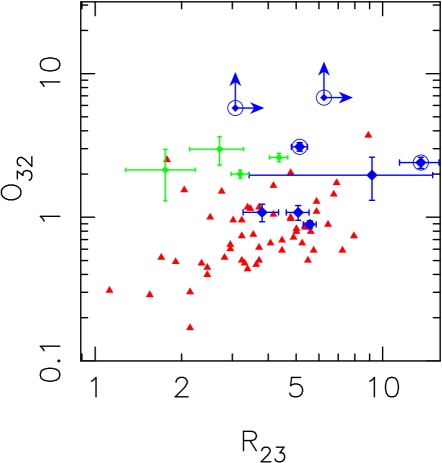
Figure 9: O32 vs R23 diagram, showing the effect of the ionization parameter on O32 (adapted from Hainline et al. 2009). The red triangles are the low redshift ($z<1$) sample of galaxies from Lilly et al. (2003). Our sample of $z>$1.5 lensed galaxies is shown in blue diamonds, while other literature data used by Hainline et al. (2009) is shown in green. Sources in our sample showing young stellar populations (best age $<100$ Myrs from the SED fitting) are circled and typically lie in the top part of the diagram.

4 The Mass Metallicity Relation

4.1 Comparison with Earlier Work

We now compare our measurement of the mass-metallicity relation at high redshift with that of earlier workers recognizing that our data, for the first time, probes to lower masses and lower SFRs by virtue of our selection of gravitationally-lensed systems (Fig. 5 and 8). Figure 10 summarizes the current situation. We find that all galaxies in our sample lie below the well-defined metallicity relation at $z=0.07$ (Tremonti et al., 2004) therefore supporting strongly the case for evolution. Mannucci et al. (2009) have proposed two best fits for this relation, at $z=2.20$ and $z=3.0$, from the Erb et al. (2006a), the AMAZE (Maiolino et al., 2008) and the LSD (Mannucci et al., 2009) samples. If we partition our sample into two redshift bins: $1.5<z<2.5$ and $2.5<z<3.5$, we can see that, on average, the mass-metallicity relation follows these trends. However we observe a large scatter ($\sim 0.25$ dex) in the $1.5<z<2.5$ range and our the evolution implied by our data is less extreme over 2.20$<z<$3.3 than that suggested by Mannucci et al. (2009).

Compared with the earlier unlensed studies, our sample spans a wider range of stellar masses. Therefore, even if our median stellar mass is similar to the $z\sim 3$ sample from Mannucci et al. (2009), we have significantly increased the number of galaxies at $M\sim 10^{9}$ $M_{\odot}$ for the most highly magnified objects. At these masses, we do not seem to see a steep decline in metallicity seen in the $z=2.2$ and $z=3$ best fit found in the earlier surveys (Figure 10). Instead, we see an average shift of $\sim$0.25 dex towards higher metallicities for low-mass objects ($\sim 10^{9}$ M_⊙). Although this trend is limited by the small statistics of our sample, it is also visible when overplotting the results from the composite spectra defined in Sect. 2.2.4.

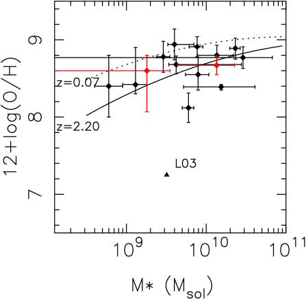
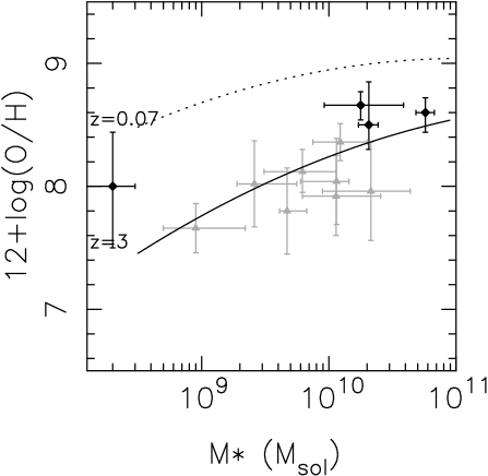
Figure 10: The relation between gas metallicity and stellar mass as a function of redshift. This is based on the diagram presented by Mannucci et al. (2009), with their estimates on $z\sim 3$ galaxies (LSD sample) shown as grey datapoints. The local mass-metallicity relation is showed as a dotted line for $z=0.07$, while their best fit at $z\sim 2.2$ and $z\sim 3.0$ (including both the LSD and AMAZE samples) are shown as solid lines in the left and right panels respectively. We present as diamond symbols the subsample of $1.5<z<2.5$ lensed galaxies in the left panel, and the $2.5<z<3.5$ sample in the right panel. The values derived from the two composite spectra (see Sect. 2.2.4) are shown as red points in the left panel. The original value of $12+log(O/H)$ for AC114-S2 published by Lemoine-Busserolle et al. (2003) is given as a triangle.

4.2 A fundamental metallicity relation?

By comparing the histograms in Fig. 5 and Fig. 8, it is clear that our lensed objects have much lower SFRs than those in more luminous LBGs, even when accounting for the reddening correction, but only slightly smaller masses. Indeed, the effect of the increasing SFR at higher redshift is a usual explanation for the evolution of the mass-metallicity relation seen in Fig. 10, and selecting objects of lower SFR would remove this effect and explain the slight deviation of our sample towards slightly higher metallicity. The reason for the much lower SFR in our sample is expected, as the un-lensed samples of LBGs are selected through their SFR in the UV, while we made no strong assumptions on this parameter.

Recently, Mannucci et al. (2010) have proposed to include the SFR as a third component in the mass-metallicity relation, which would explain its evolution in redshift. One of the reason for the influence of star-formation is that outflows would be more efficient in low-mass objects. Exploring the third-dimensional space defined by stellar mass, gas metallicity and SFR, they fit a surface in low redshift galaxies defined by:

$${\rm Z_{est}}=8.90+0.37\ m-0.14\ s-0.19\ m^{2}+0.12\ m\ s-0.054\ s^{2}$$ (6)

with $m=log(M*)-10$ and $s=log({\rm SFR})$.

By comparing the measured metallicity Z with the projection Z_est estimated from this surface, they managed to reduce the dispersion in SDSS galaxies to $\sim 0.05$ dex. Further computing the distance of higher redshift samples from this surface, they found no significant evolution in this fundamental relation upto $z\sim 2.5$, within the 1$\sigma$ error.

We computed the values of Z_est for each galaxy in our sample and compare it with the measured Z. We find that in average, the best-fit surface predicts the metallicity with no significant offset, and with a scatter of $\sim 0.2$ dex, making this metallicity relation compatible with our measurements within a 2$\sigma$ level. When plotting the distance to the fitted surface as a function of stellar mass (Figure 11) we see no significant trend with stellar mass in both redshift ranges probed by our sample.

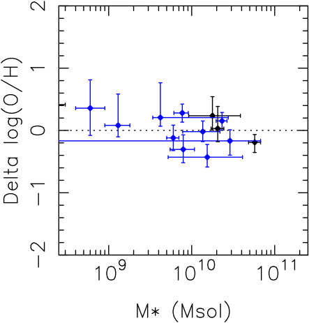
Figure 11: Variation between the measured metallicity and the fundamental metallicity relation proposed by Mannucci et al. (2010), as a function of the stellar mass. Blue/black points are the $1.5<z<2.5$ and $2.5<z<3.5$ subsamples, respectively.The fundamental relation predicts the average metallicity of our lensed galaxies in both redshift ranges.

4.3 Summary and perspectives

We have presented the results of a near-infrared spectroscopy survey targetting 23 bright lensed galaxies at $z>1.5$, complemented by 5 sources from the literature. We summarize here our findings:

• After correction for the magnification factor, our sample shows in average 10$\times$ smaller star-formation rates and 5$\times$ smaller stellar masses than the samples of LBGs at the same redshifts. Such low values of SFR would not be accessible without the strong lensing effect, making our sample complementary to LBG studies.

• The comparison of dynamical and stellar mass estimates reveals the presence of significant gas fractions ($\sim 40$% in average), which are compatible with a simple estimation from their star-formation rate density assuming the Kennicutt (1998) law. We observe typically lower gas fractions in the high mass objects.

• We estimate the ionization parameter $U$ for 8 objects where O32 and R23 line ratios are available, and derive high values with $\log(U)\sim-2.5$. The highest ionization values seem to correlate with the youngest stellar populations ($<100$ Myrs).

• The gas-phase metallicites are calculated combining various line-ratios estimators, and we find a weaker evolution in the mass-metallicity relation compared to estimates from bright LBGs observed in blank fields, with an offset reaching $\sim 0.25$ dex in the low stellar mass range ($\sim 10^{9}$ M_⊙). This effect is seen both in the majority of individual sources as well as in composite spectra created from the highest signal-to-noise or the low-mass objects.

• Assuming that the evolution in the mass-metallicity relation is due to the increasing SFR at higher redshifts, we can reconcile our results with the existence of a fundamental relation of mass, metallicity and SFR as proposed by Mannucci et al. (2010). The weaker evolution in the mass-metallicity relation in our sample is due to lower SFRs (compared to other luminous samples) for only slighly smaller masses.

We foresee that the next HST programs on lensing clusters will continue to detect large number of magnified high redshift galaxies as multiple images, which would be ideal targets for deeper multi-object spectroscopic similar to the current work. This is a unique opportunity to extend the current sample to much lower stellar masses (typically 10⁸ M_⊙) and consequently provide more constraints on the mass-metallicity relation for a wide range of star-formation rates, metallicities and redshifts.

Target	R.A.	Dec.	$z$	Ref. $z$	$\mu$	Ref. $\mu$
	(2000.0)	(2000.0)			(mags)
A68-C1	00:37:06.203	+09:09:17.43	1.583	(1)	2.52$\pm$0.1	(13)
CEYE	21:35:12.712	$-$01:01:43.91	3.074	(2)	3.69$\pm$0.12	(19)
8OCLOCK	00:22:41.009	+14:31:13.81	2.736	(3)	2.72${}^{+0.8}_{-0.4}$	(3)
MACS0744	07:44:47.831	+39:27:25.50	2.209	(4)	3.01$\pm$0.18	(6)
Sextet	13:11:26.466	$-$01:19:56.28	3.042	(5)	4.43$\pm$0.33	(13)
RXJ1347-11	13:47:29.271	$-$11:45:39.47	1.773	(6)	3.61$\pm$0.15	(6)
A1689-Blob	13:11:28.686	$-$01:19:42.54	2.595	(6)	4.70$\pm$1.05	(13)
Cl0024	00:26:34.407	+17:09:54.97	1.679	(7)	1.38$\pm$0.15	(20)
MACS0025	00:25:27.686	$-$12:22:11.23	2.378	(8)	1.75$\pm$0.25	(21)
MACS0451	04:51:57.186	+00:06:14.87	2.013	(4)	4.22$\pm$0.27	(6)
MACS1423	14:23:50.775	+24:04:57.45	2.530	(9)	1.10$\pm$0.12	(9)
RXJ1053	10:53:47.707	+57:35:10.75	2.576	(9b)	4.03$\pm$0.12	Appendix A.
A1689-Highz	13:11:25.445	$-$01:20:51.54	4.860	(10)	1.99$\pm$0.10	(13)
A2218-Ebbels	16:35:49.179	+66:13:06.51	2.518	(11)	3.81$\pm$0.30	(12)
A2218-Flanking	16:35:50.475	+66:13:06.38	2.518	(12)	2.76$\pm$0.21	(12)
MACS0712	07:12:17.534	+59:32:14.96	2.646	(4)	3.60$\pm$0.32	(6)
Cl0949	09:52:49.716	+51:52:43.45	2.394	(13)	2.16$\pm$0.24	(13)
A1835	14:01:00.951	+02:52:23.40	2.071	(13)	4.50$\pm$0.32	(13)
A773	09:17:57.403	+51:43:46.57	2.300	(13)	2.69$\pm$0.35	(13)
A2218-Mult	16:35:48.952	+66:12:13.76	3.104	(12)	3.39$\pm$0.18	(12)
A2218-Smm	16:35:55.033	+66:12:37.01	2.517	(14)	3.01$\pm$0.16	(12)
A68-C4	00:37:07.716	+09:09:06.44	2.622	(1)	4.15$\pm$0.16	(13)
CL2244	22:47:11.728	$-$02:05:40.29	2.240	(15)	4.08$\pm$0.30	(15)
AC114-S2	22:58:48.826	$-$34:47:53.33	1.867	(16)	$2.01\pm 0.17$	(22)
AC114-A2	22:58:47.787	$-$34:48:04.33	1.869	(16)	$1.70\pm 0.15$	(22)
HORSESHOE	11:48:33.140	+19:30:03.20	2.379	(17)	3.70$\pm$0.18	(17)
CLONE	12:06:02.090	+51:42:29.52	2.001	(18)	3.62$\pm$0.12	(24)
J0900+2234	09:00:02.790	+22:34:03.60	2.032	(23)	1.70$\pm$0.08	(23)

(1) Richard et al. (2007) (2) Smail et al. (2007) (3) Allam et al. (2007) (4) Jones et al. (2010b) (5) Frye et al. (2007) (6) Richard et al. 2010c in preparation (7) Broadhurst et al. (2000) (8) Bradač & et al. (2008) (9) Limousin et al. (2010) (9b) Hasinger et al. (1998) (10) Frye et al. (2002) (11) Ebbels et al. (1996) (12) Elíasdóttir et al. (2007) (13) Richard et al. (2010a) (14) Kneib et al. (2004) (15) Mellier et al. (1991) (16) Lemoine-Busserolle et al. (2003) (17) Belokurov et al. (2007) (18) Lin et al. (2009) (19) Dye et al. (2007) (20) Jauzac et al. in preparation (21) Smith et al. (2010) in preparation (22) Campusano et al. (2001) (23) Bian et al. (2010) (24) Jones et al. (2010a)

Table 1: The current sample of lensed galaxies. From left to right: astrometry, redshift and reference, magnification and reference. The sources below the line represent those drawn from the literature.

Run	Date	Seeing (″)	Photometric?
A	2005 October 13	0.5	Photometric
B	2006 July 24	0.8	Clear
C	2007 January 12	1.0	Clear
D	2007 May 3	0.5-0.6	Clear
E	2007 September 1	0.5	Photometric
F	2008 March 23	0.4-0.5	Photometric
G	2008 August 24	0.5-0.9	Clear

Table 2: NIRSPEC observing runs and conditions

ID	$z$	Runs	Filters	[Oii]	H$\beta$	[Oiii]$\lambda 5007$	H$\alpha$	[Nii]	[Sii](a)
A68-C1	1.583	A	N3		$83.6\pm 11.4$	$273\pm 17$
CEYE	3.074	B	N6	$983\pm 92$	$490\pm 22$	$1030\pm 32$
8OCLOCK	2.736	C	N4,N7	$2690\pm 66$			$7450\pm 90$	$1140\pm 37$
MACS0744	2.209	C	N7				$1540\pm 40$	$461\pm 23$	$557\pm 30$
Sextet	3.042	D	N5,N7	$<32$	$200\pm 20$	$850\pm 29.6$
RXJ1347-11	1.773	D	N1	$1130\pm 32$
A1689-Blob	2.595	D	N7				$426\pm 123$	$<39$
Cl0024	1.679	E	N5				$1140\pm 34$	$323\pm 19$
MACS0025	2.378	E	N7				$87\pm 10$	$<66.7$
MACS0451	2.013	E	N6		$1174\pm 61$	$7899\pm 118.$	$3170\pm 59$	$729\pm 30$	$999\pm 45$
MACS1423	2.530	F	N6,N7		$123\pm 40$	$120\pm 22$	$313\pm 39$	$<45.8$
RXJ1053	2.576	F	N3,N6,N7	$510\pm 26$	$624\pm 32$	$1980\pm 44.5$	$1640\pm 42$	$213\pm 18$
A1689-Highz	4.860	F	N7	$43\pm 17$
A2218-Ebbels	2.518	F	N3,N6,N7	$164\pm 13$	$108\pm 11$	$170\pm 13$	$273\pm 18$	$<21$
A2218-Flanking	2.518	F	N6,N7		$180\pm 14$	$402\pm 20$	$444\pm 22$	$<14$
MACS0712	2.646	F	N3,N6,N7	$<32$	$352\pm 20$	$719\pm 40$	$1070\pm 34$	$225\pm 19$
Cl0949	2.394	F	N3,N5,N7	$321\pm 20$	$<42.3$	$819\pm 30$	$403\pm 20$	$<12$
A1835	2.071	F	N5		$400\pm 20$	$879\pm 46$	$1700\pm 150$	$111\pm 20$
A773	2.300	F	N6,N7		$268\pm 21$	$108\pm 11$	$78\pm 9$	$126\pm 12$
A2218-Mult	3.104	G	N4,N6	$1310\pm 40$	$871\pm 31$	$1920\pm 70$
A2218-Smm	2.517	G	N6		$688\pm 29$	$1030\pm 34$
A68-C4	2.622	G	N6		$97\pm 15$	$<22$
CL2244	2.239	ISAAC	J,H,K	$370\pm 80$	$<42$	$67\pm 10$	$463\pm 70$	$<20$
(a) Sum of the [Sii] $\lambda$6717 and $\lambda$6731 line fluxes.
S/N Composite			[Nii]$\lambda 6584$/H$\alpha$=0.16$\pm$0.03, [Sii]$\lambda\lambda 6717,6731$/H$\alpha$=0.11$\pm$0.04
Low M∗ Composite			[Nii]$\lambda 6584$/H$\alpha$=0.13$\pm$0.10

Table 3: Emission line measurements. Fluxes are given in units of 10^-19 ergs s^-1 cm^-2.

ID	$z$	$r_{1/2}$	$\sigma$	Mdyn	M∗	SFR	SFRcorr	log(Z)	E(B-V)
		(kpc)	(km/s)	($10^{10}$ M⊙)	($10^{10}$ M⊙)	(M${}_{\odot}\ yr^{-1})$	(M${}_{\odot}\ yr^{-1})$
A68-C1	1.583	1.09$\pm$0.18	$72^{+16}_{-18}$	$0.66^{+0.40}_{-0.27}$	$0.24_{-0.09}^{+0.03}$	0.8$\pm$0.1	0.9$\pm$0.2		0.02
CEYE	3.074	1.75$\pm$0.21	54$\pm$4(a)	$0.59^{+0.16}_{-0.11}$	$5.74_{-0.90}^{+1.01}$	37.6$\pm$4.3	77.3$\pm$8.8	$8.64^{+0.12}_{-0.16}$	0.17
8OCLOCK	2.736	1.47$\pm$0.38	45$\pm$5	$0.35^{+0.16}_{-0.13}$	$1.78_{-0.86}^{+2.11}$	98.0$\pm$28.	232.$\pm$48.	$8.66^{+0.11}_{-0.12}$	0.22
MACS0744	2.209	1.00$\pm$0.22	$81^{+9}_{-9}$	$0.76^{+0.33}_{-0.25}$	$0.99_{-0.19}^{+0.18}$	6.6$\pm$1.0	11.9$\pm$1.8	$8.91^{+0.13}_{-0.13}$	0.19
Sextet	3.042	0.30$\pm$0.10	$101^{+8}_{-8}$	$0.35^{+0.17}_{-0.15}$	$0.02_{-0.01}^{+0.01}$	1.1$\pm$0.3	2.4$\pm$0.7	$8.00^{+0.44}_{-0.50}$	0.18
RXJ1347-11	1.773	2.48$\pm$0.27	$<46$	$<0.61$	$0.12_{-0.07}^{+0.02}$	2.2$\pm$0.3	5.3$\pm$0.7		0.16
A1689-Blob	2.595				$0.01_{-0.01}^{+0.01}$	0.6$\pm$0.4			0.0
Cl0024	1.679	10.0$\pm$1.2	69$\pm$5(a)	$5.52^{+1.45}_{-1.06}$	$2.32_{-0.35}^{+0.34}$	14.6$\pm$1.9	34.5$\pm$4.6	$8.89^{+0.13}_{-0.14}$	0.28
MACS0025	2.378				$0.16_{-0.09}^{+0.05}$	1.7$\pm$0.4	2.1$\pm$0.5		0.08
MACS0451	2.013	2.50$\pm$0.33	80$\pm$5(a)	$1.86^{+0.47}_{-0.36}$	$1.36_{-0.58}^{+0.83}$	3.4$\pm$0.8	5.9$\pm$1.3	$8.80^{+0.13}_{-0.12}$	0.18
MACS1423	2.530					8.5$\pm$1.4
RXJ1053	2.576	3.62$\pm$0.45	68${}^{+6}_{-6}$	$1.94^{+0.58}_{-0.41}$	$0.42_{-0.08}^{+2.34}$	3.8$\pm$0.4	90.5$\pm$2.3	$8.68^{+0.11}_{-0.12}$	0.37
A1689-Highz	4.860				$0.92_{-0.20}^{+0.24}$	4.2$\pm$1.7			0.0
A2218-Ebbels	2.518				$0.79_{-0.24}^{+0.29}$	0.7$\pm$0.2	1.1$\pm$0.3	$8.37^{+0.20}_{-0.20}$	0.16
A2218-Flanking	2.518	2.36$\pm$0.55	$50^{+17}_{-24}$	$0.68^{+0.62}_{-0.48}$	$0.12_{-0.02}^{+0.03}$	2.3$\pm$0.4	5.5$\pm$1.0		0.28
MACS0712	2.646	0.75$\pm$0.23	$82^{+15}_{-17}$	$0.58^{+0.39}_{-0.30}$	$2.89_{-2.88}^{+3.87}$	3.0$\pm$0.7	5.6$\pm$1.4	$8.77^{+0.14}_{-0.14}$	0.20
Cl0949	2.394	3.50$\pm$0.88	66$\pm 3^{(a)}$	$1.77^{+0.60}_{-0.52}$	$1.54_{-1.02}^{+2.55}$	3.6$\pm$0.7	7.5$\pm$1.5	$8.10^{+0.06}_{-0.05}$	0.24
A1835	2.071	1.52$\pm$0.07	$124^{+39}_{-43}$	$2.71^{+1.82}_{-1.06}$	$0.06_{-0.02}^{+0.03}$	1.1$\pm$0.3	2.5$\pm$0.6	$8.40^{+0.40}_{-0.40}$	0.26
A773	2.300	0.38$\pm$0.05	$66^{+21}_{-29}$	$0.19^{+0.15}_{-0.11}$	$0.15_{-0.05}^{+0.48}$	0.4$\pm$0.1	0.9$\pm$0.3		0.27
A2218-Mult	3.104	3.75$\pm$0.44	$57^{+21}_{-30}$	$1.41^{+1.19}_{-0.90}$	$2.06_{-0.35}^{+0.38}$	18.6$\pm$2.9	216$\pm$34	$8.50^{+0.34}_{-0.23}$	0.58
A2218-Smm	2.517	1.86$\pm$0.40	$82^{+7}_{-7}$	$1.45^{+0.56}_{-0.43}$	$1.84_{-0.26}^{+0.33}$	10.1$\pm$1.4	21.7$\pm$3.1		0.18
A68-C4	2.622				$0.01_{-0.01}^{+0.01}$	0.5$\pm$0.1	0.7$\pm$0.2		0.05
CL2244	2.2399				$0.13_{-0.04}^{+0.05}$	1.4$\pm$0.4	2.1$\pm$0.6	$8.42^{+0.48}_{-0.13}$	0.13
Composite 1	$2.37\pm 0.34$				$0.97_{+3.37}^{-0.75}$			$8.67^{+0.12}_{-0.12}$
Composite 2	$2.52\pm 0.10$				$0.18_{+0.10}^{-0.10}$			$8.64^{+0.19}_{-0.38}$
AC114-S2(b)	1.867			0.53$\pm$0.12	$0.32_{-0.12}^{+0.10}$	30.		8.78$\pm$0.20(e)	0.30
AC114-A2(b)	1.869			2.36$\pm$0.67	$0.52_{-0.09}^{+0.31}$	15.		8.94$\pm$0.20	0.40
HORSESHOE(c)	2.38	2.5		$1.0$		$73.$		8.49$\pm$0.16	0.15
CLONE(c)	2.00	2.9		$2.2$		$32.$		8.51$\pm$0.20	0.24
J0900+2234(d)	2.032			7.2	0.6	116$\pm$16		8.12$\pm$0.19	0.25

^(a)Jones et al. (2010b) ^(b)Lemoine-Busserolle et al. (2003) ^(c)Hainline et al. (2009) ^(d)Bian et al. (2010)

^(e)log(Z) value derived using the upper branch of the R23 diagram (see text for details).

Table 4: Physical properties of the sample. From left to right: ID, redshift, magnification, half-light radius, measured velocity dispersion (corrected from instrumental resolution, see text for details), dynamical mass, stellar mass, SFR, metallicity, stellar extinction from the SED fitting. The SFR and stellar masses are corrected for the lensing magnification factor, and include the aperture corrections. Average redshift and stellar mass are given for the composite spectra described in the text.

Appendix A RXJ1053 mass model

In order to derive the magnification factor for the source at $z=2.576$ in the lensing cluster RXJ1053, we constructed a parametric mass model of the central region of the cluster using the Lenstool software (Jullo et al., 2007). Following similar strong-lensing works (e.g. Richard et al. 2009), we assume the cluster mass distribution to follow a double Pseudo-Isothermal Elliptical (dPIE, Elíasdóttir et al. 2007) profile, and we add two central cluster members as lower-scale perturbations in the mass distribution. This model is constrained by the location of 3 images of the giant arc, clearly detected thanks to their morphology and symmetry on the V-band HST image (Fig. 12). A fourth central image (A4) is predicted by the best fit model and identified on the same image. The best fit model has an rms $\sigma=0.15$” between the predicted and observed positions of the 4 images. We report the best-fit parameters of the mass distribution in Table 5.

Component	$x$	$y$	$e$	$\theta$	$\sigma$	rcore	rcut
	(”)	(”)		(deg.)	(km s-1)	(kpc)	(kpc)
Cluster	$[0]$	$[0]$	0.55$\pm$0.11	52.6$\pm$4.5	705${}^{+169}_{-149}$	60$\pm$23	1000.0
BCG	$[0]$	$[0]$	[0.146]	[41.4]	705$\pm$150	[0.]	39${}^{+40}_{-5}$
Gal1	[2.1]	[4.2]	[0.16]	[42.4]	202$\pm$87	[0.]	20${}^{+30}_{-3}$

Table 5: Best fit parameters for the mass distribution reproducing the multiple components of the giant arc in RXJ1053. The dPIE parameters are given for each component: centre, ellipticity and orientation, velocity dispersion, core and cut radii.

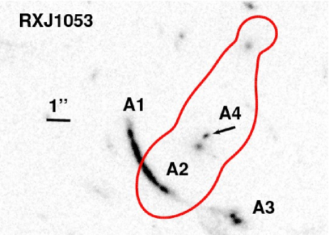
Figure 12: Central region around the BCG of the lensing cluster RXJ1053, showing the giant arc A visible as 4 images A1 to A4. The red line outlines the critical curve at the redshift $z=2.576$ of the source A.

Table 6: Multi-walength photometry (AB magnitudes) of the lensed sources in our sample. First column gives the UV $\beta$ slope (see text for details). We use the notation BB’GVRII’JH as a shortcut for the various HST broad-band filters. Filter names in italics refer to ground-based images.

ID	$\beta$	F450W(B)	F555W(G)	F775W(I’)	F850LP	F110W/$J$	F160W/$H$	$K$/Ks	IRAC 3.6$\mu$m	IRAC 4.5$\mu$m
		F475W(B’)	F606W(V)	F814W(I)
			F702W(R)
8OCLOCK	1.60$\pm$0.15	B 21.94$\pm$0.10	V 21.36$\pm$0.10	I 21.10$\pm$0.10		J 21.12$\pm$0.10	H 20.77$\pm$0.10		20.16$\pm$0.12	19.84$\pm$0.12
A68-C1	[2.0]		R 24.02$\pm$0.04			$J$ 22.41$\pm$0.08	$H$ 22.30$\pm$0.08	$K$ 21.77$\pm$0.22	21.98$\pm$0.15	22.18$\pm$0.15
COSMICEYE	0.38$\pm$0.11		V 20.54$\pm$0.02	I 20.01$\pm$0.05		J 20.07$\pm$0.05	H 19.32$\pm$0.05	$K$ 18.82$\pm$0.10	18.26$\pm$0.15	18.31$\pm$0.15
MACS0744	1.30$\pm$0.07		G 23.04$\pm$0.03	I 22.73$\pm$0.03				Ks 21.22$\pm$0.24	20.45$\pm$0.08	20.42$\pm$0.16
A1689-Sextet	1.77$\pm$0.19	B’ 23.25$\pm$0.05	V 22.36$\pm$0.05	I’ 22.29$\pm$0.05	22.34$\pm$0.05	J 22.36$\pm$0.05	$H$ 21.94$\pm$0.05	$K$ 21.89$\pm$0.05	21.87$\pm$0.05	22.02$\pm$0.05
RXJ1347	1.65$\pm$0.10	B’ 21.61$\pm$0.06		I 21.41$\pm$0.06		$J$ 21.16$\pm$0.18	$H$ 20.52$\pm$0.29	$K$ 20.56$\pm$0.25	20.30$\pm$0.17	20.40$\pm$0.11
A1689-Blob	2.83$\pm$0.15	B’ 23.13$\pm$0.05	V 23.14$\pm$0.05	I’ 23.25$\pm$0.05	23.45$\pm$0.05	J 23.65$\pm$0.05	$H$ 23.28$\pm$0.05	$K$ 23.44$\pm$0.05	22.50$\pm$0.05	22.67$\pm$0.05
Cl0024	1.04$\pm$0.21	B’ 21.78$\pm$0.06	V 21.53$\pm$0.06	I’ 21.32$\pm$0.06	21.10$\pm$0.07	J 20.59$\pm$0.08	H 20.27$\pm$0.08	$K$ 20.12$\pm$0.12	19.56$\pm$0.10	19.58$\pm$0.10
MACS0025	1.77$\pm$0.15		G 23.70$\pm$0.05	I 23.60$\pm$0.08					22.94$\pm$0.17	22.69$\pm$0.13
MACS0451	1.61$\pm$0.21		V 19.60$\pm$0.07	I 19.47$\pm$0.07					17.77$\pm$0.16	17.80$\pm$0.16
MACS1423	2.43$\pm$0.05		V 23.78$\pm$0.06	I 23.70$\pm$0.06				Ks $>23.08$
RXJ1053	[2.0]		V 21.25$\pm$0.05				H 20.01$\pm$0.10
A1689-Highz	3.32$\pm$0.23		V 24.93$\pm$0.05	I’ 23.23$\pm$0.05	23.20$\pm$0.05	J 23.31$\pm$0.05	$H$ 23.66$\pm$0.12	$K$ 22.99$\pm$0.08	22.81$\pm$0.12
A2218-Ebbels	1.89$\pm$0.15	B’ 21.24$\pm$0.11	V 20.75$\pm$0.06	I’ 20.66$\pm$0.06	20.71$\pm$0.06	J 20.44$\pm$0.08	H 19.78 $\pm$0.08	$K$ 19.79$\pm$0.12	19.41$\pm$0.16	19.39$\pm$0.16
A2218-Flanking	1.86$\pm$0.13	B’ 23.32$\pm$0.05	V 22.70$\pm$0.05	I’ 22.61$\pm$0.05	22.65$\pm$0.05	J 22.31$\pm$0.08	H 22.08$\pm$0.09	$K$ 22.17$\pm$0.14
MACS0712	$1.17\pm 0.15$		V 21.93$\pm$0.05	I 21.65$\pm$0.05
Cl0949	[2.0]		V 22.09$\pm$0.05						20.13$\pm$0.20
A1835	$1.76\pm 0.15$		R 21.35$\pm$0.07		21.28$\pm$0.05	$J$ 20.84$\pm$0.07	H 20.87$\pm$0.04	$K$ 20.51$\pm$0.08
A773	[2.0]		R 22.67$\pm$0.05						21.26$\pm$0.12	21.10$\pm$0.14
A2218-Mult	1.22$\pm$0.14	B’ 24.95$\pm$0.16	V 22.23$\pm$0.06	I’ 21.95$\pm$0.05	21.93$\pm$0.05			$K$ 19.91$\pm$0.13	18.93$\pm$0.14	18.74$\pm$0.13
A2218-Smm	1.52$\pm$0.11	B’ 23.52$\pm$0.05	V 23.12$\pm$0.05	I’ 23.13$\pm$0.05	22.97$\pm$0.04	J 22.65 $\pm$0.07	H 21.88$\pm$0.11	$K$ 21.29$\pm$0.14	20.45$\pm$0.12	20.09$\pm$0.13
A68-C4	[2.0]		R 23.31$\pm$0.04			$J$ 22.91$\pm$0.29	$H$ 22.98$\pm$0.35		23.02$\pm$0.12	23.21$\pm$0.15
CL2244	1.76$\pm$0.15		G 21.35$\pm$0.06	I 21.25$\pm$0.06		$J$ 20.74$\pm$0.18	$H$ 20.49$\pm$0.18		20.53$\pm$0.12	20.34$\pm$0.12
AC114-A2	0.98$\pm$0.17		R 22.16$\pm$0.06		21.86$\pm$0.05	$J$ 21.19$\pm$0.18	$H$ 21.30$\pm$0.11	$K$ 20.92$\pm$0.13
AC114-S2	1.25$\pm$0.17		R 22.96$\pm$0.06		22.74$\pm$0.04	$J$ 22.33$\pm$0.07	$H$ 22.21$\pm$0.06	$K$ 22.04$\pm$0.07	21.63$\pm$0.12	21.51$\pm$0.08

References

- Allam et al. (2007) Allam S. S., Tucker D. L., Lin H., Diehl H. T., Annis J., Buckley-Geer E. J., Frieman J. A., 2007, ApJ, 662, L51
- Allende Prieto et al. (2001) Allende Prieto C., Lambert D. L., Asplund M., 2001, ApJ, 556, L63
- Baldwin et al. (1981) Baldwin J. A., Phillips M. M., Terlevich R., 1981, PASP, 93, 5
- Belokurov et al. (2007) Belokurov V., Evans N. W., Moiseev A., King L. J., Hewett P. C., Pettini M., Wyrzykowski L., McMahon R. G., Smith M. C., Gilmore G., Sanchez S. F., Udalski A., Koposov S., Zucker D. B., Walcher C. J., 2007, ApJ, 671, L9
- Bertin & Arnouts (1996) Bertin E., Arnouts S., 1996, A&AS, 117, 393
- Bian et al. (2010) Bian F., Fan X., Bechtold J., McGreer I. D., Just D. W., Sand D. J., Green R. F., Thompson D., Peng C. Y., Seifert W., Ageorges N., Juette M., Knierim V., Buschkamp P., 2010, ApJ, 725, 1877
- Bouché et al. (2007) Bouché N., Cresci G., Davies R., Eisenhauer F., Förster Schreiber N. M., Genzel R., Gillessen S., Lehnert M., Lutz D., Nesvadba N., Shapiro K. L., Sternberg A., Tacconi L. J., Verma A., Cimatti A., Daddi E., Renzini A., Erb D. K., Shapley A., Steidel C. C., 2007, ApJ, 671, 303
- Bradač & et al. (2008) Bradač M., et al., 2008, ApJ, 687, 959
- Brinchmann et al. (2008) Brinchmann J., Pettini M., Charlot S., 2008, MNRAS, 385, 769
- Broadhurst et al. (2000) Broadhurst T., Huang X., Frye B., Ellis R., 2000, ApJ, 534, L15
- Calzetti et al. (2000) Calzetti D., Armus L., Bohlin R. C., Kinney A. L., Koornneef J., Storchi-Bergmann T., 2000, ApJ, 533, 682
- Campusano et al. (2001) Campusano L. E., Pelló R., Kneib J., Le Borgne J., Fort B., Ellis R., Mellier Y., Smail I., 2001, A&A, 378, 394
- Chapman et al. (2005) Chapman S. C., Blain A. W., Smail I., Ivison R. J., 2005, ApJ, 622, 772
- Dye et al. (2007) Dye S., Smail I., Swinbank A. M., Ebeling H., Edge A. C., 2007, MNRAS, 379, 308
- Ebbels et al. (1996) Ebbels T. M. D., Le Borgne J., Pello R., Ellis R. S., Kneib J., Smail I., Sanahuja B., 1996, MNRAS, 281, L75
- Elíasdóttir et al. (2007) Elíasdóttir Á., Limousin M., Richard J., Hjorth J., Kneib J.-P., Natarajan P., Pedersen K., Jullo E., Paraficz D., 2007, ApJ submitted, astro-ph/0710.5636
- Ellis (2008) Ellis R. S., 2008, in Loeb, A., Ferrara, A., & Ellis, R. S., Observations of the High Redshift Universe, Springer-Verlag Berlin Heidelberg, p. 259
- Erb et al. (2010) Erb D. K., Pettini M., Shapley A. E., Steidel C. C., Law D. R., Reddy N. A., 2010, ApJ, 719, 1168
- Erb et al. (2006a) Erb D. K., Shapley A. E., Pettini M., Steidel C. C., Reddy N. A., Adelberger K. L., 2006a, ApJ, 644, 813
- Erb et al. (2006b) Erb D. K., Steidel C. C., Shapley A. E., Pettini M., Reddy N. A., Adelberger K. L., 2006b, ApJ, 647, 128
- Erb et al. (2006c) —, 2006c, ApJ, 646, 107
- Finkelstein et al. (2009) Finkelstein S., et al 2009, ApJ, 700, 376
- Förster Schreiber et al. (2009) Förster Schreiber N. M., Genzel R., Bouché N., Cresci G., Davies R., Buschkamp P., Shapiro K., Tacconi L. J., Hicks E. K. S., Genel S., Shapley A. E., Erb D. K., Steidel C. C., Lutz D., Eisenhauer F., Gillessen S., Sternberg A., Renzini A., Cimatti A., Daddi E., Kurk J., Lilly S., Kong X., Lehnert M. D., Nesvadba N., Verma A., McCracken H., Arimoto N., Mignoli M., Onodera M., 2009, ApJ, 706, 1364
- Förster Schreiber et al. (2006) Förster Schreiber N. M., Genzel R., Lehnert M. D., Bouché N., Verma A., Erb D. K., Shapley A. E., Steidel C. C., Davies R., Lutz D., Nesvadba N., Tacconi L. J., Eisenhauer F., Abuter R., Gilbert A., Gillessen S., Sternberg A., 2006, ApJ, 645, 1062
- Frye et al. (2002) Frye B., Broadhurst T., Benítez N., 2002, ApJ, 568, 558
- Frye et al. (2007) Frye B. L., Coe D., Bowen D. V., Benítez N., Broadhurst T., Guhathakurta P., Illingworth G., Menanteau F., Sharon K., Lupton R., Meylan G., Zekser K., Meurer G., Hurley M., 2007, ApJ, 665, 921
- Gallagher et al. (1989) Gallagher J. S., Hunter D. A., Bushouse H., 1989, AJ, 97, 700
- Genzel et al. (2008) Genzel R., Burkert A., Bouché N., Cresci G., Förster Schreiber N. M., Shapley A., Shapiro K., Tacconi L. J., Buschkamp P., Cimatti A., Daddi E., Davies R., Eisenhauer F., Erb D. K., Genel S., Gerhard O., Hicks E., Lutz D., Naab T., Ott T., Rabien S., Renzini A., Steidel C. C., Sternberg A., Lilly S. J., 2008, ApJ, 687, 59
- Genzel et al. (2006) Genzel R., Tacconi L. J., Eisenhauer F., Förster Schreiber N. M., Cimatti A., Daddi E., Bouché N., Davies R., Lehnert M. D., Lutz D., Nesvadba N., Verma A., Abuter R., Shapiro K., Sternberg A., Renzini A., Kong X., Arimoto N., Mignoli M., 2006, Nature, 442, 786
- Hainline et al. (2009) Hainline K. N., Shapley A. E., Kornei K. A., Pettini M., Buckley-Geer E., Allam S. S., Tucker D. L., 2009, ApJ, 701, 52
- Hainline et al. (2010) Hainline L. J., Blain A. W., Smail I., Alexander D. M., Armus L., Chapman S. C., Ivison R. J., 2010, MNRAS submitted (astro-ph/1006.0238)
- Halliday et al. (2008) Halliday C., Daddi E., Cimatti A., Kurk J., Renzini A., Mignoli M., Bolzonella M., Pozzetti L., Dickinson M., Zamorani G., Berta S., Franceschini A., Cassata P., Rodighiero G., Rosati P., 2008, A&A, 479, 417
- Hammer et al. (1989) Hammer F., Rigaut F., Le Fevre O., Jones J., Soucail G., 1989, A&A, 208, L7
- Hasinger et al. (1998) Hasinger G., Giacconi R., Gunn J. E., Lehmann I., Schmidt M., Schneider D. P., Truemper J., Wambsganss J., Woods D., Zamorani G., 1998, A&A, 340, L27
- Hayashi et al. (2009) Hayashi M., Motohara K., Shimasaku K., Onodera M., Uchimoto Y. K., Kashikawa N., Yoshida M., Okamura S., Ly C., Malkan M. A., 2009, ApJ, 691, 140
- Hopkins & Beacom (2006) Hopkins A. M., Beacom J. F., 2006, ApJ, 651, 142
- Jones et al. (2010a) Jones T., Ellis R. S., Jullo E., Richard J., 2010a, ApJL, 725, 176
- Jones et al. (2010b) Jones T., Swinbank A. M., Ellis R. S., Richard J., Stark D. P., 2010b, MNRAS, 404, 1247
- Jullo et al. (2007) Jullo E., Kneib J.-P., Limousin M., Elíasdóttir Á., Marshall P. J., Verdugo T., 2007, New Journal of Physics, 9, 447
- Kauffmann et al. (2003) Kauffmann G., Heckman T. M., Tremonti C., Brinchmann J., Charlot S., White S. D. M., Ridgway S. E., Brinkmann J., Fukugita M., Hall P. B., Ivezić Ž., Richards G. T., Schneider D. P., 2003, MNRAS, 346, 1055
- Kelson (2003) Kelson D. D., 2003, PASP, 115, 688
- Kennicutt (1998) Kennicutt R. C., 1998, ApJ, 498, 541
- Kewley & Dopita (2002) Kewley L. J., Dopita M. A., 2002, ApJS, 142, 35
- Kewley et al. (2001) Kewley L. J., Dopita M. A., Sutherland R. S., Heisler C. A., Trevena J., 2001, ApJ, 556, 121
- Kneib et al. (2004) Kneib J., van der Werf P. P., Kraiberg Knudsen K., Smail I., Blain A., Frayer D., Barnard V., Ivison R., 2004, MNRAS, 349, 1211
- Koekemoer et al. (2002) Koekemoer A. M., Fruchter A. S., Hook R. N., Hack W., 2002, HST Calibration Workshop (eds. S. Arribas, A. Koekemoer, B. Whitmore; STScI: Baltimore), 337
- Lamareille et al. (2009) Lamareille F., Brinchmann J., Contini T., Walcher C. J., Charlot S., Pérez-Montero E., Zamorani G., Pozzetti L., Bolzonella M., Garilli B., Paltani S., Bongiorno A., Le Fèvre O., Bottini D., Le Brun V., Maccagni D., Scaramella R., Scodeggio M., Tresse L., Vettolani G., Zanichelli A., Adami C., Arnouts S., Bardelli S., Cappi A., Ciliegi P., Foucaud S., Franzetti P., Gavignaud I., Guzzo L., Ilbert O., Iovino A., McCracken H. J., Marano B., Marinoni C., Mazure A., Meneux B., Merighi R., Pellò R., Pollo A., Radovich M., Vergani D., Zucca E., Romano A., Grado A., Limatola L., 2009, A&A, 495, 53
- Law et al. (2007) Law D. R., Steidel C. C., Erb D. K., Larkin J. E., Pettini M., Shapley A. E., Wright S. A., 2007, ApJ, 669, 929
- Law et al. (2009) —, 2009, ApJ, 697, 2057
- Lemoine-Busserolle et al. (2003) Lemoine-Busserolle M., Contini T., Pelló R., Le Borgne J., Kneib J., Lidman C., 2003, A&A, 397, 839
- Lequeux et al. (1979) Lequeux J., Peimbert M., Rayo J. F., Serrano A., Torres-Peimbert S., 1979, A&A, 80, 155
- Lilly et al. (2003) Lilly S. J., Carollo C. M., Stockton A. N., 2003, ApJ, 597, 730
- Limousin et al. (2010) Limousin M., Ebeling H., Ma C., Swinbank A. M., Smith G. P., Richard J., Edge A. C., Jauzac M., Kneib J., Marshall P., Schrabback T., 2010, MNRAS, 405, 777
- Lin et al. (2009) Lin H., Buckley-Geer E., Allam S. S., Tucker D. L., Diehl H. T., Kubik D., Kubo J. M., Annis J., Frieman J. A., Oguri M., Inada N., 2009, ApJ, 699, 1242
- Maiolino et al. (2008) Maiolino R., Nagao T., Grazian A., Cocchia F., Marconi A., Mannucci F., Cimatti A., Pipino A., Ballero S., Calura F., Chiappini C., Fontana A., Granato G. L., Matteucci F., Pastorini G., Pentericci L., Risaliti G., Salvati M., Silva L., 2008, A&A, 488, 463
- Mannucci et al. (2010) Mannucci F., Cresci G., Maiolino R., Marconi A., Gnerucci A., 2010, MNRAS, 408, 2115
- Mannucci et al. (2009) Mannucci F., Cresci G., Maiolino R., Marconi A., Pastorini G., Pozzetti L., Gnerucci A., Risaliti G., Schneider R., Lehnert M., Salvati M., 2009, MNRAS, 398, 1915
- McLean et al. (1998) McLean I. S., Becklin E. E., Bendiksen O., Brims G., Canfield J., Figer D. F., Graham J. R., Hare J., Lacayanga F., Larkin J. E., Larson S. B., Levenson N., Magnone N., Teplitz H., Wong W., 1998, in Society of Photo-Optical Instrumentation Engineers (SPIE) Conference Series, Vol. 3354, Society of Photo-Optical Instrumentation Engineers (SPIE) Conference Series, A. M. Fowler, ed., SPIE Bellingham, pp. 566–578
- Meiksin (2006) Meiksin A., 2006, MNRAS, 365, 807
- Mellier et al. (1991) Mellier Y., Fort B., Soucail G., Mathez G., Cailloux M., 1991, ApJ, 380, 334
- Nagao et al. (2006) Nagao T., Maiolino R., Marconi A., 2006, A&A, 459, 85
- Pagel et al. (1979) Pagel B. E. J., Edmunds M. G., Blackwell D. E., Chun M. S., Smith G., 1979, MNRAS, 189, 95
- Pérez-Montero et al. (2009) Pérez-Montero E., Contini T., Lamareille F., Brinchmann J., Walcher C. J., Charlot S., Bolzonella M., Pozzetti L., Bottini D., Garilli B., Le Brun V., Le Fèvre O., Maccagni D., Scaramella R., Scodeggio M., Tresse L., Vettolani G., Zanichelli A., Adami C., Arnouts S., Bardelli S., Cappi A., Ciliegi P., Foucaud S., Franzetti P., Gavignaud I., Guzzo L., Ilbert O., Iovino A., McCracken H. J., Marano B., Marinoni C., Mazure A., Meneux B., Merighi R., Paltani S., Pellò R., Pollo A., Radovich M., Vergani D., Zamorani G., Zucca E., 2009, A&A, 495, 73
- Pettini et al. (2001) Pettini M., Shapley A. E., Steidel C. C., Cuby J., Dickinson M., Moorwood A. F. M., Adelberger K. L., Giavalisco M., 2001, ApJ, 554, 981
- Richard et al. (2010a) Richard J., Kneib J., Limousin M., Edge A., Jullo E., 2010a, MNRAS, 402, L44
- Richard et al. (2007) Richard J., Kneib J.-P., Jullo E., Covone G., Limousin M., Ellis R., Stark D., Bundy K., Czoske O., Ebeling H., Soucail G., 2007, ApJ, 662, 781
- Richard et al. (2009) Richard J., Pei L., Limousin M., Jullo E., Kneib J. P., 2009, A&A, 498, 37
- Richard et al. (2006) Richard J., Pelló R., Schaerer D., Le Borgne J.-F., Kneib J.-P., 2006, A&A, 456, 861
- Richard et al. (2003) Richard J., Schaerer D., Pelló R., Le Borgne J.-F., Kneib J.-P., 2003, A&A, 412, L57
- Richard et al. (2010b) Richard J., Smith G. P., Kneib J., Ellis R. S., Sanderson A. J. R., Pei L., Targett T. A., Sand D. J., Swinbank A. M., Dannerbauer H., Mazzotta P., Limousin M., Egami E., Jullo E., Hamilton-Morris V., Moran S. M., 2010b, MNRAS, 404, 325
- Richard et al. (2008) Richard J., Stark D. P., Ellis R. S., George M. R., Egami E., Kneib J.-P., Smith G. P., 2008, ApJ, 685, 705
- Salpeter (1955) Salpeter E. E., 1955, ApJ, 121, 161
- Sand et al. (2005) Sand D. J., Treu T., Ellis R. S., Smith G. P., 2005, ApJ, 627, 32
- Shapley et al. (2003) Shapley A. E., Steidel C. C., Pettini M., Adelberger K. L., 2003, ApJ, 588, 65
- Siana et al. (2009) Siana B., Smail I., Swinbank A. M., Richard J., Teplitz H. I., Coppin K. E. K., Ellis R. S., Stark D. P., Kneib J., Edge A. C., 2009, ApJ, 698, 1273
- Smail et al. (2007) Smail I., Swinbank A. M., Richard J., Ebeling H., Kneib J., Edge A. C., Stark D., Ellis R. S., Dye S., Smith G. P., Mullis C., 2007, ApJ, 654, L33
- Smith et al. (2005) Smith G. P., Kneib J.-P., Smail I., Mazzotta P., Ebeling H., Czoske O., 2005, MNRAS, 359, 417
- Stark et al. (2009) Stark D. P., Ellis R. S., Bunker A., Bundy K., Targett T., Benson A., Lacy M., 2009, ApJ, 697, 1493
- Stark et al. (2007) Stark D. P., Ellis R. S., Richard J., Kneib J.-P., Smith G. P., Santos M. R., 2007, ApJ, 663, 10
- Stark et al. (2008) Stark D. P., Swinbank A. M., Ellis R. S., Dye S., Smail I. R., Richard J., 2008, Nature, 455, 775
- Swinbank et al. (2009) Swinbank A. M., Webb T. M., Richard J., Bower R. G., Ellis R. S., Illingworth G., Jones T., Kriek M., Smail I., Stark D. P., van Dokkum P., 2009, MNRAS, 400, 1121
- Swinbank et al. (2010) Swinbank M., Smail I., Chapman S., Borys C., Alexander D., Blain A., Conselice C., Hainline L., Ivison R., 2010, MNRAS, 405, 234
- Tremonti et al. (2004) Tremonti C. A., Heckman T. M., Kauffmann G., Brinchmann J., Charlot S., White S. D. M., Seibert M., Peng E. W., Schlegel D. J., Uomoto A., Fukugita M., Brinkmann J., 2004, ApJ, 613, 898
- van Dokkum et al. (2003) van Dokkum P. G., Förster Schreiber N. M., Franx M., Daddi E., Illingworth G. D., Labbé I., Moorwood A., Rix H., Röttgering H., Rudnick G., van der Wel A., van der Werf P., van Starkenburg L., 2003, ApJ, 587, L83