Geometric kernel smoothing of tensor fields

Abstract

In this paper, we study a kernel smoothing approach for denoising a tensor field. Particularly, both simulation studies and theoretical analysis are conducted to understand the effects of the noise structure and the structure of the tensor field on the performance of different smoothers arising from using different metrics, viz., Euclidean, log-Euclidean and affine invariant metrics. We also study the Rician noise model and compare two regression estimators of diffusion tensors based on raw diffusion weighted imaging data at each voxel.

Keywords: DT-MRI, metric, anisotropic smoothing, Rician noise, perturbation analysis

1 Introduction

In this paper, we discuss kernel smoothing of tensor fields by assuming and utilizing spatial smoothness of the field. The primary goal is to reduce the noise from the “observed” tensors by combining information from spatial neighborhoods. Here tensors refer to symmetric positive definite matrices. They appear in many contexts, such as fluid dynamics, robotics, tensor-based morphometry, etc. See Cammoun et al. (2009) for a review on applications of tensors. One of the most important applications of tensors is in medical imaging. In diffusion weighted magnetic resonance imaging (DT-MRI), diffusion of water molecules is measured along a pre-specified set of gradient directions (cf. Mori, 2007). The mobility of water molecules in neuronal tissues shows an anisotropy in the diffusion (cf. Le Bihan et al., 2001). In white matter, this diffusion anisotropy originates from the faster diffusion of water molecules through white matter fiber tracts. Therefore, white matter fiber tracts can by mapped in a non-invasive way through DT-MRI by revealing the pattern of diffusion. Indeed, DT-MRI has emerged as among the most important tools in understanding the structure of the brain. If the diffusion of water molecules is modeled by a 3-dimensional Brownian motion, then the covariance matrices of this Brownian motion characterize the diffusion at the corresponding locations of the brain and thus they are called diffusion tensors (see Section 5 for more details on a model for diffusion weighted imaging data). DT-MRI data are often subject to a substantial amount of noise, which results in a noisy tensor field (Gudbjartsson and Patz, 1995; Hahn et al., 2006, 2009; Zhu et al., 2007, 2009). This may adversely affect the mapping of white matter fiber tracts (the process is known as tractography) and other applications relying on diffusion tensors as input data, such as measuring the anisotropy, morphometry etc. (Basser and Pajevic, 2000; Zhu et al., 2009). On the other hand, the physical continuity of the white matter implies a certain degree of spatial smoothness of the tensor field, which can be utilized to denoise the data.

One of the most commonly used techniques for denoising data measured at different spatial locations (or different time points) is through weighted averages over spatial (or temporal) neighborhoods. The weights are often determined by a kernel function and thus this approach is referred to as kernel smoothing. In this paper, we extend kernel smoothing techniques to the tensor space. Since the concept of averaging depends on the geometry of the space, we study the impacts of geometry on tensor smoothing. In particular, we consider three geometries on the tensor space: Euclidean geometry, log-Euclidean geometry and the affine invariant geometry. Under the Euclidean geometry, the average of the tensors is simply the (ordinary) arithmetic mean. The log-Euclidean geometry on a tensor space is proposed by Arsigny et al. (2005, 2006), where the averaging amounts to taking Euclidean average of the logarithm of the tensors followed by exponentiation of the resulting matrix. The affine-invariant geometry corresponds to the canonical Riemannian metric on a tensor space treated as a homogeneous space (Nomizu, 1954). In context of DT-MRI, it has been studied by Förstner and Moonen (1999), Fletcher and Joshi (2004, 2007), Pennec et al. (2006). There is no closed form formula for the affine invariant average (see Section 2 for more details). In Arsigny et al. (2005, 2006), the authors compare these three geometries when used in various procedures applied to the tensor field such as interpolation and filtering. It is shown there that, despite its simplicity, the Euclidean geometry has several drawbacks, in particular the swelling effect, which refers to the phenomenon of the interpolated tensor having a larger determinant than those of both the original tensors. In the context of DT-MRI, the determinant of a tensor reflects the degree of dispersion of water molecules, and thus the swelling effect is contradictory to physical principles. On the contrary, both the log-Euclidean and the affine-invariant geometries do not suffer from this problem. Indeed, under both geometries, tensor interpolation leads to the interpolation of the determinants (Arsigny et al., 2005). Moreover, Arsigny et al. (2005, 2006) show that, the log-Euclidean and the affine-invariant geometries give similar results for various tensor computations, with the former being computationally easier.

Along with spatial smoothness, tensor fields often show certain degrees of anisotropy, e.g., due to faster water diffusion along white matter fiber tracts in context of DT-MRI. Conventional kernel smoothing methods use spherical neighborhoods and perform same amount of smoothing along every direction (referred to as the isotropic smoothing). On the contrary, anisotropic smoothing methods impose relatively larger amount of smoothing along the directions that show a greater degree of anisotropy (such as along the fiber tracts). Thus such methods better preserve structures of the tensor field compared to isotropic smoothing. This is particularly desirable for DT-MRI since smoothed tensors and fractional anisotropies computed from them are often used as inputs for tractorgraphy. Anisotropic smoothing has been considered in Chung et al. (2003, 2005), Tabelow et al. (2008).

In this paper, we conduct both simulation studies (Section 3) and theoretical analysis (Section 4) to explore the impacts of geometry on tensor smoothing. We find that, the (relative) performances of smoothing methods under different geometries mainly depend on two factors: (i) the noise structure; (ii) the structure of the tensor field. With additive or approximately additive noise, Euclidean smoothing perform comparably (under small noise levels) or better than (under moderate to large noise levels) the log-Euclidean smoothing and the affine-invariant smoothing (hereafter, referred to as geometric smoothing). This is partly due to the fact that both geometric smoothing methods involve taking logarithm of the tensors which amplifies additive noise. Here, “additive noise” refers to the noise structure where the expectation of the noise-corrupted tensor equals to the underlying noiseless tensor (see Remark 4 in Section 4). On the other hand, when the noise structure is highly non-additive, geometric smoothing tend to outperform Euclidean smoothing. In terms of tensor field structures, Euclidean smoothing works comparably to geometric smoothing in homogeneous regions, especially those with predominantly (nearly) isotropic tensors, while the geometric smoothing works better in regions with relatively high degrees of heterogeneity. The perturbation analysis conducted in Section 4 provides theoretical justifications for some findings of the simulation studies. Apart from highlighting the difference between the Euclidean and geometric smoothing, the perturbation analysis results also indicate that when the tensors are nearly isotropic, the two geometric smoothing methods are similar, which is also pointed out by Arsigny et al. (2005, 2006). The simulation results also point to the need of a multi-scale approach, i.e., using adaptively chosen bandwidths for different regions according to their degrees of homogeneity of the tensors. For example, in the presence of crossing fibers, or near the edge of the fiber bundles (which are regions of high degrees of heterogeneity), tensor smoothing, especially under the Euclidean geometry, could lead to even worse results compared to the (un-smoothed) observed noisy tensors unless very small bandwidths are used. Whereas, in highly homogenous regions, relatively larger bandwidths often lead to better results. A multi-scale approach for tensor smoothing is proposed and studied in Polzehl and Spokoiny (2006) and Tabelow et al. (2008). Finally, the simulation studies show that in presence of highly anisotropic tensors, anisotropic smoothing usually improves over isotropic smoothing.

In this paper, we also conduct numerical (Section 3) and theoretical (Section 5) studies under the Rician noise model to compare linear and nonlinear regression methods for extracting tensors from gradient-based diffusion weighted imaging data. These studies show that, the nonlinear regression method improves over the linear regression method, since the former has lower variability when the signal-to-noise ratio (SNR) is large. Indeed, when SNR is large , the efficiency of the nonlinear regression estimator is comparable to that of the maximum likelihood estimator. Zhu et al. (2009) also carry out asymptotic analysis of regression estimators under the Rician noise model, although it is under a different asymptotic framework.

The rest of the paper is organized as follows. In Section 2, we discuss kernel smoothing on a tensor space. In Section 3, we present results from simulation studies and discuss their implications. In Section 4, a perturbation analysis is conducted to compare the means of a set of tensors under three different geometries on the tensor space. In Section 5, asymptotic analysis is conducted to study and compare the regression estimators under the Rician noise model. Technical details are given in the appendix.

2 Kernel Smoothing on Tensor Space

In this section, we extend kernel smoothing to a smooth manifold. In particular, we consider smoothing on the space of $N\times N$ positive definite matrices (hereafter, referred to as the tensor space, and denoted by $\mathcal{P}_{N}$). Consider a function $f:\mathcal{D}\subset\mathbb{R}^{d}\rightarrow\mathbb{R}^{p}$. Suppose that we observe pairs $\{(s_{i},X_{i})\}_{i=1}^{n}$ with $s_{i}\in{\cal D}$ being the design points, and $X_{i}\in\mathbb{R}^{p}$ being noise-corrupted versions of $f(s_{i})$. The goal is to reconstruct the function $f$ based on such observations. One way to fit $f(\cdot)$ at location $s\in\mathcal{D}$ is to locally approximate $f(\cdot)$ by a polynomial and then use suitably weighted data to determine the coefficients of this polynomial. In statistics, this is called local polynomial smoothing (Fan and Gijbel, 1996). The simplest form is to consider a constant function approximation. Specifically, for $s\in\mathcal{D}$ ,

$$\widehat{f}(s):={\rm arg}\min_{c}\sum_{i=1}^{n}\omega_{i}(s)\parallel X_{i}-c\parallel_{2}^{2},$$ (1)

where $\parallel\cdot\parallel_{2}$ denotes a Euclidean norm, and $\omega_{i}(s)\geq 0$ are nonnegative weights. A common scheme for the weights is

$$\omega_{i}(s):=K\left(\frac{s_{i}-s}{h}\right),~{}~{}~{}i=1,\cdots,n,$$ (2)

where $K(\cdot)$ is a nonnegative, smooth kernel on $\mathbb{R}^{d}$, and $h>0$ is the bandwidth. Thus this method is also called kernel smoothing. Note that, $\parallel X_{i}-c\parallel_{2}$, denoted by $d(X_{i},c)$, is simply the Euclidean distance between $X_{i}$ and $c$. Let $(\mathcal{M},g)$ denote a smooth manifold $\mathcal{M}$ equipped with a metric $g$ (i.e., a Riemannian manifold). Also denote the corresponding geodesic distance by $d_{\mathcal{M}}(\cdot,\cdot)$. Then kernel smoothing can be immediately generalized to $(\mathcal{M},g)$ by using $d_{\mathcal{M}}(\cdot,\cdot)$ in place of $d(\cdot,\cdot)$ in definition (1). Specifically, for a function $f:\mathcal{D}\subset\mathbb{R}^{d}\rightarrow(\mathcal{M},g)$, and the observed data pairs $\{(s_{i},X_{i})\}_{i=1}^{n}$ where $s_{i}\in\mathcal{D}$ and $X_{i}\in\mathcal{M}$ are noise-corrupted versions of $f(s_{i})$, the kernel smoothing of $f(\cdot)$ is

$$\widehat{f}(s):={\rm arg}\min_{Y\in\mathcal{M}}\sum_{i=1}^{n}\omega_{i}(s)d^{2}_{\mathcal{M}}(X_{i},Y),~{}~{}~{}s\in\mathcal{D},$$ (3)

which is in the form of a weighted Karcher mean (Karcher, 1977) of $\{X_{1},\cdots,X_{n}\}$. Note that, different geometries may be imposed onto a smooth manifold $\mathcal{M}$, which in turn result in different geodesic distances on $\mathcal{M}$. Since the set of $N\times N$ positive definite matrices is the interior of a cone (consisting of all positive semi-definite $N\times N$ matrices) in the Euclidean space $\mathbb{R}^{N\times N}$, Euclidean geometries can be naturally imposed onto the tensor space and the corresponding distances are referred to as the Euclidean distances. One such example is $d_{E}(X,Y):=\{{\rm tr}(X-Y)^{2}\}^{1/2}$ which corresponds to the trace norm on $\mathbb{R}^{N\times N}$. Under Euclidean distances, (3) can be easily solved by a weighted average

$$\widehat{f}_{E}(s)=\sum_{i=1}^{n}\omega_{i}(s)X_{i}\Bigl{/}\sum_{i=1}^{n}\omega_{i}(s),$$ (4)

where the addition and scalar multiplication are the usual matrix addition, and scalar multiplication, respectively. As an alternative to Euclidean geometries, Arsigny et al. (2005, 2006) propose logarithmic Euclidean (henceforth log-Euclidean) geometries on the tensor space. Firstly, a Lie group structure is added to the tensor space through defining a logarithmic multiplication $\odot$

$$X\odot Y:=\exp\left(\log(X)+\log(Y)\right),~{}~{}X,Y\in\mathcal{P}_{N}.$$

Then it is shown that, the bi-invariant metrics on this tensor Lie group exist and lead to distances of the form:

$$d_{LE}(X,Y)=\parallel\log X-\log Y\parallel,$$ (5)

where $\parallel\cdot\parallel$ is a Euclidean norm. Note that, the distance defined in (5) is similarity-invariant if the trace norm is used. Under these log-Euclidean distances, (3) can also be explicitly solved as

$$\widehat{f}_{LE}(s)=\exp\left(\sum_{i=1}^{n}\omega_{i}(s)\log(X_{i})\Bigl{/}\sum_{i=1}^{n}\omega_{i}(s)\right),$$ (6)

i.e., the matrix exponential of the weighted average of the logarithm of the tensors.

It is also well-known that $\mathcal{P}_{N}$ can be identified with the quotient space $GL^{+}(N,\mathbb{R})/SO(N,\mathbb{R})$ which is defined by the conjugate group action $\theta$ of $GL^{+}(N,\mathbb{R})$ on $\mathcal{P}_{N}$:

$$\theta(g,X):=gXg^{T},~{}~{}~{}\mbox{for}~{}~{}~{}g\in GL^{+}(N,\mathbb{R})~{}~{}\mbox{and}~{}~{}X\in\mathcal{P}_{N}.$$

Here, $GL^{+}(N,\mathbb{R})$ is the identity component of the general linear group $GL(N,\mathbb{R})$ – the Lie (sub)group consisting of $N\times N$ matrices with positive determinant; and $SO(N,\mathbb{R})$ is the special orthogonal group – the Lie (sub)group consisting of $N\times N$ orthogonal matrices with determinant one. The above quotient space (also referred to as $\mathcal{P}_{N}$) is a naturally reductive homogenous space (Absil et al., 2008) and its bi-invariant metric is given by: for $X\in\mathcal{P}_{N}$ and $S,T\in T_{X}(\mathcal{P}_{N})$ – the tangent space of $\mathcal{P}_{N}$ at $X$,

$$\langle S,T\rangle_{X}:={\rm tr}\left(SX^{-1}TX^{-1}\right).$$

Under this metric, the geodesic distance between two points $X,Y\in\mathcal{P}_{N}$ is

$$d_{Aff}(X,Y):=\left[\mbox{tr}\left(\log(X^{-1/2}YX^{-1/2})\right)^{2}\right]^{1/2}=\left(\langle\log_{X}(Y),\log_{X}(Y)\rangle_{X}\right)^{1/2},$$ (7)

where $\log_{X}(Y):=X^{1/2}\log(X^{-1/2}YX^{-1/2})X^{1/2}$ is the logarithm map on this space. Since this metric is affine invariant, i.e., for any $g\in GL^{+}(N,\mathbb{R})$

$$d_{Aff}(\theta(g,X),\theta(g,Y))=d_{Aff}(X,Y),$$

hereafter, it is referred to as the affine-invariant metric.

The affine-invariant geometry on $\mathcal{P}_{N}$ has been extensively studied. For example, by Förstner and Moonen (1999), Fletcher and Joshi (2004, 2007). Particularly, in Pennec et al. (2006), a Riemannian framework for tensor computations is proposed under the affine invariant geometry and is applied to DT-MRI studies. Since $\mathcal{P}_{N}$ has non-positive curvature (Skovgaard, 1984), as pointed out by Pennec et al. (2006), there exists a unique solution to (3) under the affine-invariant metric (7) if all weights are positive. An intrinsic gradient descent algorithm is proposed in Pennec et al. (2006) for solving the weighted Karcher mean problem on this space. Alternatively, in Ferreira et al. (2006), and Fletcher and Joshi (2007), intrinsic Newton-Raphson algorithms are derived to find the Karcher mean, which can also be easily adapted to solve (3). In this paper, we propose a simple iterative method which does not involve any (intrinsic) gradient or Hessian computations. This method is based on the following observation: for a sequence of points $z_{1},\ldots,z_{n}$ in the Euclidean space $\mathbb{R}^{p}$, one can compute their weighted mean $m:=(\sum_{i=1}^{n}w_{i}z_{i})/(\sum_{i=1}^{n}w_{i})$ for $w_{1},\ldots,w_{n}\geq 0$ through an $n$-step recursive procedure:

• Set $m_{1}=z_{1}$, and $j=1$;

• Compute $m_{j+1}=m_{j}+\frac{w_{j+1}}{\sum_{i=1}^{j+1}w_{i}}(z_{j+1}-m_{j})$;

• If $j+1<n$, set $j=j+1$ and go to (ii). Otherwise, set $m=m_{n}$ and stop.

In step (ii), $m_{j+1}$ is on the line segment connecting $m_{j}$ and $z_{j+1}$. Note that straight lines are geodesics in the Euclidean space. Thus, as a generalization to a Riemannian manifold $(\mathcal{M},g)$, this step can by modified as follows:

• Compute $m_{j+1}=\gamma(1-\frac{w_{j+1}}{\sum_{i=1}^{j+1}w_{i}})$, where $\gamma(\cdot)$ is the geodesic on $(\mathcal{M},g)$ such that $\gamma(0)=m_{j}$ and $\gamma(1)=z_{j+1}$.

Note that, in general, the mean value computed this way depends on the ordering of the points $z_{1},\ldots,z_{n}$ unless $z_{i}$’s all lie on a geodesic in $(\mathcal{M},g)$. When solving (3), we propose to pre-order $X_{i}$’s based on the Euclidean distances of $s_{i}$’s from $s$, i.e., $z_{1}:=X_{1}$, where $s_{1}$ is closest to $s$ among all $s_{i}$’s, etc. For a manifold $(\mathcal{M},g)$, the geodesic $\gamma(\cdot)$ between two (nearby) points $X,Y$ such that $\gamma(0)=X$ and $\gamma(1)=Y$ can be expressed through the exponential map and the logarithm map: $\gamma(t)=\exp_{X}(t\log_{X}(Y))$. For the tensor space with affine-invariant metric, we have: for $X,Y\in\mathcal{P}_{N}$ and $S\in T_{X}(\mathcal{P}_{N})$

$$\exp_{X}(S)=X^{1/2}\exp(X^{-1/2}SX^{-1/2})X^{1/2},~{}~{}~{}\log_{X}(Y)=X^{1/2}\log(X^{-1/2}YX^{-1/2})X^{1/2}.$$ (8)

Compared with the gradient-based methods, the above algorithm has the advantages of being numerically stable and computationally efficient. In practice, it leads to similar results when solving (3) as those obtained by the gradient-based methods (results not shown).

In this paper, we refer to the smoothing methods using the metrics defined in (5) or (7) as geometric smoothing, whereas the smoothing methods using the Euclidean metrics as Euclidean smoothing. The two geometric metrics have some appealing properties such as invariance. Moreover, under both log-Euclidean metric and affine-invariant metric, interpolation of tensors results in an interpolation of their determinants (Arsigny et al., 2005). Thus, unlike the Euclidean smoothing, geometric smoothing methods do not suffer from swelling effects. However, as we shall see in Sections 3 and 4, the relative merits of these metrics in terms of tensor smoothing are less obvious and they rely on several factors (and their interactions), especially, the noise structure and the structure of the tensor field being smoothed. It turns out that, Euclidean smoothing perform comparably or even better than geometric smoothing, under nearly additive noise and/or regions dominated by (nearly) isotropic tensors. The perturbation analysis performed in Section 4 shows that, the logarithm operation on the tensors (which is used for both geometric smoothing methods, but not in Euclidean smoothing) amplifies additive noise, and consequently results in a bias. On the other hand, if the noise structure is highly non-additive and/or the regions are with heterogeneous tensors (such as at the crossings of fiber bundles or on the boundary of fiber bundles), geometric smoothing tend to outperform Euclidean smoothing, presumably as a benefit of respecting the intrinsic geometry of the tensor space.

Besides the choice of metrics, one also needs to choose a scheme to assign weights $w_{i}(s)$’s in (3). The conventional approach is to simply set weights as in (2) where $K$ is a fixed kernel, e.g., the Gaussian kernel $k(t)=\exp(-t^{2}/2)$. This is referred to as isotropic smoothing. However, the tensor field often shows various degrees of anisotropy in different regions and the tensors tend to be more homogeneous along the leading anisotropic directions (e.g., along the fiber tracts). Thus it makes sense to set the weights larger if $s_{i}-s$ is along the leading diffusion direction at $s$. Therefore, we propose the following anisotropic weighting scheme:

$$\omega_{i}(s):=K_{h}(\sqrt{{\rm tr}(\widehat{D})(s_{i}-s)^{T}\widehat{D}^{-1}(s_{i}-s)}),$$ (9)

where $\widehat{D}$ is the current estimate of the tensor at voxel location $s$, and $K_{h}(\cdot):=K(\cdot/h)$ is a nonnegative, integrable kernel with $h>0$ being the bandwidth. The use of ${\rm tr}(\widehat{D})$ in (9) is to set the weights scale-free with regard to $\widehat{D}$. There are other schemes for anisotropic weights. For example, in Tabelow et al. (2008), the term ${\rm tr}(\widehat{D})$ is replaced by $\det(\widehat{D})$ in (9), which is supposed to capture not only the directionality of the local tensor field, but also the degree of anisotropy. Chung et al. (2003, 2005) also propose kernel smoothing under Euclidean geometry with anisotropic kernel weights. Simulation studies in Section 3 show that, as expected, anisotropic smoothing improves over isotropic smoothing in regions with highly anisotropic tensors, and the two perform similarly in regions with predominantly isotropic tensors. Moreover, for both isotropic weights (2) and anisotropic weights (9), the bandwidth $h$ needs to be specified. The bandwidth $h$ controls the amount of smoothing: the larger $h$ is, the more smoothing is performed. The choice of bandwidth is an active field of research in kernel smoothing. In principle, in relatively more homogeneous regions, a larger $h$ should be used, while in relatively less homogeneous regions, a smaller $h$ should be used. Since the tensor fields often show various degrees of homogeneity across different regions, i.e., in some regions, the neighboring tensors are more alike, while in some other regions, the neighboring tensors are more different, bandwidth should be adaptively chosen according to the local degree of homogeneity. This idea has been studied in Polzehl and Spokoiny (2006), Polzehl and Tabelow (2008) and Tabelow et al. (2008), where a structural adaptive smoothing is proposed. In this paper, we do not try to give a general prescription of bandwidth selection for tensor smoothing. Rather, we simply show by simulation studies that the smoothing methods work best under different bandwidth in different regions.

3 Simulation Studies

In this section, we conduct systematic simulation studies to explore the impacts of geometry on tensor smoothing. We also compare isotropic and anisotropic smoothing, as well as examine tensor smoothing across a set of bandwidth choices. We first describe the simulation design, in particular, the structure of the simulated tensor field and the noise models.

3.1 Simulated tensor field

The simulated tensor field consists of $4$ slices (in the $z$-direction) each of dimension $128\times 128$ (in the $x$- and $y$-directions). Thus, altogether there are $128\times 128\times 4$ voxels. The tensor field consists of two types of regions: the background regions with identical isotropic tensors – the $3\times 3$ identity matrices $I_{3}=$ diag$(1,1,1)$; and the bands regions with anisotropic tensors: on each band, all the tensors are the same and they point to either the vertical (i.e., $y$-direction) or the horizontal direction (i.e., $x$-direction). More specifically, each slice has three parallel vertical bands with tensors all point to the vertical direction and three horizonal bands with tensors all point to the horizontal direction. These bands are of various widths and the tensors on them also show various degrees of anisotropy. Whenever a horizontal band and a vertical band cross each other, the tensors at the crossing voxels are set as the ones on the corresponding horizontal band. See schematic plot Figure 1 for an illustration. Moreover, the bands structures for slices 1 and 2 are the same, and those of slices 3 and 4 are the same. The location and width of the bands and the tensors on each band are given in Table 1.

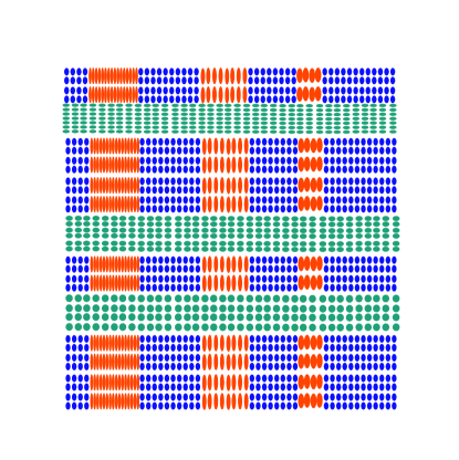
Figure 1: Schematic plot of one slice of the simulated tensor field.

Table 1: Description of the simulated tensor field

Band orientation	Slice #	Band #	Indices for band boundaries	Tensor on band
Horizontal	1 and 2	1	20, 35	diag$(0.25,16,0.25)$
		2	60, 75	diag$(0.5,4,0.5)$
		3	90, 105	diag$(0.7,2,0.7)$
	3 and 4	1	40, 50	diag$(0.25,16,0.25)$
		2	80, 90	diag$(0.5,4,0.5)$
		3	110, 120	diag$(0.7,2,0.7)$
Vertical	1 and 2	1	20, 35	diag$(16,0.25,0.25)$
		2	60, 75	diag$(4,0.5,0.5)$
		3	90, 105	diag$(2,0.7,0.7)$
	3 and 4	1	40, 50	diag$(0.25,16,0.25)$
		2	80, 90	diag$(0.5,4,0.5)$
		3	110, 120	diag$(0.7,2,0.7)$

3.2 Noise models

After the tensors (referred to as the true tensors) are simulated according to the previous section, we add noise to them to derive noise corrupted tensors (referred to as the observed tensors). We consider two different noise structures. The first noise model is motivated by the process of data acquisition in DT-MRI studies from diffusion weighted imaging data. The second noise model is motivated by the consideration of decoupling the noise variability in the eigenvalues and eigenvectors. We describe both models in detail in the following.

Rician noise

In this model, we first generate the noiseless diffusion-weighted multi-angular images (DWI) data via model (10) (Mori, 2007) using a set of $9$ gradient directions, i.e., for a voxel with true diffusion tensor $D$, the diffusion weighted signal intensity in direction $b_{k}$ (a $3\times 1$ vector of unit norm) is modeled as

$$\overline{S}_{k}=S_{0}\exp\left(-b_{k}^{T}Db_{k}\right),$$ (10)

where $S_{0}$, or the baseline signal strength (without diffusion weighting), is set to be $10$ in our simulation. These $9$ gradient directions come from a real DT-MRI study, and they are the normalized versions of the following vectors:

$$(1,0,1),~{}(1,1,0),~{}(0,1,1),~{}(0.3,0.2,0.1),~{}(0.9,0.45,0.2),~{}(1,0,0),~{}(0,1,0),~{}(0,0,1),~{}(2,1,1.3).$$

In our simulation, each of the 9 gradient directions is repeated twice which results in $18$ DWI measurements per tensor. (This is the design used in the aforementioned real study). These DWI intensities $\overline{S}_{k}$ are then corrupted by Rician noise (see equation (24) in Section 5), which gives rise to noise corrupted DWI’s $S_{k}$’s (referred to as the observed DWI’s) for each tensor. We consider three different values for the noise parameter $\sigma$ in equation (24), namely, $\sigma=0.1,0.5,1$ which corresponds to low, moderate and high noise levels, respectively. Finally, at each voxel, a regression procedure is applied to the observed DWI data to derive the observed tensor. Two different regression procedures are considered (i) linear regression of $\{\log(S_{k})\}$ on $\{b_{k}\}$ (see equation (25)); (ii) nonlinear regression of $\{S_{k}\}$ on $\{b_{k}\}$ (see equation (26)). Note that, unlike smoothing methods, for each voxel, regression procedures only use DWI data from that voxel to derive the corresponding tensor and no information from neighboring voxels is used. See Section 5 for more details on the regression procedures.

The analysis carried out in Section 5 also shows that, under the Rician noise model, at relatively high signal-to-noise ratios, the observed DWI intensities as well as the tensors derived from them by regression methods are approximately unbiased, i.e. $\mathbb{E}(S_{k})\approx\bar{S}_{k}$, and $\mathbb{E}(\widehat{D})\approx D$. A high signal-to-noise ratio results from either a small noise level for each intensity measurement (i.e., a small $\sigma$), or a large number of gradient directions. This implies that, under such cases, we can view Rician noise for tensors as an approximately additive noise (See also Remark 8 in Section 5).

Spectral noise

In this model, tensors are corrupted directly by adding random perturbations to their eigenvalues and eigenvectors which leads to a highly non-additive noise structure. Specifically, consider the spectral decomposition of the tensor $D$

$$D=E\Lambda E^{T},$$

where $\Lambda$ is a diagonal matrix with positive non-increasing diagonal elements (i.e., eigenvalues of $D$), and $E$ is the corresponding orthogonal matrix consisting of eigenvectors of $D$. Then, the noise corrupted tensor $\widetilde{D}$ is derived by

$$\widetilde{D}:=\widetilde{E}\widetilde{\Lambda}\widetilde{E}^{T}.$$

In the above, $\widetilde{\Lambda}$ is a diagonal matrix, with $\widetilde{\Lambda}_{jj}=\Lambda_{jj}U_{j}$ ($j=1,2,3$) where $U_{j}$’s are i.i.d. $\chi_{(\nu)}^{2}/\nu$. Here $\nu$ is a positive integer and $\chi_{(\nu)}^{2}$ denotes the Chi-square distribution with $\nu$ degrees of freedom. The parameter $\nu$ controls the degree of fluctuation of $\widetilde{\Lambda}$ around $\Lambda$. Indeed, $\mathbb{E}(\widetilde{\Lambda})=\Lambda$, and larger $\nu$ implies smaller fluctuations. Moreover,

$$\widetilde{E}:=(I_{3}+\eta Z)[(I_{3}+\eta Z)^{T}(I_{3}+\eta Z)]^{-1/2}E$$

where $Z$ is a $3\times 3$ matrix with i.i.d. $N(0,1)$ entries, which are independent of $\{U_{j}\}_{j=1}^{3}$, and $\eta>0$. Note that, $(I_{3}+\eta Z)[(I_{3}+\eta Z)^{T}(I_{3}+\eta Z)]^{-1/2}$ is a random orthogonal matrix. The parameter $\eta$ controls the degree of this matrix deviating from the identify matrix $I_{3}$ and larger $\eta$ implies more fluctuations in $\tilde{E}$. In the simulation, we consider the following values for the noise parameters $(\nu,\eta)$: (50,0.1), (50,0.2) (50,0.3), (20,0.1), (20,0.2) and (20,0.3).

3.3 Results of tensor smoothing

In this section, we report the estimation errors in terms of the affine-invariant distance (7) between the true and smoothed tensors at each voxel. We observe that these errors across the tensor field have a right-skewed distribution (more skewed for the geometric smoothers). Thus, measures like mean and standard deviation are not very representative of the error distribution. Therefore, the median and median absolute deviation about median (abbreviated as MAD) of the errors are used as performance measures. Median quantifies the typical error across tensors and MAD measures the robustness of the smoothers. Under the Rician noise model, for geometric smoothing, the MAD of the errors is somewhat larger than that of Euclidean smoothing, especially at higher noise levels, indicating that geometric smoothing is more sensitive to nearly additive noise. The situation is reversed for the spectral noise model.

For a clearer comparison of different smoothing methods, the tensor fields are divided into different regions and the median errors within each region are reported for different smoothers and different bandwidth choices. Six regions are considered and they are illustrated in the schematic plot Figure 2. Specifically, “whole set” refers to the whole tensor field; “bands crossing” refers to crossing of two bands and the boundary of a band and the background (tensors circles by black line in Figure 2); “background interior” refers to regions within the background which are at least four tensors away from any band (dark blue tensors); “bands interior” refers to regions within a band which are at least four tensors away from the background (red and green tensors); “background boundary” refers to regions within the background which are within four tensors away of a band (light blue tensors); and “bands boundary” refers to regions on bands which are within four tensors away from the background (orange and light green tensors). As mentioned earlier, the background consists of isotropic tensors and the bands consist of anisotropic tensors. Moreover, both “background interior” and “bands interior” are relatively homogeneous regions (i.e., the neighboring tensors are alike), whereas “background boundary”, “bands boundary” are relatively heterogeneous regions (i.e., neighboring tensors could be very different), and “bands crossing” are highly heterogeneous regions.

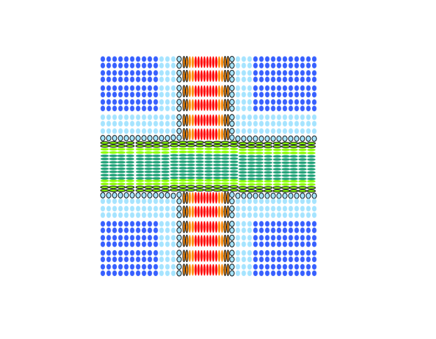
Figure 2: Schematic plot of different regions for the simulation design.

Results under Rician noise model

Three smoothers corresponding to three geometries on the tensor space are considered, namely (a) Euclidean smoothing; (b) Log-Euclidean smoothing; and (c) affine-invariant smoothing. Tensors from both linear regression of observed DWI’s (referred to as linear input) and nonlinear regression of observed DWI’s (referred to as nonlinear input) are used as inputs for tensor smoothing. We consider both the isotropic smoothing scheme and the anisotropic smoothing scheme. In the latter case, the smoothing is done in two stages. In the first stage, isotropic smoothing is performed to get a preliminary estimate $\widehat{D}_{iso}(s)$ at each voxel $s$ and in the second stage, anisotropic weights are derived by setting $\widehat{D}=\widehat{D}_{iso}(s)$ in (9) and then smoothing is performed using the isotropically smoothed tensors $\widehat{D}_{iso}(s)$’s and these weights. Three different bandwidth choices are considered for isotropic smoothing: $h=0.005$, 0.01 and 0.025. For anisotropic smoothing, the bandwidth pairs being considered are $(h_{iso},h_{aniso})=(0.005,0.01)$, $(0.01,0.01)$ and $(0.01,0.025)$, where $h_{iso}$ and $h_{aniso}$, denote the bandwidths used in the first stage and the second stage, respectively. We use a Gaussian kernel and truncate the weights that fall below a small threshold ($10^{-6}$) to speed up computation. We then re-scale the weights such that their summation equals to one. The set of neighboring voxels that receive positive weights is defined as the neighborhood. The neighborhood does not vary across tensors for isotropic smoothing at each given bandwidth, but it is varying for anisotropic smoothing. In Table 2, the size of each neighborhood, the number of voxels which account for (cumulatively) $99\%$ of the total weights (in parentheses), as well as summary statistics of the weights distribution such as minimum, median, maximum and entropy (defined as $-\sum_{i}\omega_{i}\log\omega_{i}$) for isotropic smoothing are reported. Note that, as bandwidth increases, the entropy of the weights also increases. Also note that, $h=0.005$ results in essentially no smoothing (since $>99\%$ of the weights are on the voxel under smoothing itself).

Table 2: Neighborhood size and summary statistics of the weights distribution for isotropic smoothing.

$h$	Size	min($\omega$)	median($\omega$)	max($\omega$)	Entropy($\omega$)
0.005	5 (1)	0.000881	0.000881	0.996477	0.0283
0.01	23 (9)	0.000002	0.000487	0.551461	1.5140
0.025	147 (113)	0.000061	0.002371	0.071480	4.0034

We also conduct simulations where the nine gradient directions are used only once in the DWI data generation. Table 3 reports the median and MAD of the estimation errors for linear and nonlinear regression procedures across different regions. It shows that (i) nonlinear regression of the observed DWI data gives more accurate estimate of the tensors compared to the linear regression. The improvement is only slight on the background (i.e., the isotropic regions). However, the improvement is significant on the bands (i.e., the anisotropic regions); (ii) comparison under the two simulation schemes (9 gradients each used once and twice, respectively) shows that the results for both linear and nonlinear regression improve when the number of gradient directions increases; (iii) results across different noise levels show that the performance of both linear and nonlinear regression degrades when the noise level increases.

Table 3: Comparison between linear regression and nonlinear regression on DWI data. Reported numbers are the medians of the error norms (in parenthesis, MAD of error norms) in three regions: whole set, bands and background.

gradient directions each used once
Noise level	Method	Whole set	Bands	Background
$\sigma=0.1$	linear	0.1049 (0.0460)	0.3207 (0.2409)	0.0757 (0.0185)
	nonlinear	0.0991 (0.0380)	0.1823 (0.1177)	0.0757 (0.0185)
$\sigma=0.5$	linear	0.5462 (0.2523)	1.6672 ( 1.3299)	0.3850 (0.0982)
	nonlinear	0.5141 (0.2148)	1.0617 (0.7383)	0.3829 (0.0970)
$\sigma=1$	linear	1.2382 (0.6738)	10.9 ( 5.844)	0.819 (0.2592)
	nonlinear	1.1318 (0.5615)	2.8713 (2.3365)	0.8009 (0.2424)
9 gradient directions each repeated twice
Noise level	Method	Whole set	Bands	Background
$\sigma=0.1$	linear	0.073891 (0.0322)	0.229592 (0.1734)	0.053692 (0.0130)
	nonlinear	0.069904 (0.0267)	0.129959 (0.0844)	0.053679 (0.0130)
$\sigma=0.5$	linear	0.383068 (0.1770)	1.330171 (1.0666)	0.271789 (0.0681)
	nonlinear	0.359311 (0.1481)	0.828572 (0.5926)	0.269491 (0.0672)
$\sigma=1$	linear	0.825685 (0.4091)	2.489265 (2.0479)	0.566317 (0.1579)
	nonlinear	0.758624 (0.3443)	1.726173 (1.2410)	0.548341 (0.1484)

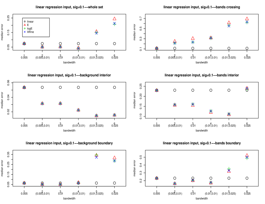
Figure 3: Rician noise with $\sigma=0.1$. Comparison of median errors over different regions for “observed” tensors (obtained by linear regression, represented by black circle) and Euclidean (red triangle), log-Euclidean (green $+$) and Affine smoothers (blue $\times$).

The median errors for different smoothers across different bandwidths within each of the six regions (illustrated by Figure 2) are plotted in Figures 3 to 8. In these figures, the $x$ axis denotes bandwidths, and the median errors for different smoothers and the observed tensors are represented by different symbols, with circle corresponding to the observed tensor (either derived by linear regression or by nonlinear regression), triangle corresponding to Euclidean smoothing, $+$ corresponding to log-Euclidean smoothing, and $\times$ corresponding to affine-invariant smoothing. The main findings are summarized below.

1. Tensor smoothing generally improves upon the corresponding regression results (either linear or nonlinear) except for the “bands crossing” regions which are highly heterogenous.

2. At small noise levels ($\sigma=0.1$), the three smoothers – Euclidean, log-Euclidean and affine-invariant – perform comparably, with geometric methods working slightly better.

3. At moderate to large noise levels ($\sigma=0.5$ or 1), the Euclidean smoother works better or even considerably better (e.g. when $\sigma=1$) than the two geometric smoothers.

4. The log-Euclidean smoother appears to be more sensitive to noise than the affine-invariant smoother indicated by a better performance of the latter under large noise levels ($\sigma=1$). Overall, the qualitative performances of these two methods are comparable.

5. Euclidean smoothing results in prominent swelling effects near the crossing of two bands.

6. At small noise levels ($\sigma=0.1$), geometric smoothing methods perform better than Euclidean smoothing in the regions with high degrees of heterogeneity, i.e., the “bands crossing” regions.

7. At comparable bandwidths, anisotropic smoothing often improves over isotropic smoothing. For example, anisotropic with $(0.01,0.01)$ performs better than isotropic with $h=0.01$ except for on “bands crossing”; and anisotropic with $(0.01,0.025)$ performs better than isotropic with $h=0.025$ at small noise levels (except for on “background boundary”).

8. In terms of bandwidths choices, in more homogeneous regions, relatively larger bandwidths are preferred, whereas in more heterogeneous regions, smaller bandwidths are preferred. Also, larger bandwidths are preferred under higher noise levels. More specifically, on “bands crossing” (highly heterogeneous), for small noise levels ($\sigma=0.1$), isotropic smoothing with $h=0.005$ is the best which indeed corresponds to nearly no smoothing, whereas, for larger noise levels ($\sigma=0.5$, 1), isotropic smoothing with $h=0.01$ is the best. On “background interior” (highly homogeneous and isotropic), anisotropic smoothing with $(0.01,0.025)$ and isotropic smoothing with $h=0.025$ work comparably and better than other bandwidth choices. On “bands interior” (relatively homogenous and highly anisotropic), anisotropic smoothing with $(0.01,0.01)$ or $(0.01,0.025)$ is the best under small noise levels, and isotropic smoothing with $h=0.025$ is the best under larger noise levels. On “bands boundary” (relatively heterogeneous), anisotropic smoothing with $(0.005,0.01)$ is the best under small noise levels, whereas isotropic smoothing with $h=0.025$ is the best under larger noise levels. On “background boundary” (relatively heterogeneous), under small noise levels, isotropic smoothing with $h=0.005$ or 0.01 and anisotropic smoothing with $(0.005,0.01)$ or $(0.01,0.01)$ all work comparably and are better than other bandwidths choices, whereas under larger noise levels, anisotropic smoothing with $(0.01,0.01)$ is the best.

Results under spectral noise

The three smoothers corresponding to Euclidean, Log-Euclidean, and affine-invariant metrics are applied to the noise corrupted tensors. Four different bandwidth choices for isotropic smoothing: $h=0.005$, $0.01$, $0.025$ and $0.035$ are considered. For anisotropic smoothing, the bandwidth pairs being considered are $(h_{iso},h_{aniso})=(0.005,0.01)$ and $(0.01,0.025)$.

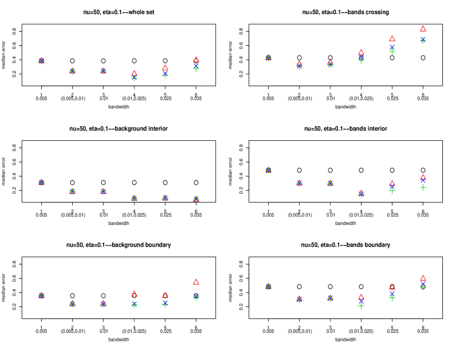
Figure 9: Spectral noise with $\nu=50$ and $\eta=0.1$. Comparison of median errors over different regions for observed tensors (black circle) and Euclidean (red triangle), log-Euclidean (green $+$) and Affine smoothers (blue $\times$).

The median errors are plotted in Figures 9 to 14. The main findings are summarized below.

1. At all noise levels, the geometric smoothers outperform the Euclidean smoother across all regions except for “background interior” (highly homogeneous and isotropic) where Euclidean smoother works slightly better under larger noise levels $(\nu=20)$.

2. Log-Euclidean smoother performs slightly better than the affine-invariant smoother, even though their qualitative performances are comparable.

3. Euclidean smoother results in prominent swelling effects near the crossing of two bands.

4. Geometric smoothing are more advantageous in the regions that are more heterogeneous. This can be seen by comparing the results on “background boundary” with “background interior”, and “bands boundary” with “bands interior”.

5. Anisotropic smoothing performs better than isotropic smoothing (at a comparable bandwidth and especially under smaller noise levels) in the regions with higher degrees of anisotropy. This is prominent in the regions “bands boundary” and “bands interior” (which together form the bands).

6. In terms of bandwidths choices, in more homogeneous regions, relatively larger bandwidths are preferred, whereas in more heterogeneous regions, smaller bandwidths are preferred. Also, larger bandwidths are preferred under higher noise levels. More specifically, on “bands crossing” (highly heterogeneous), anisotropic with $(0.005,0.01)$ and isotropic smoothing with $h=0.01$ work best; on “background interior” (highly homogeneous and isotropic), anisotropic smoothing with (0.01,0.025), and isotropic smoothing with $h=0.025,0.035$ work comparably and better than other bandwidths choices. On both “bands interior” (relatively homogenous and highly anisotropic), and “bands boundary” (relatively heterogeneous and highly anisotropic), anisotropic smoothing with (0.01, 0.025) works best. On “background boundary” (relatively heterogeneous), under smaller noise levels $(\nu=50)$, anisotropic smoothing with $(0.005,0.01)$ and $(0.01,0.025)$, and isotropic smoothing with $h=0.01$ work comparably and better than other bandwidths, whereas, under larger noise levels $(\nu=20)$, anisotropic smoothing with $(0.01,0.025)$ works best.

7. As $\eta$ increases (corresponding to more variable eigenvectors), for any given $\nu$, the performances of all smoothers across all regions degrade, except for the “background interior” regions (highly homogeneous and isotropic).

4 Perturbation analysis of smoothing methods

In this section, we conduct a perturbation analysis to compare the means of a set of tensors with respect to the Euclidean, log-Euclidean and Affine invariant metrics. Arsigny et al. (2005) also carry out a theoretical analysis studying and comparing log-Euclidean and affine-invariant metrics in tensor computation. They derive an asymptotic expression of the difference between the log-Euclidean mean and the affine-invariant mean when the true tensors lie in a small neighborhood of the identity matrix. They also explore situations where these two means are equal.

We carry out a perturbation analysis by adopting a framework similar to that in Arsigny et al. (2005). However, we focus mainly on the quantitative aspects of the differences between these means. In particular, we derive asymptotic expansions for the difference between the Euclidean and log-Euclidean means, and that between the Euclidean and affine-invariant means. We derive these results for general tensors, i.e., without requiring them to be nearly isotropic. These results also highlight the distinction between the situations when the noise structure is additive (meaning that the expectation of the tensors equals to the underlying noiseless tensor) and when the noise structure is non-additive.

Suppose that we observe random tensors $\{S(\omega)\in\mathcal{P}_{N}:\omega\in\Omega\}$, where $\Omega$ is an arbitrary index set with a Borel $\sigma$-algebra. Let $\mathbb{P}$ be a probability measure on $\Omega$.

Let $\bar{S}$ denote the expectation of $S(\omega)$ with respect to $\mathbb{P}$, i.e.,

$$\bar{S}:=\mathbb{E}(S)=\int S(\omega)d\mathbb{P}(\omega),$$ (11)

where the integration is defined through (ordinary) matrix addition of the tensors. Let $B(\omega):=S(\omega)-\bar{S}$. Then $\mathbb{E}(B)=\mathbf{0}$, where $\mathbf{0}$ denotes the $N\times N$ zero matrix.

Observe that, the expectation of $S(\omega)$ coincides with the weighted Karcher mean of $S(\omega)$ with respect to the Euclidean metric, i.e.,

$$\bar{S}=\mathbb{E}(S)=\arg\min_{K\in{\cal P}_{N}}\int d^{2}(K,S(\omega))dP(\omega),$$

where $d(\cdot,\cdot)$ is a Euclidean distance. Next, let $\bar{S}_{LE}$ denote the mean of $S(\omega)$ with respect to the log-Euclidean metric, i.e.,

$$\bar{S}_{LE}:=\arg\min_{K\in{\cal P}_{N}}\int d_{LE}^{2}(K,S(\omega))dP(\omega).$$ (12)

It is easy to show that,

$$\log\bar{S}_{LE}=\mathbb{E}(\log S)=\int\log S(\omega)dP(\omega).$$

Finally, let $\bar{S}_{Aff}$ denote the affine-invariant mean of $S(\omega)$, i.e.,

$$\bar{S}_{Aff}:=\arg\min_{K\in{\cal P}_{N}}\int d_{Aff}^{2}(K,S(\omega))dP(\omega),$$ (13)

In general, there is no closed form expression for $\bar{S}_{Aff}$, but $\bar{S}_{Aff}$ satisfies the following barrycentric equation (Arsigny et al., 2005):

$$\mathbb{E}(\log(\bar{S}_{Aff}^{-1/2}S\bar{S}_{Aff}^{-1/2}))=\mathbf{0}.$$ (14)

In the following, we adopt a matrix perturbation analysis approach to study the differences among means under different metrics. Let $\lambda_{j}$ denote the $j$-th largest distinct eigenvalue of $\bar{S}$ and let $P_{j}$ denote the corresponding eigen-projection. We make a distinction between the cases when $\bar{S}$ is a multiple of the identity (i.e., $\bar{S}$ is isotropic) and when otherwise (i.e., $\bar{S}$ is anisotropic). Let

$$C:=\begin{cases}\max\{\max_{j}\lambda_{j}^{-1},\max_{k\neq j}|\lambda_{k}-\lambda_{j}|^{-1}\},&\mbox{if}~{}\bar{S}\neq\lambda_{1}I\\ \lambda_{1}^{-1}&\mbox{if}~{}\bar{S}=\lambda_{1}I\\ \end{cases}$$

where $k\neq j$ corresponding to pairs of distinct eigenvalues of $\bar{S}$ and $I$ denotes the $N\times N$ identity matrix. We also assume that the probability measure $\mathbb{P}$ satisfies

$$\mathbb{P}(\sup_{\omega\in\Omega}\parallel B(\omega)\parallel<C^{-1}t)=1,$$ (15)

for some $t>0$, where $\parallel\cdot\parallel$ denotes the operator norm. Note that, $t$ can be viewed as a scale parameter indicating the spread of $S(\omega)$’s. A small value of $t$ means that the tensors are more homogeneous.

In the case that $\bar{S}$ is not a multiple of the identity (i.e., $\bar{S}$ is anisotropic), define $H_{j}$ to be the matrix

$$H_{j}:=\sum_{k\neq j}\frac{1}{\lambda_{k}-\lambda_{j}}P_{k}.$$ (16)

Note that $H_{j}P_{j}=P_{j}H_{j}=\mathbf{0}$ for all $j$. For simplicity of exposition, in the following, we consider only two cases: (a) when the eigenvalues of $\bar{S}$ are all distinct; and (b) when $\bar{S}$ is isotropic, i.e., all its eigenvalues are equal to $\lambda_{1}$.

Comparison of Euclidean and log-Euclidean means

Proposition 1

Suppose that the tensors $\{S(\omega):\omega\in\Omega\}$ and the probability distribution $\mathbb{P}$ satisfy (15).

• If the eigenvalues of $\bar{S}=\mathbb{E}(S)$ are all distinct, then

  $$\log\bar{S}_{LE}-\log\bar{S}$$ (17)

  $$= -\sum_{j=1}^{N}\frac{1}{\lambda_{j}}\mathbb{E}[\mbox{tr}(P_{j}BH_{j}B)]P_{j}-\frac{1}{2}\sum_{j=1}^{N}\frac{1}{\lambda_{j}^{2}}\mathbb{E}[\mbox{tr}(P_{j}B)]^{2}P_{j}$$

  $$+\sum_{j=1}^{N}\log\lambda_{j}\mathbb{E}\left[P_{j}BH_{j}BH_{j}+H_{j}BP_{j}BH_{j}+H_{j}BH_{j}BP_{j}\right.$$

  $$\left.-P_{j}BP_{j}BH_{j}^{2}-P_{j}BH_{j}^{2}BP_{j}-H_{j}^{2}BP_{j}BP_{j}\right]$$

  $$-\sum_{j=1}^{N}\frac{1}{\lambda_{j}}\mathbb{E}[\mbox{tr}(P_{j}B)(P_{j}BH_{j}+H_{j}BP_{j})]+O(t^{3}).$$

• If $\bar{S}=\lambda_{1}I$, then

  $$\log\bar{S}_{LE}-\log\bar{S}=-\frac{1}{2\lambda_{1}^{2}}\mathbb{E}(B^{2})+O(t^{3}).$$ (18)

Remark 1

When the eigenvalues of $\bar{S}$ are all distinct, taking trace on both sides of (17), and using the fact that $P_{j}H_{j}=\mathbf{0}$ and $P_{j}^{2}=P_{j}$, we get

$$\mbox{tr}(\log\bar{S}_{LE})-\mbox{tr}(\log\bar{S}) = -\sum_{j=1}^{N}\frac{1}{\lambda_{j}}\mathbb{E}[\mbox{tr}(P_{j}BH_{j}B)]-\frac{1}{2}\sum_{j=1}^{N}\frac{1}{\lambda_{j}^{2}}\mathbb{E}[\mbox{tr}(P_{j}B)]^{2}+O(t^{3}).$$ (19)

Since

$$\mbox{tr}(\log\bar{S}_{LE})-\mbox{tr}(\log\bar{S})=\log\det(\bar{S}_{LE})-\log\det(\bar{S}),$$

where $\det$ denotes the determinant, (19) actually gives an expansion of the determinant of $\bar{S}_{LE}$ around the determinant of $\bar{S}$.

Comparison of Euclidean and affine-invariant means

Proposition 2

Suppose that the tensors $\{S(\omega):\omega\in\Omega\}$ and the probability distribution $\mathbb{P}$ satisfy (15).

• If the eigenvalues of $\bar{S}$ are all distinct, then

  $$\log\bar{S}_{Aff}-\log\bar{S}$$ (20)

  $$= \sum_{j=1}^{N}\frac{1}{\lambda_{j}}\mbox{tr}(P_{j}(\bar{S}_{Aff}-\bar{S}))P_{j}-\sum_{j=1}^{N}\log\lambda_{j}\left(P_{j}(\bar{S}_{Aff}-\bar{S})H_{j}+H_{j}(\bar{S}_{Aff}-\bar{S})P_{j}\right)+O(t^{4})$$

  $$= -\frac{1}{2}\sum_{j=1}^{N}\frac{1}{\lambda_{j}}\mathbb{E}[\mbox{tr}(P_{j}B\bar{S}^{-1}B)]P_{j}$$

  $$~{}~{}+\frac{1}{2}\sum_{j=1}^{N}\log\lambda_{j}\mathbb{E}[P_{j}B\bar{S}^{-1}BH_{j}+H_{j}B\bar{S}^{-1}BP_{j}]+O(t^{3}).$$

• If $\bar{S}=\lambda_{1}I$, then

  $$\log\bar{S}_{Aff}-\log\bar{S}=-\frac{1}{2\lambda_{1}^{2}}\mathbb{E}(B^{2})+O(t^{3}).$$ (21)

Note that, Propositions 1 and 2 can be used together to give an asymptotic expansion for the difference between the log-Euclidean and affine-invariant means.

Remark 2

When the eigenvalues of $\bar{S}$ are all distinct, taking trace on both sides of (20), and using $P_{j}H_{j}=\mathbf{0}$, we get

$$\log\det(\bar{S}_{Aff})-\log\det(\bar{S})=\mbox{tr}(\log\bar{S}_{Aff})-\mbox{tr}(\log\bar{S})=-\frac{1}{2}\sum_{j=1}^{N}\frac{1}{\lambda_{j}}\mathbb{E}[\mbox{tr}(P_{j}B\bar{S}^{-1}B)]+O(t^{3}).$$ (22)

Remark 3

Expressions (18) and (21) show that, when $\bar{S}=\lambda_{1}I$ (i.e., isotropic), $\bar{S}_{LE}$ and $\bar{S}_{Aff}$ are the same up to the second order (in terms of the dispersion parameter $t$). On the other hand, from (17) and (20) we can conclude that when $\bar{S}$ is sufficiently far from being isotropic, there is a second order difference between $\bar{S}_{LE}$ and $\bar{S}_{Aff}$. Moreover, in these expansions, the terms involving $\log\lambda_{j}$ tend to dominate when at least one of the eigenvalues of $\bar{S}$ is close to zero. Thus, we expect to see a large difference between the log-Euclidean and affine-invariant means when $\bar{S}$ is anisotropic and has near zero eigenvalues. This is also confirmed by simulations.

Remark 4

When the noise is additive, i.e. $\bar{S}=\mathbb{E}(S)=S^{*}$ where $S^{*}$ denotes the “true” or target tensor, our analysis shows that both $\bar{S}_{Aff}$ and $\bar{S}_{LE}$ are biased “estimators” for $S^{*}$ and the bias can be quantified by Propositions 1 and 2.

Remark 5

Suppose that the noise is multiplicative in the following sense. Let $S^{*}=G\Delta G^{T}$ be the true tensor where the columns of the $N\times N$ orthogonal matrix $G$ denote the eigenvectors corresponding to the eigenvalues $\delta_{1}\geq\cdots\geq\delta_{N}>0$, which are the diagonal elements of the diagonal matrix $\Delta$. Suppose that the observed tensors are of the form

$$S(\omega)=G~{}\mbox{diag}(\delta_{1}e^{Z_{1}(\omega)},\cdots,\delta_{N}e^{Z_{N}(\omega)})G^{T}$$

where $Z_{1},\ldots,Z_{N}$ are independent random variables with $Z_{j}$ having uniform distribution on the interval $[-c_{j}t,c_{j}t]$ for constants $c_{1},\ldots,c_{N}>0$. Then, the tensors $S(\omega)$ satisfy (50) (see the proof of proposition 2). Moreover, the tensors commute with each other, which implies that $\bar{S}_{LE}=\bar{S}_{Aff}$. Now, using the fact that $\mathbb{E}(Z_{j})=0$ ($j=1,\ldots,N$), we have

$$\bar{S}_{LE} = \exp(G~{}\mbox{diag}(\mathbb{E}(\log\delta_{1}+Z_{1}),\cdots,\mathbb{E}(\log\delta_{N}+Z_{N}))G^{T})$$

$$= \exp(G\log\Delta G^{T})=G\Delta G^{T}=S^{*}.$$

However, $\mathbb{E}(e^{Z_{j}})=(e^{c_{j}t}-e^{-c_{j}t})/(2c_{j}t)\neq 1$, which implies that $\bar{S}\neq S^{*}$. In this case, the Euclidean mean will be a biased estimator for the true tensor $S^{*}$, and the bias is of the order $O(t^{2})$.

5 Regression analysis of DWI data under Rician noise model

In this section, we study the Rician noise model for diffusion weighted imaging data (Hanh et al., 2006). Our goal is to compare two regression procedures for deriving diffusion tensors from raw diffusion weighted images under this noise model.

In DT-MRI studies, the raw data obtained by MRI scanning are complex numbers representing the Fourier transformation of a magnetization distribution of a tissue at a certain point in time (cf. Mori, 2007). If the electronic noise in the real and imaginary parts of the raw data are assumed to be independent Gaussian random variables (Henkelman 1985; Gudbjartsson and Patz 1995; Macorski 1996), then the corresponding signal intensities follow a Rician distribution. Statistical properties of this noise model are studied by Zhu et al. (2009), where diagnostic tools to assess the quality of MR images are developed. Zhu et al. (2007) propose a semiparametric model for noise in diffusion-weighted images, and develop a weighted least squares estimate of the tensors. They study the effects of noise on the estimated diffusion tensors, as well as on their eigen-structures and morphological classification. The Rician noise model is also analyzed by Polzehl and Tabelow (2008) where a weighted version of the maximum likelihood estimator of the tensors is proposed.

In this section, we consider the Rician noise model and focus on: (i) obtaining asymptotic expansions of the linear and nonlinear least squares estimators in high signal-to-noise ratio (SNR) regimes – the results show that the linear regression estimate is less efficient; and (ii) showing that the nonlinear least squares estimator is asymptotically as efficient as the maximum likelihood estimator in high SNR regimes; (iii) quantifying the bias in the linear least squares estimator at low SNR. Here we assume that the gradient directions in the MR data acquisition step is fixed and the noise level varies. In contrast, in Zhu et al. (2007, 2009), the number of gradient directions increases to infinity while the noise level is kept fixed.

5.1 Rician noise model and regression estimates

We first describe the Rician noise model for diffusion-weighted MR images at a given voxel. Let $\mathcal{B}$ denote a set of gradient directions ($3\times 1$ vectors of unit norm). Under the model for diffusion tensors (cf. Mori, 2007), the noiseless diffusion weighted signal at direction $b\in\mathcal{B}$ is given by

$$\overline{S}_{b}=S_{0}\exp(-b^{T}Db),$$ (23)

where $S_{0}$ is the baseline intensity, and $D$ is a $3\times 3$ positive definite matrix (the diffusion tensor). The Rician noise model says that, the observed diffusion weighted signal $S_{b}$ is a random variable obtained by:

$$S_{b}=\left(|\overline{S}_{b}u_{b1}+\sigma\varepsilon_{b1}|^{2}+|\overline{S}_{b}u_{b2}+\sigma\varepsilon_{b2}|^{2}\right)^{1/2}=\parallel\overline{S}_{b}u_{b}+\sigma\varepsilon_{b}\parallel,$$ (24)

where $u_{b}:=(u_{b1},u_{b2})^{T}$ is a unit vector in $\mathbb{R}^{2}$, and the random vectors $\varepsilon_{b}:=(\varepsilon_{b1},\varepsilon_{b2})^{T}$ are distributed as $N(0,I_{2})$ and are assumed to be independent for different $b$. The parameter $\sigma>0$ controls the noise level.

We consider two regression based methods for estimating $D$ based on the observed DWI signal intensities $\{S_{b}:b\in\mathcal{B}\}$. For simplicity, throughout this section, $S_{0}$ is assumed to be known and fixed. The first method is to use the log transformed DWI’s to estimate $D$ by a linear regression. The resulting estimator is referred to as the linear regression estimator and denoted by $\widehat{D}_{LS}$. The second method uses nonlinear regression based on the original DWI’s to estimate $D$. The resulting estimator is referred to as the nonlinear regression estimator and denoted by $\widehat{D}_{NL}$.

In order to define these estimators, we introduce some notations. Specifically, the tensor $D$ is treated as a $6\times 1$ vector with elements $D_{11},D_{22},D_{33},D_{12},D_{13},D_{23}$. Under this notation, the quadratic form $b^{T}Db$ (where $D$ is a matrix) can be rewritten as $x_{b}^{T}D$ (where $D$ is a vector) with $x_{b}=(b_{1}^{2},b_{2}^{2},b_{3}^{2},2b_{1}b_{2},2b_{1}b_{3},2b_{2}b_{3})^{T}$. In the following, we also assume that the matrix $\sum_{b\in{\cal B}}x_{b}x_{b}^{T}$ is well-conditioned, which is guaranteed by an appropriate choice of the gradient directions. Then the linear regression and non-linear regression estimators are defined as

$$\widehat{D}_{LS}:=\arg\min_{D}\sum_{b\in{\cal B}}(\log S_{b}-\log S_{0}+x_{b}^{T}D)^{2},$$ (25)

and

$$\widehat{D}_{NL}:=\arg\min_{D}\sum_{b\in{\cal B}}(S_{b}-S_{0}\exp(-x_{b}^{T}D))^{2}.$$ (26)

Note that, these estimators are used in the simulation studies under the Rician noise model (Section 3) to derive the observed tensor at each voxel, which is then used as input for the smoothing methods.

In the following subsections, we analyze the behavior of the above estimators by varying the noise level, i.e., $\sigma$, which corresponds to varying signal-to-noise ratio (SNR). Consistency of the estimators is established under the $\sigma\to 0$ setting, i.e., the “large SNR” scenario. In addition, we also compare the nonlinear regression estimator with the maximum likelihood estimator which utilizes the Rician noise model explicitly. Throughout, we shall use $D^{0}$ to denote the true diffusion tensor.

5.2 Asymptotic analysis of $\widehat{D}_{LS}$ and $\widehat{D}_{NL}$ under large SNR

In this subsection, we carry out asymptotic expansions of the estimates $\widehat{D}_{LS}$ and $\widehat{D}_{NL}$ assuming that the noise level $\sigma$ goes to zero, while $\overline{S}_{b}$’s are treated as fixed. Effectively, this means that, $\sigma\ll\min_{b\in{\cal B}}\overline{S}_{b}$, which is equivalent to assuming that $S_{0}\gg\sigma$ and that $\max_{b\in{\cal B}}x_{b}^{T}D^{0}$ is “not too large”. Clearly, the last condition holds if the largest eigenvalue of the tensor $D^{0}$ is not very large (note that, the gradient directions are normalized to have unit norm).

Asymptotic expansion of $\widehat{D}_{LS}$

Proposition 3

As $\sigma\to 0$, $\widehat{D}_{LS}=D^{0}+\sigma D_{1,LS}+\sigma^{2}D_{2,LS}+O_{P}(\sigma^{3})$ where the random vectors $D_{1,LS}$ and $D_{2,LS}$ are given by

$$D_{1,LS}=-(\sum_{b\in{\cal B}}x_{b}x_{b}^{T})^{-1}(\sum_{b\in{\cal B}}\frac{1}{\overline{S}_{b}}(u_{b}^{T}\varepsilon_{b})x_{b}),$$ (27)

and

$$D_{2,LS}=-\frac{1}{2}(\sum_{b\in{\cal B}}x_{b}x_{b}^{T})^{-1}(\sum_{b\in{\cal B}}\frac{1}{\overline{S}_{b}^{2}}((v_{b}^{T}\varepsilon_{b})^{2}-(u_{b}^{T}\varepsilon_{b})^{2})x_{b}).$$ (28)

Remark 6

$D_{1,LS}$ has a normal distribution with mean zero and variance

$$\mbox{Var}(D_{1,LS})=(\sum_{b\in{\cal B}}x_{b}x_{b}^{T})^{-1}(\sum_{b\in{\cal B}}{\overline{S}_{b}}^{-2}x_{b}x_{b}^{T})(\sum_{b\in{\cal B}}x_{b}x_{b}^{T})^{-1},$$ (29)

whereas $D_{2,LS}$ is a weighted sum of differences of independent $\chi_{(1)}^{2}$ random variables, and hence it also has mean 0. These show that the bias in $\widehat{D}_{LS}$ is of the order $O(\sigma^{3})$.

Asymptotic expansion of $\widehat{D}_{NL}$

Unlike $\widehat{D}_{LS}$, there is no explicit expression for $\widehat{D}_{NL}$. Instead, it satisfies the normal equation:

$$\sum_{b\in{\cal B}}(S_{b}-S_{0}\exp(-x_{b}^{T}\widehat{D}_{NL}))S_{0}\exp(-x_{b}^{T}\widehat{D}_{NL})x_{b} = 0.$$ (30)

We have the following result.

Proposition 4

As $\sigma\to 0$, $\widehat{D}_{NL}=D^{0}+\sigma D_{1,NL}+\sigma^{2}D_{2,NL}+O_{P}(\sigma^{3})$, where

$$D_{1,NL}=-(\sum_{b\in{\cal B}}\overline{S}_{b}^{2}x_{b}x_{b}^{T})^{-1}(\sum_{b\in{\cal B}}\overline{S}_{b}(u_{b}^{T}\varepsilon_{b})x_{b}),$$ (31)

and

$$D_{2,NL}=(\sum_{b\in{\cal B}}\overline{S}_{b}^{2}x_{b}x_{b}^{T})^{-1}\left[\sum_{b\in{\cal B}}\overline{S}_{b}^{2}(x_{b}^{T}D_{1,NL})^{2}x_{b}+\frac{1}{2}\sum_{b\in{\cal B}}(\overline{S}_{b}x_{b}^{T}D_{1,NL}+u_{b}^{T}\varepsilon_{b})^{2}x_{b}-\frac{1}{2}\sum_{b\in{\cal B}}\parallel\varepsilon_{b}\parallel^{2}x_{b}\right].\\$$ (32)

Remark 7

$D_{1,NL}$ has a normal distribution with mean zero and variance

$$\mbox{Var}(D_{1,NL})=(\sum_{b\in{\cal B}}\overline{S}_{b}^{2}x_{b}x_{b}^{T})^{-1},$$ (33)

and $D_{2,NL}$ is a weighted sum of (dependent) $\chi^{2}_{(1)}$ random variables, with mean

$$\mathbb{E}(D_{2,NL})=-\frac{1}{2}(\sum_{b\in{\cal B}}\overline{S}_{b}^{2}x_{b}x_{b}^{T})^{-1}\left[\sum_{b\in{\cal B}}\left(1-\overline{S}_{b}^{2}x_{b}^{T}(\sum_{b^{\prime}\in{\cal B}}\overline{S}_{b^{\prime}}^{2}x_{b^{\prime}}x_{b^{\prime}}^{T})^{-1}x_{b}\right)x_{b}\right].$$ (34)

Observe that in (34), the coefficients of all the $x_{b}$’s, are negative and thus the mean of $D_{2,NL}$ is non-vanishing. Therefore, the bias in $\widehat{D}_{NL}$ is of order $O(\sigma^{2})$.

Remark 8

Propositions 3 and 4 show that, under the Rician noise model, at relatively high SNR, both linear and nonlinear regression estimators of the diffusion tensor are nearly unbiased. This means that under such a scenario, when the regression estimators are used as input for the smoothing methods, the corresponding noise structure is nearly additive.

Comparison of $\widehat{D}_{LS}$ and $\widehat{D}_{NL}$

It is clear from the above expansions that both $\widehat{D}_{LS}$ and $\widehat{D}_{NL}$ are consistent estimators when $\sigma$ goes to zero, where $\widehat{D}_{LS}$ has a bias of order $O(\sigma^{3})$ and that in $\widehat{D}_{NL}$ is of order $O(\sigma^{2})$. Up to the first order, both estimators have Gaussian fluctuations, and up to the second order, they become weighted sums of Gaussian and chi-squared random variables. The asymptotic analysis also points to an important advantage of $\widehat{D}_{NL}$ over $\widehat{D}_{LS}$: the former has a smaller asymptotic variance than the latter. That is,

$$(\sum_{b\in{\cal B}}\overline{S}_{b}^{2}x_{b}x_{b}^{T})^{-1}\preceq(\sum_{b\in{\cal B}}x_{b}x_{b}^{T})^{-1}(\sum_{b\in{\cal B}}{\overline{S}_{b}}^{-2}x_{b}x_{b}^{T})(\sum_{b\in{\cal B}}x_{b}x_{b}^{T})^{-1}$$ (35)

where $\preceq$ denotes the inequality between positive semi-definite matrices. This can be proved by using Schur complement and noticing that the matrix

$$\begin{bmatrix}\overline{S}_{b}^{2}x_{b}x_{b}^{T}&x_{b}x_{b}^{T}\\ x_{b}x_{b}^{T}&\overline{S}_{b}^{-2}x_{b}x_{b}^{T}\\ \end{bmatrix}$$

is positive semi-definite for each $b\in{\cal B}$. Indeed, the difference between the two asymptotic covariance matrices can be quite substantial if some $\overline{S}_{b}$’s are significantly smaller than $(1/|\mathcal{B}|)\sum_{b\in\mathcal{B}}\overline{S}_{b}$. This situation can arise when the true diffusion tensor $D^{0}$ has a strong directional component (i.e., being a highly anisotropic tensor). This is because, under such a situation, only a few gradient directions are likely to be aligned to the leading eigen-direction, which results in small $\overline{S}_{b}$, whereas other gradient directions lead to large $\overline{S}_{b}$. Consequently, $\widehat{D}_{LS}$ will have a high degree of variability and the quadratic forms $b^{T}Db$ associated with the gradient directions that are partially aligned to the leading eigen-direction will be poorly estimated. This fact has also been empirically verified through simulation studies (results not reported here).

5.3 Comparison of MLE and $\widehat{D}_{NL}$ under large SNR

The probability density function of the Rician noise distribution with signal parameter $\zeta$ (representing the amplitude of the signal) and noise parameter $\sigma$ is given by (cf. Polzehl and Tabelow, 2008)

$$p_{\zeta,\sigma}(x)=\frac{x}{\sigma^{2}}\exp\left(-\frac{x^{2}+\zeta^{2}}{2\sigma^{2}}\right)I_{0}\left(\frac{x\zeta}{\sigma^{2}}\right)\mathbf{1}(x>0),$$ (36)

where $I_{0}$ denotes the zero-th order modified Bessel function of the first kind. Under the Rician noise model (23) and (24), the measurements $S_{b}$’s are independent with p.d.f. $p_{\zeta(D^{0},b),\sigma}$, where $D^{0}$ is the true tensor and

$$\zeta(D,b):=S_{0}\exp(-x_{b}^{T}D)$$ (37)

so that $\overline{S}_{b}=\zeta(D^{0},b)$.

We first compute the Fisher information matrix for the Rician noise model with respect to $D$. In the following, for simplicity, $\sigma$ is treated as known.

Proposition 5

Under model (23) and (24), for a given $\sigma>0$, the Fisher information matrix with respect to $D$ at $D^{0}$ based on the data $\{S_{b}:b\in{\cal B}\}$, is

$${\cal I}(D^{0};\sigma) := \sum_{b\in{\cal B}}\mathfrak{I}(\zeta(D^{0},b);\sigma)(\zeta(D^{0},b))^{2}x_{b}x_{b}^{T}$$ (38)

$$= \sum_{b\in{\cal B}}\mathfrak{I}(\overline{S}_{b};\sigma)\overline{S}_{b}^{2}x_{b}x_{b}^{T}$$

Here $\mathfrak{I}(\zeta;\sigma)$ is the Fisher information for the parameter $\zeta$ of the Rician distribution (36), and it can be expressed as

$$\mathfrak{I}(\zeta;\sigma)=\frac{1}{\sigma^{2}}\left[e^{-\frac{\zeta^{2}}{2\sigma^{2}}}V\left(\frac{\zeta}{\sigma}\right)-\frac{\zeta^{2}}{\sigma^{2}}\right],$$ (39)

where, for $w>0$,

$$V(w):=\int_{0}^{\infty}u^{3}\frac{(I_{1}(uw))^{2}}{I_{0}(uw)}e^{-u^{2}/2}du=\frac{1}{w^{4}}\int_{0}^{\infty}v^{3}\frac{(I_{1}(v))^{2}}{I_{0}(v)}e^{-v^{2}/(2w^{2})}dv.$$ (40)

Remark 9

There is no closed form expression for $V(w)$. However, since both $I_{1}$ and $I_{0}$ are monotone increasing $C^{\infty}$ functions with subexponential growth on $[0,\infty)$, this function can be evaluated for any given $w$ by numerical integration using an appropriate quadrature method.

Let $\widehat{D}_{ML}$ denote the maximum likelihood estimator of $D$. Then $\widehat{D}_{ML}$ satisfies the likelihood equation

$$\sum_{b\in{\cal B}}\nabla\log p_{\zeta,\sigma}(S_{b})\left|{}_{\zeta=\zeta(\widehat{D}_{ML},b)}\right.=0,$$ (41)

where $\nabla\log p_{\zeta(D,b),\sigma}(x)$ denotes the gradient of $\log p_{\zeta(D,b),\sigma}(x)$ with respect to the parameter $D$. Then, similarly as in the case of $\widehat{D}_{NL}$, it can be shown that, as $\sigma\to 0$, $\widehat{D}_{ML}=D^{0}+\sigma D_{1,ML}+o_{P}(\sigma)$, where

$$\mathbb{E}(D_{1,ML})=0,\qquad\mbox{and}\qquad\mbox{Var}(D_{1,ML})=(\sum_{b\in{\cal B}}\overline{S}_{b}^{2}x_{b}x_{b}^{T})^{-1}.$$ (42)

This implies that the asymptotic variance of $\widehat{D}_{ML}$ is $\sigma^{2}(\sum_{b\in{\cal B}}\overline{S}_{b}^{2}x_{b}x_{b}^{T})^{-1}+o(\sigma^{2})$.

It can be checked that for every fixed $\zeta$, the quantity $\sigma^{2}\mathfrak{I}(\zeta;\sigma)$ is less than 1 for all $\sigma>0$ and converges to 1 as $\sigma\to 0$. From this, it follows that

$$\sigma^{2}{\cal I}(D^{0};\sigma)\to\sum_{b\in{\cal B}}\overline{S}_{b}^{2}x_{b}x_{b}^{T}~{}~{}~{}\mbox{as}~{}~{}~{}\sigma\to 0.$$ (43)

Since $\sigma=o(1)$, by Proposition 4, we have $\widehat{D}_{NL}=D^{0}+\sigma D_{1,NL}+O_{P}(\sigma^{2})$. Using (33) and (42) it can be concluded that $\widehat{D}_{NL}$ has the same asymptotic variance as the MLE when $\sigma\to 0$. In other words, under the large SNR regime, the nonlinear regression estimator $\widehat{D}_{NL}$ is asymptotically as efficient as the MLE $\widehat{D}_{ML}$. Moreover, (43) shows that when scaled by $\sigma^{2}$, the (common) asymptotic covariance matrix of $\widehat{D}_{NL}$ and MLE is the limit of the inverse of the Fisher information matrix of $D$.

5.4 Bias in $\widehat{D}_{LS}$ under small SNR

Polzehl and Tabelow (2008) discuss in detail the issue of bias in estimating tensors from the raw DWI data. They show that the raw DWI signal $S_{b}$ is a biased estimator of $\overline{S}_{b}$ and the bias becomes larger at smaller SNR. Specifically, they derive an expression for the bias which is quoted below.

Let $B(x_{b}^{T}D^{0},\sigma):=E_{D^{0},\sigma}(S_{b})-S_{0}e^{-x_{b}^{T}D^{0}}$ denote the bias in $S_{b}$ as an estimate of $\overline{S}_{b}$ when $(D^{0},\sigma)$ is the true parameter. Then

$$B(x_{b}^{T}D^{0},\sigma)=\sqrt{\frac{\pi}{2}}\sigma L_{1/2}\left(-\frac{S_{0}^{2}e^{-2x_{b}^{T}D^{0}}}{2\sigma^{2}}\right)-S_{0}e^{-x_{b}^{T}D^{0}}$$ (44)

where $L_{1/2}(x)=e^{x/2}[(1-x)I_{0}(-x/2)-xI_{1}(-x/2)]$, and $I_{\nu}$ is the $\nu$-th order modified Bessel function of the first kind (cf. Abramowitz and Stegun, 1965).

In this subsection, we investigate the effect of the noise on $\widehat{D}_{LS}$. For simplicity, we consider an idealized framework where the “informative” gradient directions can be separated from the “noninformative” ones.

Suppose that there is a direction $b\in{\cal B}$ such that $x_{b}^{T}D^{0}$ is large in the sense that, $\overline{S}_{b}=S_{0}\exp(-x_{b}^{T}D^{0})\ll\sigma$, even though $\sigma\ll S_{0}$. In that case, the analysis presented in Section 5.2 is not valid since the Taylor expansions adopted there is not appropriate due to the explosive behavior of the higher order derivatives of the associated functionals. Instead, we consider the following approximation:

$$\log S_{b}-\log S_{0} = \log\parallel e^{-x_{b}^{T}D^{0}}u_{b}+\frac{\sigma}{S_{0}}\varepsilon_{b}\parallel$$ (45)

$$= \frac{1}{2}\log\left(\frac{\sigma^{2}}{S_{0}^{2}}\parallel\varepsilon_{b}\parallel^{2}+2\frac{\sigma}{S_{0}}e^{-x_{b}^{T}D^{0}}u_{b}^{T}\varepsilon_{b}+e^{-2x_{b}^{T}D^{0}}\right)$$

$$= \frac{1}{2}\log\left(\frac{\sigma^{2}}{S_{0}^{2}}(\parallel\varepsilon_{b}\parallel^{2}+\overline{S}_{b}^{2}/\sigma^{2})\right)+\frac{1}{2}\log\left(1+2\frac{\overline{S}_{b}}{\sigma}\frac{u_{b}^{T}\varepsilon_{b}}{\parallel\varepsilon_{b}\parallel^{2}+\overline{S}_{b}^{2}/\sigma^{2}}\right)$$

$$= -\log\left(\frac{S_{0}}{\sigma}\right)+\frac{1}{2}\log(\parallel\varepsilon_{b}\parallel^{2}+\overline{S}_{b}^{2}/\sigma^{2})+\frac{\overline{S}_{b}}{\sigma}\frac{\parallel\varepsilon_{b}\parallel}{\parallel\varepsilon_{b}\parallel^{2}+\overline{S}_{b}^{2}/\sigma^{2}}\frac{u_{b}^{T}\varepsilon_{b}}{\parallel\varepsilon_{b}\parallel}$$

$$~{}~{}~{}~{}~{}~{}~{}+O_{P}\left(\frac{\overline{S}_{b}^{2}}{\sigma^{2}}\frac{\parallel\varepsilon_{b}\parallel^{2}}{(\parallel\varepsilon_{b}\parallel^{2}+\overline{S}_{b}^{2}/\sigma^{2})^{2}}\right).$$

Under the Rician noise mode (24), $\varepsilon_{b}\sim N(0,I_{2})$, and so $\parallel\varepsilon_{b}\parallel^{2}$ has the Exponential distribution with mean 2. Moreover, the third term on the RHS of (45) has mean 0. Thus this expansion clearly indicates that under the regime where $\overline{S}_{b}\ll\sigma$, the linear regression estimator $\widehat{D}_{LS}$ will be biased .

To make the argument more concrete, we consider the scenario where the gradient set ${\cal B}$ can be partitioned into ${\cal B}_{0}\cup{\cal B}_{0}^{c}$ such that, for $b\in{\cal B}_{0}$, $\overline{S}_{b}^{-1}=o(\sigma^{-1})$ and for $b\in{\cal B}_{0}^{c}$, $\overline{S}_{b}=o(\sigma)$. Then the linear regression estimator $\widehat{D}_{LS}$ can be expressed as follows. Define $\overline{S}^{*}:=\min_{b\in{\cal B}}\overline{S}_{b}$, $\overline{S}_{*}:=\max_{b\in{\cal B}_{0}^{c}}\overline{S}_{b}$ and $\overline{S}_{**}:=\min_{b\in{\cal B}_{0}}\overline{S}_{b}$. Then,

$$\widehat{D}_{LS} = -(\sum_{b\in{\cal B}}x_{b}x_{b}^{T})^{-1}(\sum_{b\in{\cal B}}(\log S_{b}-\log S_{0})x_{b})$$

$$= (\sum_{b\in{\cal B}}x_{b}x_{b}^{T})^{-1}\left[(\sum_{b\in{\cal B}_{0}}x_{b}x_{b}^{T})D^{0}-(\sum_{b\in{\cal B}_{0}}\frac{\sigma}{\overline{S}_{b}}(u_{b}^{T}\varepsilon_{b})x_{b})\right]$$

$$+(\sum_{b\in{\cal B}}x_{b}x_{b}^{T})^{-1}\left[\log\left(\frac{S_{0}}{\sigma}\right)\sum_{b\in{\cal B}_{0}^{c}}x_{b}-\frac{1}{2}\sum_{b\in{\cal B}_{0}^{c}}\log(\parallel\varepsilon_{b}\parallel^{2}+\overline{S}_{b}^{2}/\sigma^{2})x_{b}\right.$$

$$~{}~{}~{}~{}\left.-\sum_{b\in{\cal B}_{0}^{c}}\frac{\overline{S}_{b}}{\sigma}\frac{\parallel\varepsilon_{b}\parallel}{\parallel\varepsilon_{b}\parallel^{2}+\overline{S}_{b}^{2}/\sigma^{2}}\frac{u_{b}^{T}\varepsilon_{b}}{\parallel\varepsilon_{b}\parallel}x_{b}\right]$$

$$~{}~{}~{}~{}+O_{P}\left(\max\{\left(\frac{\sigma}{\overline{S}^{*}}\right)^{2},\left(\frac{\overline{S}_{*}}{\sigma}\right)^{2}\max_{b\in{\cal B}_{0}^{c}}\frac{\parallel\varepsilon_{b}\parallel^{2}}{(\parallel\varepsilon_{b}\parallel^{2}+(\overline{S}_{**}/\sigma)^{2})^{2}}\}\right).$$

The above expression can be decomposed as the summation of the bias and variance terms up to the first order, which is more easily interpretable:

$$\widehat{D}_{LS}-D^{0} = (\sum_{b\in{\cal B}}x_{b}x_{b}^{T})^{-1}\left[-(\sum_{b\in{\cal B}_{0}^{c}}x_{b}x_{b}^{T})D^{0}+\sum_{b\in{\cal B}_{0}^{c}}(\log(\frac{S_{0}}{\sigma})-\frac{1}{2}\log(\parallel\varepsilon_{b}\parallel^{2}+\overline{S}_{b}^{2}/\sigma^{2}))x_{b}\right]$$ (46)

$$-(\sum_{b\in{\cal B}}x_{b}x_{b}^{T})^{-1}\left[\sum_{b\in{\cal B}_{0}}\frac{\sigma}{\overline{S}_{b}}(u_{b}^{T}\varepsilon_{b})x_{b}+\sum_{b\in{\cal B}_{0}^{c}}\frac{\overline{S}_{b}}{\sigma}\frac{\parallel\varepsilon_{b}\parallel}{\parallel\varepsilon_{b}\parallel^{2}+\overline{S}_{b}^{2}/\sigma^{2}}\frac{u_{b}^{T}\varepsilon_{b}}{\parallel\varepsilon_{b}\parallel}x_{b}\right]$$

$$~{}~{}~{}~{}+O_{P}\left(\max\{\left(\frac{\sigma}{\overline{S}^{*}}\right)^{2},\left(\frac{\overline{S}_{*}}{\sigma}\right)^{2}\max_{b\in{\cal B}_{0}^{c}}\frac{\parallel\varepsilon_{b}\parallel^{2}}{(\parallel\varepsilon_{b}\parallel^{2}+(\overline{S}_{**}/\sigma)^{2})^{2}}\}\right).$$

The second term on the RHS has mean zero and has the major contribution in the variability of $\widehat{D}_{LS}$, while the first term primarily contributes to its bias.

Acknowledgement

Chen, Paul and Peng’s research was partially supported by the NSF grant DMS-0806128.

Appendix

Perturbation analysis of tensor means

Proof of Proposition 1

First consider case (a): the eigenvalues of $\bar{S}$ are distinct. Let $\mu_{j}(\omega)$ denote the $j$-th largest eigenvalue of $S(\omega)$ and $Q_{j}(\omega)$ denote the corresponding eigen-projection. Then under (15), for $t$ sufficiently small, with probability 1, $\mu_{j}(\omega)$ is of multiplicity 1, and so $Q_{j}(\omega)$ is a rank 1 matrix. We can then use the following matrix perturbation analysis results:

$$\mu_{j}(\omega)=\lambda_{j}+\mbox{tr}(P_{j}B(\omega))-\mbox{tr}(P_{j}B(\omega)H_{j}B(\omega))+O(C^{2}\parallel B\parallel_{\infty}^{3}),$$ (47)

where tr denotes the trace of a matrix, and

$$Q_{j}(\omega) = P_{j}-(P_{j}B(\omega)H_{j}+H_{j}B(\omega)P_{j})$$ (48)

$$+P_{j}B(\omega)H_{j}B(\omega)H_{j}+H_{j}B(\omega)P_{j}B(\omega)H_{j}+H_{j}B(\omega)H_{j}B(\omega)P_{j}$$

$$-P_{j}B(\omega)P_{j}B(\omega)H_{j}^{2}-P_{j}B(\omega)H_{j}^{2}B(\omega)P_{j}-H_{j}^{2}B(\omega)P_{j}B(\omega)P_{j}+O(C^{3}\parallel B\parallel_{\infty}^{3}),$$

where $\parallel B\parallel_{\infty}:=\sup_{\omega\in\Omega}\parallel B(\omega)\parallel$.

In order to compare the Euclidean mean with the mean defined in terms of the log-Euclidean metric, we consider an asymptotic expansion of $\log S(\omega)$ around $\log\bar{S}$, where the asymptotics is as $t\to 0$.

By definition, and using (15), for $t$ sufficiently small,

$$\log S(\omega)-\log\bar{S}$$

$$= \sum_{j=1}^{N}(\log\mu_{j}(\omega)Q_{j}(\omega)-\log\lambda_{j}P_{j})$$

$$= \sum_{j=1}^{N}(\log\mu_{j}(\omega)-\log\lambda_{j})P_{j}+\sum_{j=1}^{N}\log\lambda_{j}(Q_{j}(\omega)-P_{j})+\sum_{j=1}^{N}(\log\mu_{j}(\omega)-\log\lambda_{j})(Q_{j}(\omega)-P_{j})$$

Now, from (47) and (15), we have

$$\log\mu_{j}(\omega)-\log\lambda_{j} = \log\left(1+\frac{\mu_{j}(\omega)-\lambda_{j}}{\lambda_{j}}\right)$$

$$= \frac{1}{\lambda_{j}}[\mbox{tr}(P_{j}B(\omega))-\mbox{tr}(P_{j}B(\omega)H_{j}B(\omega))]-\frac{1}{2\lambda_{j}^{2}}[\mbox{tr}(P_{j}B(\omega))]^{2}+O(t^{3}),$$

where we have used the series expansion $\log(1+x)=\sum_{n=1}^{\infty}(-1)^{n-1}x^{n}/n$. Substituting in (Proof of Proposition 1) and using (48), we get,

$$\log S-\log\bar{S}$$

$$= \sum_{j=1}^{N}\frac{1}{\lambda_{j}}\mbox{tr}(P_{j}B(\omega))P_{j}-\sum_{j=1}^{N}\frac{1}{\lambda_{j}}\mbox{tr}(P_{j}B(\omega)H_{j}B(\omega))P_{j}-\frac{1}{2}\sum_{j=1}^{N}\frac{1}{\lambda_{j}^{2}}[\mbox{tr}(P_{j}B(\omega))]^{2}P_{j}$$

$$-\sum_{j=1}^{N}\log\lambda_{j}[P_{j}B(\omega)H_{j}+H_{j}B(\omega)P_{j}]$$

$$+\sum_{j=1}^{N}\log\lambda_{j}\left[P_{j}B(\omega)H_{j}B(\omega)H_{j}+H_{j}B(\omega)P_{j}B(\omega)H_{j}+H_{j}B(\omega)H_{j}B(\omega)P_{j}\right.$$

$$\left.-P_{j}B(\omega)P_{j}B(\omega)H_{j}^{2}-P_{j}B(\omega)H_{j}^{2}B(\omega)P_{j}-H_{j}^{2}B(\omega)P_{j}B(\omega)P_{j}\right]$$

$$-\sum_{j=1}^{N}\frac{1}{\lambda_{j}}\mbox{tr}(P_{j}B(\omega))(P_{j}B(\omega)H_{j}+H_{j}B(\omega)P_{j})+O(t^{3}).$$

From this, we get (17) by taking expectation, and recalling that $\mathbb{E}(B)=O$.

Now consider case (b): $\bar{S}=\lambda_{1}I$. Then, from the expansion

$$\log S(\omega) = (\log\lambda_{1})I+\log\left(I+\frac{1}{\lambda_{1}}B(\omega)\right)~{}=~{}\log\bar{S}+\frac{1}{\lambda_{1}}B(\omega)-\frac{1}{2\lambda_{1}^{2}}(B(\omega))^{2}+O(C^{3}\parallel B\parallel_{\infty}^{3}),$$

we obtain (18) by taking expectation.

Proof of Proposition 2

Define,

$$L(\omega)=\log(\bar{S}_{Aff}^{-1/2}S(\omega)\bar{S}_{Aff}^{-1/2}),\qquad\omega\in\Omega.$$

Note that, (14) implies that $\mathbb{E}(L)=\mathbf{0}$. First, we show that

$$\parallel L\parallel_{\infty}:=\sup_{\omega\in\Omega}\parallel L\parallel=O(t).$$ (50)

This implies that

$$\bar{S} = \mathbb{E}(S)~{}=~{}\mathbb{E}(\bar{S}_{Aff}^{1/2}e^{L}\bar{S}_{Aff}^{1/2})$$

$$= \bar{S}_{Aff}+\bar{S}_{Aff}^{1/2}\mathbb{E}(L)\bar{S}_{Aff}^{1/2}+\frac{1}{2}\bar{S}_{Aff}^{1/2}\mathbb{E}(L^{2})\bar{S}_{Aff}^{1/2}+O(t^{3}),$$

from which we get

$$\bar{S}_{Aff}=\bar{S}-\frac{1}{2}\bar{S}^{1/2}\mathbb{E}(L^{2})\bar{S}^{1/2}+O(t^{3}),$$ (51)

where, we have used the fact that $\mathbb{E}(L)=\mathbf{0}$. Now, we express $\mathbb{E}(L^{2})$ in terms of an expectation involving $B=S-\bar{S}$. In order to do this, observe that

$$B(\omega) = S(\omega)-\bar{S}~{}=~{}\bar{S}_{Aff}^{1/2}e^{L(\omega)}\bar{S}_{Aff}^{1/2}-\bar{S}_{Aff}+\bar{S}_{Aff}-\bar{S}$$

$$= \bar{S}_{Aff}^{1/2}L(\omega)\bar{S}_{Aff}^{1/2}+\frac{1}{2}\bar{S}_{Aff}^{1/2}((L(\omega))^{2}-\mathbb{E}(L^{2}))\bar{S}_{Aff}^{1/2}+O(t^{3})$$

$$= \bar{S}^{1/2}L(\omega)\bar{S}^{1/2}+\frac{1}{2}\bar{S}^{1/2}((L(\omega))^{2}-\mathbb{E}(L^{2}))\bar{S}^{1/2}+O(t^{3}),$$

where, in the second and third steps we have used (50) and (51). Therefore, again using (50),

$$\mathbb{E}(L^{2})=\bar{S}^{-1/2}\mathbb{E}(B\bar{S}^{-1}B)\bar{S}^{-1/2}+O(t^{3}),$$ (52)

which, together with (51), leads to the representation

$$\bar{S}_{Aff}=\bar{S}-\frac{1}{2}\mathbb{E}(B\bar{S}^{-1}B)+O(t^{3}).$$ (53)

Now we are in a position to complete the proof. For case (a), using similar perturbation analysis as in the expansion of $\log S(\omega)$ around $\log\bar{S}$, and then using (53), which in particular implies that $\parallel\bar{S}_{Aff}-\bar{S}\parallel=O(t^{2})$, we obtain (20).

For case (b), since $\bar{S}=\lambda_{1}I$, from (53), and using series expansion of $\log(I+K)$, where $K$ is symmetric, (21) immediately follows.

Proof of (50)

From the fact that $\parallel B\parallel_{\infty}=O(t)$, it easily follows that $\mathbb{E}(d_{Aff}^{2}(\bar{S},S))=O(t^{2})$. Then, by definition of $\bar{S}_{Aff}$ it follows that $\mathbb{E}(d_{Aff}^{2}(\bar{S}_{Aff},S))=O(t^{2})$ which implies $\mathbb{E}(d_{Aff}(\bar{S}_{Aff},S))=O(t)$. Now, writing

$$\log(\bar{S}_{Aff}^{-1/2}S(\omega)\bar{S}_{Aff}^{-1/2})=\log(\bar{S}_{Aff}^{-1/2}\bar{S}\bar{S}_{Aff}^{-1/2}+\bar{S}_{Aff}^{-1/2}B(\omega)\bar{S}_{Aff}^{-1/2})$$

and using the Baker-Campbell-Hausdorff formula, together with the fact that $\parallel B\parallel_{\infty}=O(t)$, we conclude that

$$d_{Aff}(\bar{S}_{Aff},\bar{S})=O(t)~{}~{}\mbox{so that}~{}~{}\parallel\bar{S}_{Aff}-\bar{S}\parallel=O(t).$$

From this it is easy to deduce (50).

Rician noise model

Facts about Bessel functions

The following result about Bessel functions (cf. Abramowitz and Stegun, 1965) is crucial in proving results involving the Rician noise model.

Lemma 1

For every $\nu$, and $t\neq 0$

$$I_{\nu+1}(t)=I_{\nu-1}(t)-\frac{2\nu}{t}I_{\nu}(t)\qquad\mbox{and}\qquad I_{\nu}^{\prime}(t)=I_{\nu-1}(t)-\frac{\nu}{t}I_{\nu}(t)=I_{\nu+1}(t)+\frac{\nu}{t}I_{\nu}(t),$$ (54)

where $I_{\nu}^{\prime}(t)$ denotes the derivative of $I_{\nu}(t)$ with respect to $t$.

We list down some facts about the function

$$F(t):=\frac{I_{1}(t)}{I_{0}(t)},\qquad t\in\mathbb{R}$$ (55)

that we have used in deriving the asymptotic expansion for the MLE of $D$ in the limit $\sigma\to 0$.

1. Using (54), we have a differential equation for $F$,

   $$F^{\prime}(t)=1-\frac{1}{t}F(t)-(F(t))^{2}~{}~{}~{}\mbox{for}~{}~{}~{}t\neq 0.$$ (56)

2. $F(t)\to 1$ and $t(1-F(t))\to 1/2$ as $t\to\infty$.

3. Above facts, together with (56) imply that $tF^{\prime}(t)\to 0$ and $tF^{\prime\prime}(t)\to 0$ as $t\to\infty$.

Proof of Proposition 5 : Let $\nabla\log p_{\zeta(D,b),\sigma}(x)$ denote the gradient of $\log p_{\zeta(D,b),\sigma}(x)$ with respect to the parameter $D$. Using the chain rule of differentiation, we have

$$\nabla\log p_{\zeta(D,b),\sigma}(x)=\frac{\partial}{\partial\zeta}\log p_{\zeta,\sigma}(x)\left|{}_{\zeta=\zeta(D,b)}\right.\nabla_{D}\zeta(D,b)=\frac{\partial}{\partial\zeta}\log p_{\zeta,\sigma}(x)\left|{}_{\zeta=\zeta(D,b)}\right.\cdot(-\zeta(D,b))x_{b}.$$ (57)

It is enough therefore to find the Fisher information for $\zeta$ under the Rician noise model with parameter $(\zeta,\sigma)$ (with $\sigma$ known). Now, it follows from (54) that $I_{0}^{\prime}(t)=I_{1}(t)$. Thus,

$$\frac{\partial}{\partial\zeta}\log p_{\zeta,\sigma}(x) = -\frac{\zeta}{\sigma^{2}}+\frac{x}{\sigma^{2}}\frac{I_{1}\left(\frac{x\zeta}{\sigma^{2}}\right)}{I_{0}\left(\frac{x\zeta}{\sigma^{2}}\right)}.$$ (58)

Since $\mathbb{E}(\frac{\partial}{\partial\zeta}\log p_{\zeta,\sigma}(X))=0$, from (58) it follows that the Fisher information for $\zeta$ is given by,

$$\mathfrak{I}(\zeta;\sigma):=\mbox{Var}(\frac{\partial}{\partial\zeta}\log p_{\zeta,\sigma}(X)) = \mathbb{E}\left[\frac{X}{\sigma^{2}}\frac{I_{1}\left(\frac{X\zeta}{\sigma^{2}}\right)}{I_{0}\left(\frac{X\zeta}{\sigma^{2}}\right)}\right]^{2}-\frac{\zeta^{2}}{\sigma^{4}}$$ (59)

$$= e^{-\frac{\zeta^{2}}{2\sigma^{2}}}\int_{0}^{\infty}\left(\frac{x}{\sigma^{2}}\right)^{3}\frac{(I_{1}\left(\frac{x\zeta}{\sigma^{2}}\right))^{2}}{I_{0}\left(\frac{x\zeta}{\sigma^{2}}\right)}e^{-\frac{x^{2}}{2\sigma^{2}}}dx-\frac{\zeta^{2}}{\sigma^{4}}$$

$$= \frac{1}{\sigma^{2}}\left[e^{-\frac{\zeta^{2}}{2\sigma^{2}}}\int_{0}^{\infty}u^{3}\frac{(I_{1}(u\zeta/\sigma))^{2}}{I_{0}(u\zeta/\sigma)}e^{-u^{2}/2}du-\frac{\zeta^{2}}{\sigma^{2}}\right]$$

$$= \frac{1}{\sigma^{2}}\left[e^{-\frac{\zeta^{2}}{2\sigma^{2}}}V\left(\frac{\zeta}{\sigma}\right)-\frac{\zeta^{2}}{\sigma^{2}}\right],$$

where, $V(w)$ is given by (40).

Outline of asymptotic expansions of $\widehat{D}_{LS}$ and $\widehat{D}_{NL}$

Define, for an arbitrary tensor $D$ and arbitrary gradient direction $b$,

$$f_{b}(w,D):=\parallel S_{0}e^{-x_{b}^{T}D}u_{b}+w\parallel.$$ (60)

Then, $f_{b}(0,D^{0})=\overline{S}_{b}$ and $f_{b}(\sigma\varepsilon_{b},D^{0})=S_{b}$. We denote the partial derivatives with respect to the first and second arguments by $\nabla_{ij}f_{b}$ etc, where $1\leq i,j\leq 2$. Then,

$$\nabla_{1}f_{b}(w,D^{0})=\frac{1}{f_{b}(w,D^{0})}(\overline{S}_{b}u_{b}+w)~{}~{}\Longrightarrow~{}~{}\nabla_{1}f_{b}(0,D^{0})=\frac{1}{\overline{S}_{b}}\overline{S}_{b}u_{b}=u_{b}.$$ (61)

Now, let $v_{b}\in\mathbb{R}^{2}$ be such that $v_{b}^{T}u_{b}=0$ and $\parallel v_{b}\parallel=1$ so that $u_{b}u_{b}^{T}+v_{b}v_{b}^{T}=I_{2}$. Thus, using (61),

$$\nabla_{11}f_{b}(w,D^{0}) = \frac{1}{f_{b}(w,D^{0})}I_{2}-\frac{1}{(f_{b}(w,D^{0}))^{3}}(\overline{S}_{b}u_{b}+w)(\overline{S}_{b}u_{b}+w)^{T}$$ (62)

$$\Longrightarrow \nabla_{11}f_{b}(0,D^{0})=\frac{1}{\overline{S}_{b}}(I_{2}-u_{b}u_{b}^{T})=\frac{1}{\overline{S}_{b}}v_{b}v_{b}^{T}.$$

We also have,

$$\nabla_{2}f_{b}(0,D^{0})=-S_{0}\exp(-x_{b}^{T}D^{0})x_{b}=-\overline{S}_{b}x_{b}$$ (63)

and

$$\nabla_{22}f_{b}(0,D^{0})=S_{0}\exp(-x_{b}^{T}D^{0})x_{b}x_{b}^{T}=\overline{S}_{b}x_{b}x_{b}^{T}.$$ (64)

Proof of Proposition 3 :

$$\widehat{D}_{LS} = -(\sum_{b\in{\cal B}}x_{b}x_{b}^{T})^{-1}(\sum_{b\in{\cal B}}(\log S_{b}-\log S_{0})x_{b})$$

$$= -(\sum_{b\in{\cal B}}x_{b}x_{b}^{T})^{-1}(\sum_{b\in{\cal B}}(\log f_{b}(\sigma\varepsilon_{b},D^{0})-\log f_{b}(0,D^{0})-x_{b}^{T}D^{0})x_{b})$$

$$= D^{0}-(\sum_{b\in{\cal B}}x_{b}x_{b}^{T})^{-1}\left(\sum_{b\in B}\sigma\frac{(\nabla_{1}f_{b}(0,D^{0}))^{T}\varepsilon_{b}}{f_{b}(0,D^{0})}x_{b}\right)$$

$$-\frac{1}{2}(\sum_{b\in{\cal B}}x_{b}x_{b}^{T})^{-1}\sum_{b\in{\cal B}}\sigma^{2}\left[\frac{\varepsilon_{b}^{T}\nabla_{11}f_{b}(0,D^{0})\varepsilon_{b}}{f_{b}(0,D^{0})}-\frac{(\varepsilon_{b}^{T}\nabla_{1}f_{b}(0,D^{0}))^{2}}{(f_{b}(0,D^{0}))^{2}}\right]x_{b}+O_{P}(\sigma^{3}).$$

This, together with (61) and (62), proves Proposition 3.

Proof of Proposition 4 : From this (30), and the definition of $\widehat{D}_{NL}$, using standard arguments, it can be shown that $\parallel\widehat{D}_{NL}-D^{0}\parallel=O_{P}(\sigma)$ as $\sigma\to 0$. Then, expanding the LHS of (30) in Taylor series, we have

$$\sum_{b\in{\cal B}}\left[\sigma\varepsilon_{b}^{T}\nabla_{1}f_{b}(0,D^{0})+\frac{\sigma^{2}}{2}\varepsilon_{b}^{T}\nabla_{11}f_{b}(0,D^{0})\varepsilon_{b}-(\nabla_{2}f_{b}(0,D^{0}))^{T}(\widehat{D}_{NL}-D^{0})\right.$$

$$\left.-\frac{1}{2}(\widehat{D}_{NL}-D^{0})^{T}\nabla_{22}f_{b}(0,D^{0})(\widehat{D}_{NL}-D^{0})\right]~{}~{}~{}~{}~{}~{}~{}~{}~{}~{}$$

$$~{}~{}\cdot~{}\left(\nabla_{2}f_{b}(0,D^{0})+\nabla_{22}f_{b}(0,D^{0})(\widehat{D}_{NL}-D^{0})\right) = O_{P}(\sigma^{3}).$$

Now, changing sides and collecting terms corresponding to a given power of $\sigma$, we can express $\widehat{D}_{NL}$ as $\widehat{D}_{NL}=D^{0}+\sigma D_{1,NL}+\sigma^{2}D_{2,NL}+O_{P}(\sigma^{3})$, where

$$D_{1,NL} = (\sum_{b\in{\cal B}}\nabla_{2}f_{b}(0,D^{0})(\nabla_{2}f_{b}(0,D^{0}))^{T})^{-1}(\sum_{b\in{\cal B}}\varepsilon_{b}^{T}\nabla_{1}f_{b}(0,D^{0})\nabla_{2}f_{b}(0,D^{0}))$$

which equals (31) by virtue of (63). Next, we have

$$D_{2,NL} = (\sum_{b\in{\cal B}}\nabla_{2}f_{b}(0,D^{0})(\nabla_{2}f_{b}(0,D^{0}))^{T})^{-1}\cdot$$

$$~{}~{}\left[\frac{1}{2}\sum_{b\in{\cal B}}\left(\varepsilon_{b}^{T}\nabla_{11}f_{b}(0,D^{0})\varepsilon_{b}-D_{1,NL}^{T}\nabla_{22}f_{b}(0,D^{0})D_{1,NL}\right)\nabla_{2}f_{b}(0,D^{0})\right.$$

$$+\left.\sum_{b\in{\cal B}}(\varepsilon_{b}^{T}\nabla_{1}f_{b}(0,D^{0}))\nabla_{22}f_{b}(0,D^{0})D_{1,NL}-\sum_{b\in{\cal B}}(D_{1,NL}^{T}\nabla_{2}f_{b}(0,D^{0}))\nabla_{22}f_{b}(0,D^{0})D_{1,NL}\right].$$

Now, using (61)-(64) and (31), we can simplify the expression for $D_{2,NL}$ as

$$D_{2,NL} = (\sum_{b\in{\cal B}}\overline{S}_{b}^{2}x_{b}x_{b}^{T})^{-1}\left[\frac{3}{2}\sum_{b\in{\cal B}}\overline{S}_{b}^{2}(x_{b}^{T}D_{1,NL})^{2}x_{b}-\frac{1}{2}\sum_{b\in{\cal B}}(v_{b}^{T}\varepsilon_{b})^{2}x_{b}+\sum_{b\in{\cal B}}\overline{S}_{b}(u_{b}^{T}\varepsilon_{b})(x_{b}^{T}D_{1,NL})x_{b}\right]$$

which can be rearranged to get (32).

Figures for Rician noise model

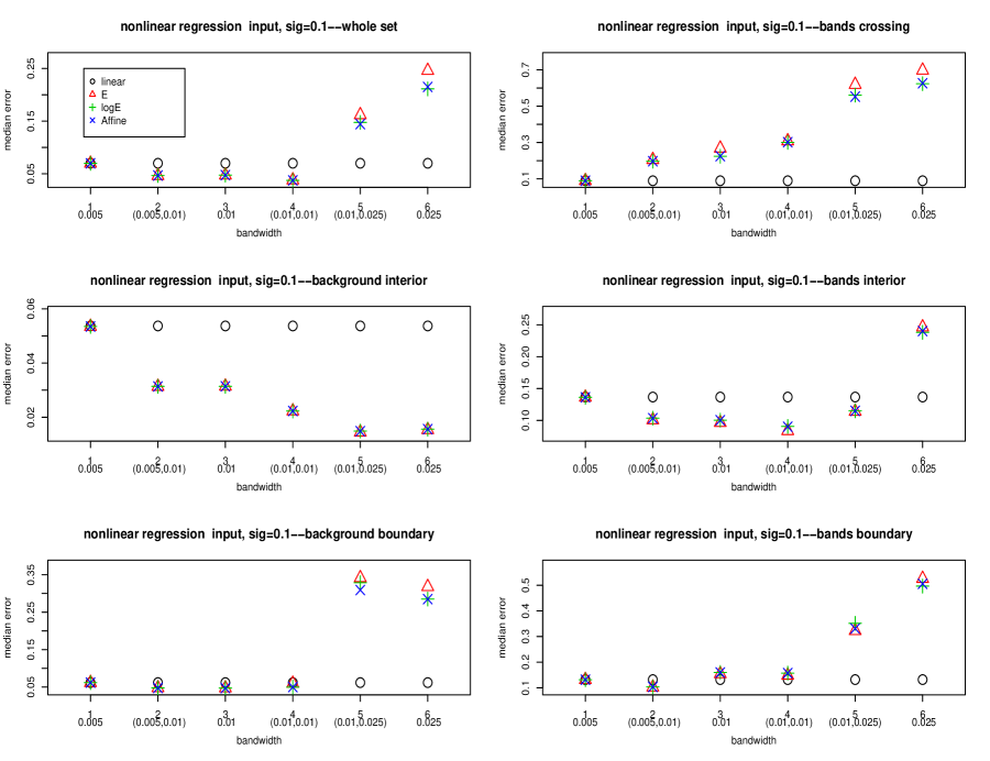
Figure 4: Rician noise with $\sigma=0.1$. Comparison of median errors over different regions for “observed” tensors (obtained by nonlinear regression, represented by black circle) and Euclidean (red triangle), log-Euclidean (green $+$) and Affine smoothers (blue $\times$).

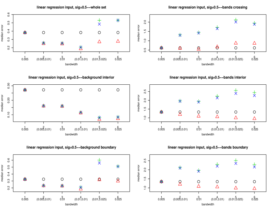
Figure 5: Rician noise with $\sigma=0.5$. Comparison of median errors over different regions for “observed” tensors (obtained by linear regression, represented by black circle) and Euclidean (red triangle), log-Euclidean (green $+$) and Affine smoothers (blue $\times$).

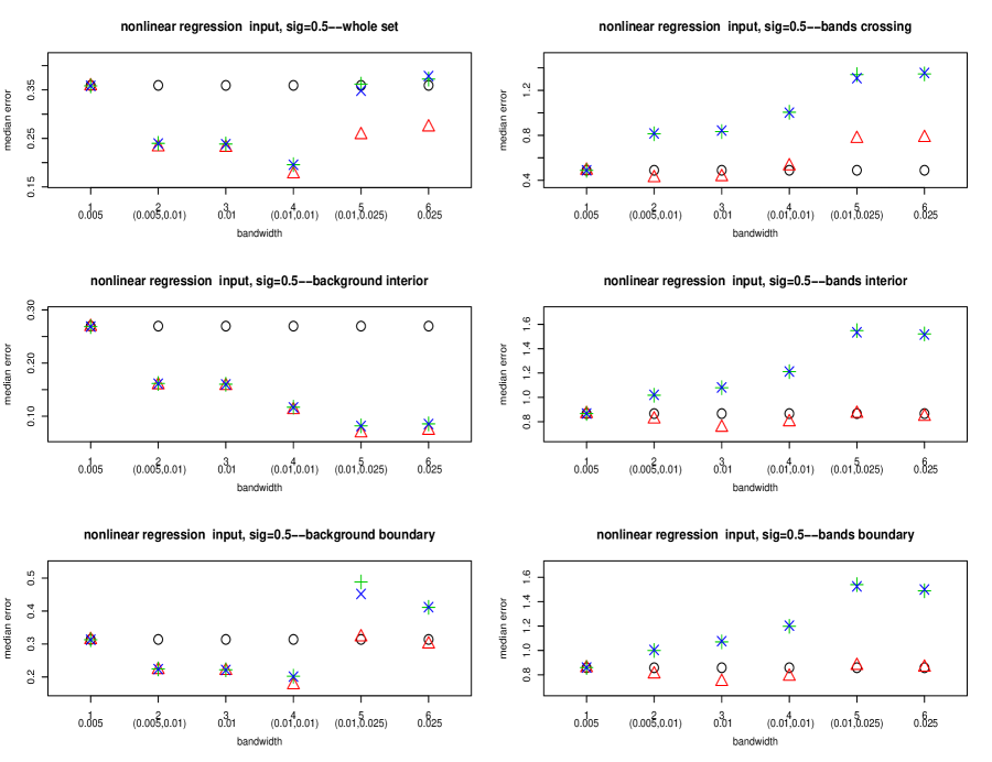
Figure 6: Rician noise with $\sigma=0.5$. Comparison of median errors over different regions for “observed” tensors (obtained by nonlinear regression, represented by black circle) and Euclidean (red triangle), log-Euclidean (green $+$) and Affine smoothers (blue $\times$).

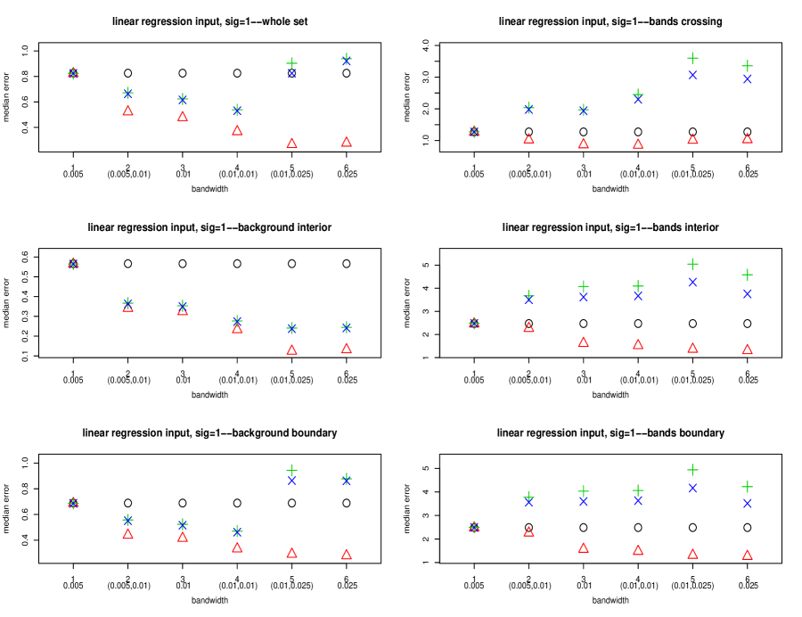
Figure 7: Rician noise with $\sigma=1$. Comparison of median errors over different regions for “observed” tensors (obtained by linear regression, represented by black circle) and Euclidean (red triangle), log-Euclidean (green $+$) and Affine smoothers (blue $\times$).

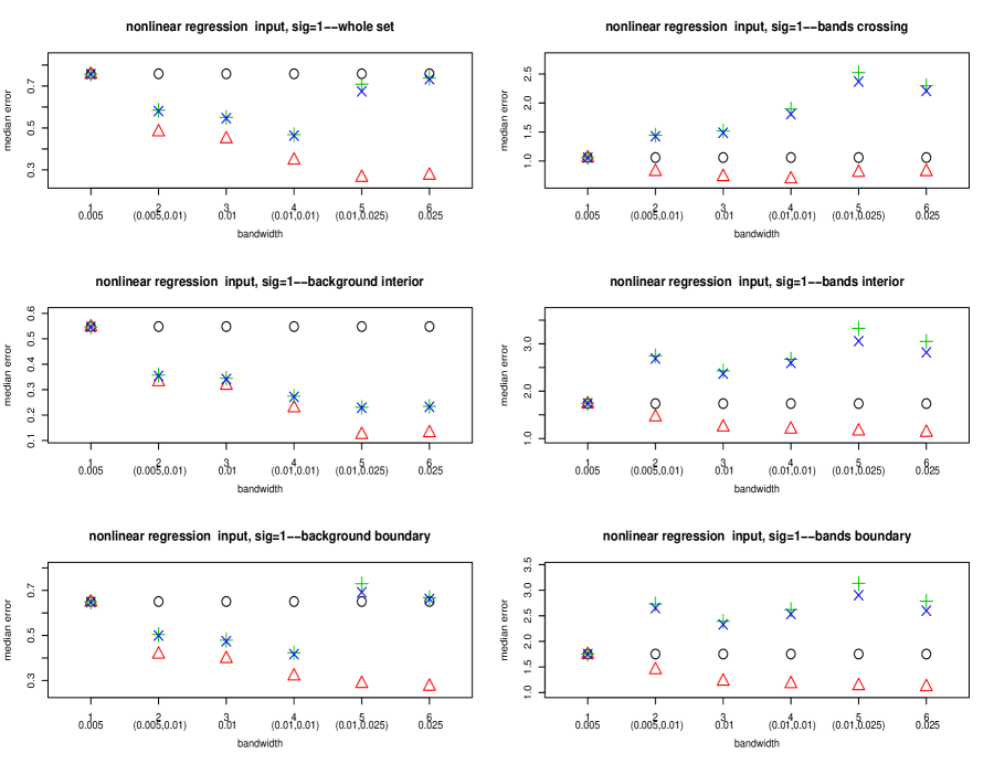
Figure 8: Rician noise with $\sigma=1$. Comparison of median errors over different regions for “observed” tensors (obtained by nonlinear regression, represented by black circle) and Euclidean (red triangle), log-Euclidean (green $+$) and Affine smoothers (blue $\times$).

Figures for spectral noise

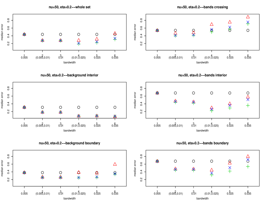
Figure 10: Spectral noise with $\nu=50$ and $\eta=0.2$. Comparison of median errors over different regions for observed tensors (black circle) and Euclidean (red triangle), log-Euclidean (green $+$) and Affine smoothers (blue $\times$).

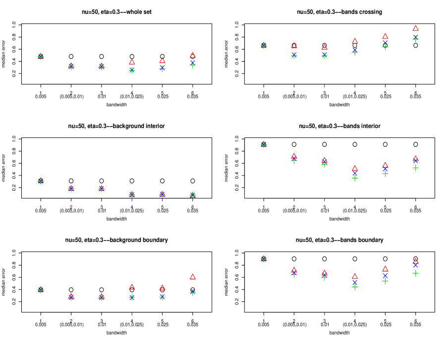
Figure 11: Spectral noise with $\nu=50$ and $\eta=0.3$. Comparison of median errors over different regions for observed tensors (black circle) and Euclidean (red triangle), log-Euclidean (green $+$) and Affine smoothers (blue $\times$).

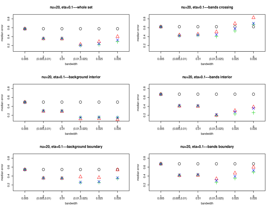
Figure 12: Spectral noise with $\nu=20$ and $\eta=0.1$. Comparison of median errors over different regions for observed tensors (black circle) and Euclidean (red triangle), log-Euclidean (green $+$) and Affine smoothers (blue $\times$).

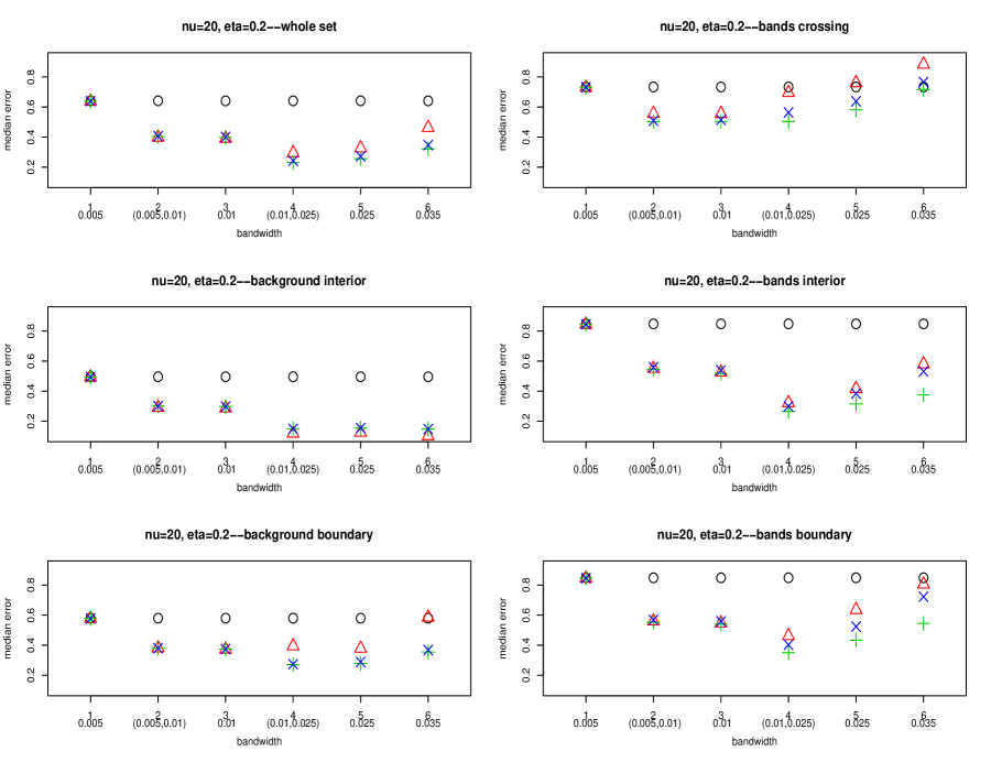
Figure 13: Spectral noise with $\nu=20$ and $\eta=0.2$. Comparison of median errors over different regions for observed tensors (black circle) and Euclidean (red triangle), log-Euclidean (green $+$) and Affine smoothers (blue $\times$).

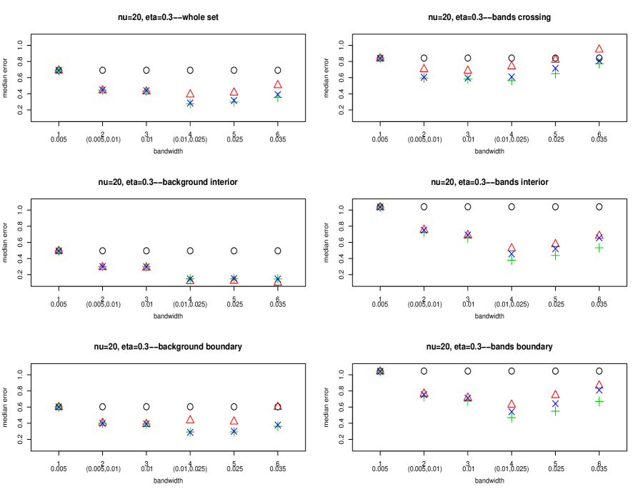
Figure 14: Spectral noise with $\nu=20$ and $\eta=0.3$. Comparison of median errors over different regions for observed tensors (black circle) and Euclidean (red triangle), log-Euclidean (green $+$) and Affine smoothers (blue $\times$).

Reference

1. Abramowitz, M. and Stegun, I. (1965). Handbook of Mathematical Functions, Ninth Edition. Dover.

2. Absil, P.-A., Mahony, R. and Sepulchre, R. (2008). Optimization Algorithms on Matrix Manifolds. Princeton University Press.

3. Arsigny, V., Fillard, P., Pennec, X. and Ayache, N. (2005). Fast and simple computations on tensors with log-Euclidean metrics. Technical report # 5584. Institut National de Recherche en Informatique et en Automatique.

4. Arsigny, V., Fillard, P., Pennec, X. and Ayache, N. (2006). Log-Euclidean metrics for fast and simple calculus on diffusion tensors. Magnetic Resonance in Medicine 56, 411-421.

5. Basser, P. and Pajevic, S. (2000). Statistical artifacts in diffusion tensor MRI (DT-MRI) caused by background noise. Magnetic Resonance in Medicine 44, 41-50.

6. Chung, M. K., Lazar, M., Alexender, A. L., Lu, Y. and Davidson, R. (2003). Probabilistic connectivity measure in diffusion tensor imaging via anisotropic kernel smoothing. Technical Report, University of Wisconsin, Madison.

7. Chung, M. K., Lee, J. E., Alexander, A. L. (2005) : Anisotropic kernel smoothing in diffusion tensor imaging : theoretical framework. Technical report, University of Wisconsin, Madison.

8. Cammoun, L., Casta o-Moraga, C. A., Muñoz-Moreno, E., Sosa-Cabrera, D., Acar, B., Rodriguez-Florido, M. A., Brun, A., Knutsson, H. and Thiran, J. P. (2009). A review of tensors and tensor signal processing. Tensors in Image Processing and Computer Vision : Advances in Pattern Recognition, Part 1, 1-32.

9. Fan, J., and Gijbels, I. (1996). Local Polynomial Modelling and Its Applications. Chapman & Hall/CRC.

10. Ferreira, R., Xavier, J., Costeira, J. P. and Barroso, V. (2006). Newton method for Riemannian centroid computation in naturally reductive homogeneous spaces. Proceedings of ICASSP 2006 - IEEE International Conference on Acoustics, Speech and Signal Processing, Toulouse, France.

11. Fletcher, P. T. and Joshi, S. (2004). Principal geodesic analysis on symmetric spaces: Statistics of diffusion tensors. In Computer Vision and Mathematical Methods in Medical and Biomedical Image Analysis, ECCV 2004 Workshops CVAMIA and MMBIA, Prague, Czech Republic, May 15, 2004, LNCS vol. 3117, 87 98. Springer.

12. Fletcher, P. T. and Joshi, S. (2007). Riemannian geometry for the statistical analysis of diffusion tensor data. Signal Processing 87, 250-262.

13. Förstner, W. and Moonen, B. (1999). A metric for covariance matrices. In Krumm, F. and Schwarze, V. S., (eds.), Qua vadis geodesia…? Festschrift for Erik W. Grafarend on the occasion of his 60th birthday, number 1999.6 in Tech. Report of the Department of Geodesy and Geoinformatics, pages 113 128. Stuttgart University.

14. Gudbjartsson, H. and Patz, S. (1995). The Rician Distribution of Noisy MRI Data. Magnetic Resonance in Medicine 34, 910-914.

15. Hahn, K. R., Prigarin, S., Heim, S. and Hasan, K. (2006). Random noise in diffusion tensor imaging, its destructive impact and some corrections. In Visualization and Processing of Tensor Fields, Eds. Weickert, J. and Hagen, H., 107-117. Springer.

16. Hahn, K. R., Prigarin, S., Rodenacker, K. and Hasan, K. (2009). Denoising for diffusion tensor imaging with low signal to noise ratios: method and monte carlo validation. International Journal for Biomathematics and Biostatistics 1(1), 63-81.

17. Henkelmann, R. M. (1985). Measurement of signal intensities in the presence of noise in MR images. Medical Physics 12(2), , 232-233.

18. Karcher, H. (1977). Riemannian center of mass and mollifier smoothing. Communications in Pure and Applied Mathematics 30, 509-541.

19. Macorski, A. (1996). Noise in MRI. Magnetic Resonance in Medicine 36, 494-497.

20. Le Bihan, D., Mangin, J.-F., Poupon, C., Clark, A. C., Pappata, S., Molko, N. and Chabriat, H. (2001) : Diffusion tensor imaging : concepts and applications. Journal of Magnetic Resonance Imaging 13, 534-546.

21. Mori, S. (2007). Introduction to Diffusion Tensor Imaging. Elsevier.

22. Nomizu, K. (1954). Invariant affine connections on homogeneous spaces. American Journal of Mathematics 76, 33 65.

23. Pennec, X., Fillard, P. and Ayache, N. (2006). A Riemannian framework for tensor computing. Journal of Computer Vision 66, 41-66.

24. Polzehl, J. and Spokoiny, V. (2006). Propagation-separation approach for local likelihood estimation. Probability Theory and Related Fields 135, 335-362.

25. Polzehl, J. and Tabelow, K. (2008). Structural adaptive smoothing in diffusion tensor imaging: the R package dti. WIAS Technical Report.

26. Skovgaard, L. (1984). A Riemannian geometry of the multivariate normal model. Scandinavian Journal of Statistics 11, 211 223.

27. Tabelow, K., Polzehl, J., Spokoiny, V. and Voss, H. U. (2008). Diffusion tensor imaging : structural adaptive smoothing. NeuroImage 39, 1763-1773.

28. Zhu, H. T., Zhang, H. P., Ibrahim, J. G. and Peterson, B. (2007). Statistical analysis of diffusion tensors in diffusion-weighted magnetic resonance image data. Journal of the American Statistical Association 102, 1081-1110.

29. Zhu, H. T., Li, Y., Ibrahim, I. G., Shi, X., An, H., Chen, Y., Gao, W., Lin, W., Rowe, D. B. and Peterson, B. S. (2009). Regression models for identifying noise sources in magnetic resonance images. Journal of the American Statistical Association 104, 623-637.