Abstract

We present comprehensive molecular dynamics (MD) results for the kinetics of surface-directed spinodal decomposition (SDSD) and surface enrichment (SE) in binary mixtures at wetting surfaces. We study the surface morphology and the growth dynamics of the wetting and enrichment layers. The growth law for the thickness of these layers shows a crossover from a diffusive regime to a hydrodynamic regime. We provide phenomenological arguments to understand this crossover.

A rich class of physical phenomena occurs when a homogeneous binary ($AB$) mixture is placed in contact with a surface ($S$). In many cases, the surface has a preferential attraction for one of the components of the mixture (say $A$). If the mixture is immiscible, the homogeneous bulk is unstable to phase separation and segregates into growing $A$-rich and $B$-rich domains. The surface becomes the origin of surface-directed spinodal decomposition (SDSD) waves which propagate into the bulk [1, 2, 3, 4, 5, 6, 7, 8, 9, 10, 11]. The system evolves into a partially wet (PW) or completely wet (CW) equilibrium morphology, depending upon the relative interaction strengths among $A,B$ and $S$ [12, 13, 14, 15]. In the PW morphology, the interface between the A-rich and B-rich domains meets the surface at a contact angle determined by Young’s condition [16]. In the CW morphology, the A-rich phase expels the B-rich phase from the surface, and the AB interface is parallel to the surface. On the other hand, if the mixture is miscible, the emergent morphology consists of a thin surface enrichment (SE) layer followed by an extended depletion layer [17, 18, 19, 20]. The kinetics of SDSD and SE are of great technological and scientific importance, and find application in the fabrication of nanostructures, layered materials, composites, etc.

Many experiments on SDSD and SE involve polymer or fluid mixtures, where hydrodynamic effects play an important role. For bulk phase-separation kinetics, it is well known that hydrodynamics has a drastic effect on the intermediate and late stages [21, 22]. The coarsening domains with size $L(t)$ show a power-law growth, $L(t)\sim t^{\phi}$, with the exponent $\phi$ changing from $1/3$ (diffusive regime) to $1$ (viscous hydrodynamic regime) to $2/3$ (inertial hydrodynamic regime) [23, 24, 25]. However, there is no analogous understanding of the role of fluid velocity fields in SDSD and SE [26, 27]. In this paper, we present comprehensive molecular dynamics (MD) results for the kinetics of SDSD and SE. Our MD simulations clearly demonstrate a sharp crossover from a diffusive regime to a viscous hydrodynamic regime in both SDSD and SE. These results are of great relevance for experimentalists in this area, and provide a framework to understand the observation of diverse growth exponents in experiments.

We consider a binary ($AB$) fluid mixture of point particles confined in a box of volume $V=L\times L\times D$. Periodic boundary conditions are applied in the $x$ and $y$ directions. An impenetrable surface is present at $z=0$, which gives rise to an integrated Lennard-Jones (LJ) potential ($\alpha=A,B$):

$$u_{w}(z)=\frac{2\pi n\sigma^{3}}{3}\left[\frac{2\epsilon_{r}}{15}{\left(\frac{\sigma}{z^{\prime}}\right)}^{9}-\delta_{\alpha}\epsilon_{a}{\left(\frac{\sigma}{z^{\prime}}\right)}^{3}\right],$$ (1)

where $n$ is the fluid density, and $\sigma$ is the LJ diameter. In Eq. (1), $\epsilon_{r}$ and $\epsilon_{a}$ are the strengths of the repulsive and attractive parts of the surface potential. We set $\delta_{A}=1$ and $\delta_{B}=0$, i.e., $A$ particles are attracted at large distances, whereas $B$ particles are only repelled. Further, $z^{\prime}=z+\sigma/2$ so that the singularity of $u_{w}(z)$ occurs at $z=-\sigma/2$ (outside the box). A similar surface is present at $z=D$ with $z^{\prime}=D+\sigma/2-z$, and $\delta_{A}=\delta_{B}=0$, i.e., both $A$ and $B$ particles are repelled. The simulation box corresponds to a semi-infinite geometry [7]: the generalization to any other geometry is straightforward.

The particles in the system interact with LJ potentials ($\alpha=A,B$):

$$u(r_{ij})=4\epsilon_{\alpha\beta}\left[\left(\frac{\sigma}{r_{ij}}\right)^{12}-\left(\frac{\sigma}{r_{ij}}\right)^{6}\right],$$ (2)

where $r_{ij}=|\vec{r}_{i}-\vec{r}_{j}|$. We set the interaction parameters as $\epsilon_{AA}=\epsilon_{BB}=2\epsilon_{AB}=\epsilon$. The bulk phase diagram for this potential is well known [28, 29, 30]. We use the truncated LJ potential with $r_{c}=2.5\sigma$ – this potential is shifted and force-corrected [31]. We consider a critical composition with $N_{A}=N_{B}=N/2$. The system is a high-density incompressible fluid with $n=N/V=1$. The particles have equal masses ($m_{A}=m_{B}=1$); and we set $\sigma=1,\epsilon=1,k_{B}=1$ so that the MD time unit is $t_{0}=\sqrt{m\sigma^{2}/(48\epsilon)}=1/\sqrt{48}$.

The MD runs were performed using the Verlet velocity algorithm [32] with a time-step $\varDelta t=0.07$ in MD units. We maintain the temperature ($T$) via the Nosé-Hoover thermostat which is known to preserve hydrodynamics [32, 25]. The homogeneous initial state for a run was prepared by equilibrating the system at high $T$ with periodic boundary conditions in all directions. At time $t=0$, the system is quenched to $T<T_{c}$ for SDSD ($T_{c}\simeq 1.423$) or $T>T_{c}$ for SE, and the surfaces are introduced at $z=0,D$. We can also consider initial conditions where the mixture at high $T$ has been equilibrated with the surfaces at $t<0$. In that case, a thin enrichment layer arises at $z=0$ – this layer vanishes at very high values of $T$. When the system is quenched, this very thin initial layer rapidly becomes part of the wetting or enrichment layers which grow from the surface.

First, we present results for the kinetics of SDSD. The system size was $L^{2}\times D$ with $L=48,D=48$ ($N=110592$). The surface potential parameters were $\epsilon_{r}=0.5,\epsilon_{a}=0.6$, and the quench temperature was $T=1.0\simeq 0.7T_{c}$. Equilibrium wetting phenomena for this model have been studied by Das and Binder [33], who observed a first-order wetting transition at the temperatures of interest. The above parameters correspond to a CW morphology in equilibrium. In Fig. 1, we show the laterally-averaged depth profiles [$\psi_{\textrm{av}}(z,t)$ vs. $z$] and the evolution snapshots (inset). The snapshot at $t=2800$ shows the formation of an $A$-rich wetting layer at the surface ($z=0$) in conjunction with phase separation in the bulk. This wetting layer propagates into the bulk, as seen from the depth profiles. The order parameter $\psi(\vec{r},t)$ is defined from the local densities as $\psi(\vec{r},t)=(n_{A}-n_{B})/(n_{A}+n_{B})$. The quantity $\psi_{\textrm{av}}(z,t)$ is obtained by averaging $\psi(\vec{r},t)$ in the $x,y$ directions (parallel to the surface), and further averaging over $50$ independent runs. In the bulk, the spinodal decomposition wave-vectors are randomly oriented – the above procedure yields $\psi_{\textrm{av}}\simeq 0$. Near the surface, we see a structured morphology consisting of a wetting layer at the surface, depletion layer adjacent to it, etc. This layered structure propagates into the bulk. These SDSD profiles have been observed in many experiments on this problem [1, 2, 3, 4, 5].

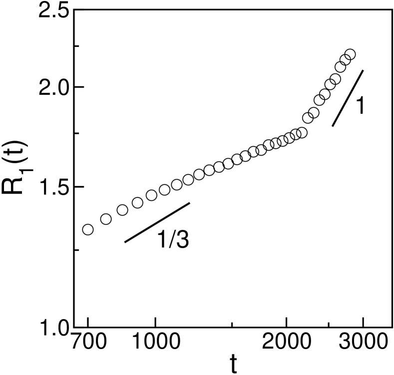
Figure 2: Time-dependence of the wetting-layer thickness [$R_{1}(t)$ vs. $t$] of the SDSD profiles on a log-log scale. The straight lines have slope 1/3 (diffusive regime) and 1 (viscous hydrodynamic regime), respectively.

An important characteristic of the SDSD profiles is the time-dependence of the wetting-layer thickness $R_{1}(t)$. This is defined as the first zero-crossing of the laterally-averaged depth profiles in Fig. 1. In Fig. 2, we plot $R_{1}(t)$ vs. $t$ for the evolution shown in Fig. 1. The growth dynamics is power-law, $R_{1}(t)\sim t^{\theta}$, with $\theta\simeq 1/3$ for $t\lesssim 2000$ and $\theta\simeq 1$ for $t\gtrsim 2000$. For these system sizes, we can go up to $t\simeq 3000$ before encountering finite-size effects due to the lateral domain size becoming an appreciable fraction of the system size $L$.

How can one understand this crossover? At early times, the wetting layer grows by the diffusive transport of $A$ from bulk domains of size $R\sim{(\sigma t)}^{1/3}$ (with chemical potential $\mu\simeq\sigma/R$, $\sigma$ being the surface tension) to the flat surface layer of size $\simeq\infty$ (with $\mu\simeq 0$). If we neglect the very early potential-dependent growth regime [34], we have

$$\frac{dR_{1}}{dt}\simeq\frac{\sigma}{Rh}\simeq\frac{\sigma}{RR_{1}},$$ (3)

where $h\sim R_{1}$ is the thickness of the depletion layer (see Fig. 1). From Eq. (3), we readily obtain the Lifshitz-Slyozov (LS) growth law: $R_{1}\sim{(\sigma t)}^{1/3}$. At later times, bulk tubes establish contact with the wetting layer and material is pumped hydrodynamically to the surface. The subsequent growth is analogous to that in phase separation of fluids – we expect $R_{1}(t)\sim t$ (viscous hydrodynamic regime) which crosses over to $R_{1}(t)\sim t^{2/3}$ (inertial hydrodynamic regime). The latter stage is presently not accessible via MD simulations [25], due to computational limitations. However, our results for wetting-layer dynamics in Fig. 2 appear to access the viscous regime, albeit in a limited time-window. We remark that the crossover time ($t_{c}\simeq 2000$) is consistent with that reported by Ahmad et al. [25] in an MD simulation of bulk phase separation with similar parameter values. Clearly, we need substantially larger system sizes to obtain an extended regime of linear growth in the viscous regime. Notice that the crossover in Fig. 2 is quite sharp, suggesting that there is a rapid pumping of material to the wetting layer when the bulk tubes first make contact.

Second, we present results for the kinetics of SE. In this case, the system size was $L^{2}\times D$ with $L=32,D=64$ ($N=66536$). As the bulk remains homogeneous, the lateral size $L$ (in the $x,y$ directions) is not severely constrained. However, in the direction perpendicular to the surface at $z=0$, we need sufficiently large $D$ to ensure decay of the enrichment profiles as $z\to D$. For the range of times studied here ($t\leq 7000$), test runs with other linear dimensions showed that $D=64$ is large enough to eliminate finite-size effects. In Fig. 3, we show the laterally-averaged profiles and an evolution snapshot (inset) for the kinetics of SE. The quench temperature was $T=2.0\simeq 1.41T_{c}$. The depth profiles were obtained using the same procedure as for SDSD, as an average over $50$ independent runs. The surface potential parameters were $\epsilon_{r}=0.5$ and $\epsilon_{a}=3.0$.

As expected, the morphology for SE is quite different from that in the SDSD case (cf. Fig. 1). There is a thin enrichment layer of $A$ at the surface. Due to the conservation of the order parameter, there must be a corresponding depletion layer which decays to $\psi_{\textrm{av}}\simeq 0$ in the bulk. These profiles are in agreement with the experimental observations of Jones et al. [18] on blends of deuterated and protonated polystyrene, and the experimental results of Mouritsen [35] on biopolymer mixtures. Notice that similar profiles are seen for SDSD if the system is quenched to the metastable region of the phase diagram [34]. The evolution dynamics in that case is analogous to the SE problem, as long as droplets are not nucleated in the system.

For the case with diffusive dynamics, Binder and Frisch [36] and Frisch et al. [37, 38] have studied the morphology of SE profiles in the framework of a linear theory. They find that the SE profiles have a double-exponential form:

$$\psi(z,t)\simeq B_{-}(t)\,\mathrm{e}^{-z/\xi_{-}(t)}-B_{+}(t)\,\mathrm{e}^{-z/\xi_{+}(t)},$$ (4)

with amplitudes $B_{-}(t),B_{+}(t)>0$. The quantities $B_{-}(t)$ and $\xi_{-}(t)$ rapidly saturate to their equilibrium values $a_{1}$ and $b_{1}$, which depend on the surface potential. The other length scale $\xi_{+}(t)$ grows diffusively with time, and $B_{+}(t)$ shows a corresponding decay:

$$B_{+}(t)\simeq a_{2}\,t^{-1/2},\qquad\xi_{+}(t)\simeq b_{2}\,t^{1/2}.$$ (5)

The conservation constraint requires that $B_{-}\xi_{-}=B_{+}\xi_{+}$. In Fig. 3, we see that the double-exponential function in Eq. (4) describes the SE profiles very well.

What about the parameters of the double-exponential profile? As for the diffusive case, we find that $B_{-}$ and $\xi_{-}$ rapidly saturate to their equilibrium values and may be treated as static quantities. The growing length scale is $\xi_{+}(t)$ – we plot $\xi_{+}$ vs. $t$ for different surface field strengths in Fig. 4(a). The early-time dynamics is consistent with diffusive growth ($\xi_{+}\sim t^{1/2}$), but again there is a crossover at $t\sim t_{c}$ to a hydrodynamic regime ($\xi_{+}\sim t$). The crossover is also seen in the thickness of the SE layer. For the profile in Eq. (4), the zero is located at $Z_{0}(t)\simeq\xi_{-}\ln(B_{-}/B_{+})$. Thus, we expect $Z_{0}(t)\sim\ln t$ in both the time-regimes of Fig. 4(a), but the slope should be steeper for $t>t_{c}$. This is precisely the behavior seen in Fig. 4(b), where we plot our MD results for $Z_{0}(t)$ vs. $t$ on a log-linear scale. This confirms that there is a crossover in the growth exponent from the diffusive regime ($\theta\simeq 0.5$) to the hydrodynamic regime ($\theta\simeq 1.0$).

To understand the crossover in Fig. 4, consider the dimensionless evolution equation for the order parameter in the presence of a fluid velocity field $\vec{v}(\vec{r},t)$ [21, 22]:

$$\frac{\partial}{\partial t}\psi(\vec{r},t)=\nabla^{2}\mu-\vec{v}\cdot\vec{\nabla}\psi,$$ (6)

where the chemical potential (for $T>T_{c}$) is $\mu=\psi+\psi^{3}-(1/2)\nabla^{2}\psi$. For the SE problem, the system is homogeneous in the directions parallel to the surface. Thus, we set $\psi(\vec{r},t)\simeq\psi(z,t)$ and $v_{z}(\vec{r},t)\simeq v_{z}(z,t)$. Then, Eq. (6) becomes

$$\frac{\partial}{\partial t}\psi(z,t)=\frac{\partial^{2}\mu}{\partial z^{2}}-v_{z}\frac{\partial\psi}{\partial z}.$$ (7)

We use the functional form of $\psi(z,t)$ in Eq. (4) to estimate the dominant contribution to the various terms in Eq. (7) at $z\sim O(\xi_{+})$, i.e., far from the surface [39]. We have

$$\frac{\partial\psi}{\partial t}\sim\frac{1}{\xi_{+}^{2}}\frac{d\xi_{+}}{dt},\qquad\frac{\partial^{2}\mu}{\partial z^{2}}\sim\frac{1}{\xi_{+}^{3}},\qquad v_{z}\frac{\partial\psi}{\partial z}\sim\frac{v_{z}}{\xi_{+}^{2}}.$$ (8)

For $T>T_{c}$, the bulk is homogeneous and there is no large-scale structure formation in the composition or velocity fields. As the system is incompressible, the velocity field obeys $\vec{\nabla}\cdot\vec{v}=0$ or $\partial v_{z}/\partial z=0$ in the laterally homogeneous case, so that $v_{z}\sim$ constant. Notice that $v_{z}<0$ as there is a net current of the preferred component A towards the enrichment layer. This current is dissipated at the surface by the formation of locally inhomogeneous structures. At early times, the diffusive term in Eq. (7) dominates, yielding $\xi_{+}\sim t^{1/2}$. At late times, the convective term in Eq. (7) is dominant, giving a crossover to $\xi_{+}\sim v_{z}t$. The precise dependence of the crossover time on various physical parameters can be estimated by considering the dimensional version of Eq. (6) in conjunction with the Navier-Stokes equation for the velocity field [21, 22].

In summary, we have presented comprehensive MD results for the kinetics of SDSD and SE in binary mixtures at wetting surfaces. Both the SDSD wetting layer and the SE layer show a crossover from a diffusive regime (with $R_{1}\sim t^{1/3}$ and $\xi_{+}\sim t^{1/2}$) to a hydrodynamic regime (with $R_{1}\sim t$ and $\xi_{+}\sim t$). These crossovers can be understood by simple phenomenological arguments. Our MD results are of great experimental relevance as most studies of these problems are done on polymer or fluid mixtures. We hope that our results in this paper will provoke fresh experimental interest in this problem, and our theoretical results will be subjected to experimental confirmation.

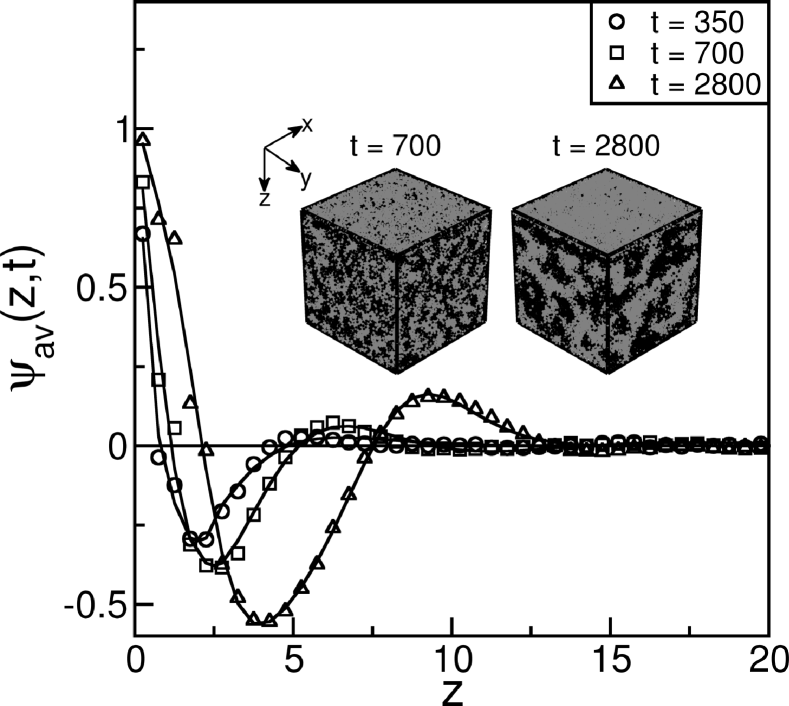
Figure 1: Kinetics of surface-directed spinodal decomposition (SDSD) in a binary ($AB$) Lennard-Jones (LJ) mixture. An impenetrable surface (located at $z=0$) attracts the $A$-particles. The surface field strengths are $\epsilon_{r}=0.5,\epsilon_{a}=0.6$, and the temperature is $T=1.0\simeq 0.7\,T_{c}$. The other simulation details are given in the text. Main figure: Laterally-averaged order parameter profiles [$\psi_{\textrm{av}}(z,t)$ vs. $z$] at $t=350,700,2800$ MD units. Inset: Evolution snapshots at $t=700,2800$. The $A$-particles are marked gray and the $B$-particles are marked black.

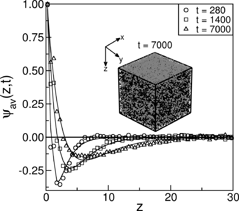
Figure 3: Kinetics of surface enrichment (SE) for an $AB$ mixture in contact with a surface (located at $z=0$) which attracts the $A$-particles. We set $\epsilon_{r}=0.5,\epsilon_{a}=3.0$, and $T=2.0\simeq 1.41\,T_{c}$. The other simulation details are provided in the text. Main figure: Plot of $\psi_{\textrm{av}}(z,t)$ vs. $z$ at $t=280,1400,7000$ MD units. The double-exponential fits for the SE profiles are shown as solid lines. Inset: Evolution snapshot at $t=7000$. The $A$-particles are marked gray and the $B$-particles are marked black.

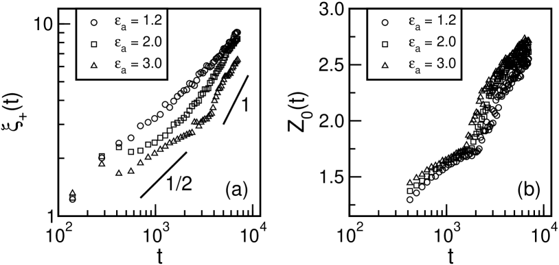
Figure 4: Evolution kinetics of SE profiles. (a) Time-dependence of $\xi_{+}$ on a log-log scale for $\epsilon_{r}=0.5$ and $\epsilon_{a}=1.2,2.0,3.0$. The lines of slope 1/2 and 1 correspond to diffusive and hydrodynamic growth, respectively. (b) Time-dependence of the zero-crossing $Z_{0}(t)$ on a log-linear scale.

References

- [1] R. A. L. Jones, L. J. Norton, E. J. Kramer, F. S. Bates, and P. Wiltzius, Phys. Rev. Lett. 66, 1326 (1991).
- [2] G. Krausch, C.-A. Dai, E. J. Kramer, and F. S. Bates, Phys. Rev. Lett. 71, 3669 (1993).
- [3] J. Liu, X. Wu, W. N. Lennard, and D. Landheer, Phys. Rev. B 80, 041403 (2009).
- [4] C.-H. Wang, P. Chen, and C.-Y. D. Lu, Phys. Rev. E 81, 061501 (2010).
- [5] G. Krausch, Mater. Sci. Eng. Rep. R14, 1 (1995); M. Geoghegan and G. Krausch, Prog. Polym. Sci. 28, 261 (2003).
- [6] S. Puri and H. L. Frisch, J. Phys.: Condens. Matter 9, 2109 (1997).
- [7] S. Puri, J. Phys.: Condens. Matter 17, R101 (2005).
- [8] S. K. Das, S. Puri, J. Horbach, and K. Binder, Phys. Rev. E 72, 061603 (2005); Phys. Rev. E 73, 031604 (2006); Phys. Rev. Lett. 96, 016107 (2006).
- [9] L.-T. Yan and X. M. Xie, J. Chem. Phys. 128, 034901 (2008).
- [10] L.-T. Yan, J. Li, and X. M. Xie, J. Chem. Phys. 128, 224906 (2008).
- [11] K. Binder, S. Puri, S. K. Das, and J. Horbach, J. Stat. Phys. 138, 51 (2010).
- [12] J. W. Cahn, J. Chem. Phys. 66, 3667 (1977).
- [13] M. E. Fisher, J. Stat. Phys. 34, 667 (1984).
- [14] P. G. de Gennes, Rev. Mod. Phys. 57, 827 (1985).
- [15] S. Dietrich, in Phase Transitions and Critical Phenomena, edited by C. Domb and J. L. Lebowitz (Academic Press, London, 1988), Vol. 12, p. 1.
- [16] T. Young, Philos. Trans. R. Soc. London, Ser. A 95, 69 (1805).
- [17] Y. S. Lipatov, in Encyclopedia of Surface and Colloid Science, edited by P. Somasundaran and A. T. Hubbard (Taylor and Francis, New York, 2006).
- [18] R. A. L. Jones, E. J. Kramer, M. H. Rafailovich, J. Sokolov, and S. A. Schwarz, Phys. Rev. Lett. 62, 280 (1989).
- [19] M. Geoghegan, T. Nicolai, J. Penfold, and R. A. L. Jones, Macromolecules 30, 4220 (1997).
- [20] H. Wang, J. F. Douglas, S. K. Satija, R. J. Composto, and C. C. Han, Phys. Rev. E 67, 061801 (2003).
- [21] A. J. Bray, Adv. Phys. 43, 357 (1994).
- [22] Kinetics of Phase Transitions, edited by S. Puri and V.K. Wadhawan (CRC Press, Boca Raton, Florida, 2009).
- [23] V. M. Kendon, M. E. Cates, I. Pagonabarraga, J.-C. Desplat, and P. Bladon, J. Fluid Mech. 440, 147 (2001).
- [24] A. J. Wagner and M. E. Cates, Europhys. Lett. 56, 556 (2001).
- [25] S. Ahmad, S. K. Das, and S. Puri, Phys. Rev. E 82, 040107 (2010).
- [26] S. Bastea, S. Puri, and J. L. Lebowitz, Phys. Rev. E 63, 041513 (2001).
- [27] H. Tanaka, J. Phys.: Condens. Matter 13, 4637 (2001).
- [28] S. K. Das, J. Horbach, and K. Binder, J. Chem. Phys. 119, 1547 (2003).
- [29] S. K. Das, J. Horbach, K. Binder, M. E. Fisher, and J. V. Sengers, J. Chem. Phys. 125, 024506 (2006).
- [30] S. K. Das, M. E. Fisher, J. V. Sengers, J. Horbach, and K. Binder, Phys. Rev. Lett. 97, 025702 (2006).
- [31] M. P. Allen and D. J. Tildesley, Computer Simulation of Liquids (Clarendon Press, Oxford, 1987).
- [32] Monte Carlo and Molecular Dynamics of Condensed Matter Systems, edited by K. Binder and G. Ciccotti (Italian Physical Society, Bologna, 1996).
- [33] S. K. Das and K. Binder, Europhys. Lett. (in press).
- [34] S. Puri and K. Binder, Phys. Rev. Lett. 86, 1797 (2001); Phys. Rev. E 66, 061602 (2002).
- [35] O. G. Mouritsen (private communication).
- [36] K. Binder and H. L. Frisch, Z. Phys. B 84, 403 (1991).
- [37] H. L. Frisch, S. Puri, and P. Nielaba, J. Chem. Phys. 110, 10514 (1999).
- [38] S. Puri and H. L. Frisch, J. Chem. Phys. 79, 5560 (1993).
- [39] P.K. Jaiswal, S. Puri and S.K. Das, J. Chem. Phys. 133, 154901 (2010).