Stochastic Approximation and Modern Model-Based Designs for Dose-Finding Clinical Trials

Abstract

In 1951 Robbins and Monro published the seminal article on stochastic approximation and made a specific reference to its application to the “estimation of a quantal using response, nonresponse data.” Since the 1990s, statistical methodology for dose-finding studies has grown into an active area of research. The dose-finding problem is at its core a percentile estimation problem and is in line with what the Robbins–Monro method sets out to solve. In this light, it is quite surprising that the dose-finding literature has developed rather independently of the older stochastic approximation literature. The fact that stochastic approximation has seldom been used in actual clinical studies stands in stark contrast with its constant application in engineering and finance. In this article, I explore similarities and differences between the dose-finding and the stochastic approximation literatures. This review also sheds light on the present and future relevance of stochastic approximation to dose-finding clinical trials. Such connections will in turn steer dose-finding methodology on a rigorous course and extend its ability to handle increasingly complex clinical situations.

1 Introduction

Dose-finding in phase I clinical trials is typically formulated as estimating a prespecified percentile of a dose-toxicity curve. That is, the objective is to identify a dose $\theta$ such that $\pi(\theta)=p$, or equivalently,

$$\theta=\pi^{-1}(p),$$ (1)

where $\pi(x)$ is the probability of toxicity at dose $x$ and is assumed continuous and increasing in $x$. Percentile estimation, often seen in bioassay, is a well-studied problem for which statisticians have an extensive set of tools; see the books by Finney (1978) and Morgan (1992). There are, however, two practical aspects of clinical studies that distinguish phase I dose-finding from the classical bioassay problem. First, the experimental units are humans. An implication is that the subjects should be treated sequentially with respect to some ethical constraints (e.g., Section 2.3.1). As such, dose-finding is as much a design problem as an analysis problem. Second, the actual doses administered to the subjects are confined to a discrete panel of levels, denoted by $\{d_{1},\ldots,d_{K}\}$, with $\pi(d_{1})<\cdots<\pi(d_{K})$. Therefore, it is possible that $\pi(d_{k})\neq p$ for all $k$, and the working objective then is to identify the dose

$$\nu=\arg\min_{d_{k}}|\pi(d_{k})-p|.$$ (2)

Apparently, the continuous dose-finding objective $\theta$ and the discrete objective $\nu$ are close to each other. However, in this article, we will see that discretized versions of methods developed for $\theta$ are not necessarily good solutions for $\nu$. This special section of Statistical Science also consists of four other articles that review some benchmarks in the recent development of the so-called model-based methods for dose-finding studies. In a nutshell, a model-based method makes dose decisions based on the explicit use of a dose-toxicity model. That is, the toxicity probability at dose $x$, $\pi(x)$, is postulated to be $F(x,\phi_{0})$ for some true parameter value $\phi_{0}$. This is in contrast to the class of algorithm-based designs whereby a set of dose-escalation rules are prespecified for any given dose without regard to the observations at the other doses. Section 2 of this article will present a brief history of the development of the modern dose-finding methods and define the scope of this special issue.

In addition, this article complements the other articles in two ways. First, it consolidates the key theoretical dose-finding criteria that are otherwise scattered in the literature (Section 2.3). Second, it compares and contrasts the dose-finding literature with the large literature on stochastic approximation (Section 3); the former primarily addresses the discrete objective $\nu$, whereas the latter deals with $\theta$. While this literature synthesis is of intellectual interest, it also sheds light on how we may tailor the well-studied stochastic approximation method to meet the practical needs in dose-finding studies (Section 4). Section 5 will end this article with some future directions in dose-finding methodology.

2 Modern Dose-Finding Methods

2.1 A Brief History

This article uses the work of Storer and DeMets (1987) as a historical line to define the modern statistical literature of dose-finding. Little discussion and formal formulation of the dose-finding problem existed in the pre-1987 statistical literature; an exception was the article by Anbar (1984). While dose-finding in cancer trials was discussed as early as in the 1960s in the biomedical communities, a well-defined quantitative objective such as (2) was absent in the communications; see the work of Schneiderman (1965) and Geller (1984), for example. The article by Storer and DeMets (1987) is the earliest reference, to the best of my knowledge, that engages the clinical readership with the idea of percentile estimation. The authors point out the arbitrary estimation properties associated with the traditional 3$+$3 algorithm used in actual dose-finding studies in cancer patients. The 3$+$3 algorithm identifies the so-called maximum tolerated dose (MTD) using the following dose-escalation rules after enrolling every group of three subjects: let $x_{j}$ denote the dose given to the $j$th group of subjects and suppose $x_{j}=d_{k}$; then

$$x_{j+1}=\cases{d_{k+1},&\mbox{if $z_{k}/n_{k}<0.33$,}\cr d_{k},&\mbox{if $z_{k}=1$ and $n_{k}=3$,}\cr d_{k-1},&\mbox{if $z_{k}\geq 2$,}\vspace{-2pt}}$$ (3)

where $n_{k}$ and $z_{k}$ respectively denote the cumulative sample size and number of toxicities at dose $d_{k}$. The trial will be terminated once a de-escalation occurs, and the next lower dose will be called the MTD. In the sequel, Storer (1989) deduced from the 3$+$3 algorithm (3) that a cancer dose-finding study aims to estimate the 33rd percentile (i.e., $p=0.33$). While it has now emerged that the target is likely lower than the 33rd percentile with $p$ being between 0.16 and 0.25, their work has shaped the subsequent development of dose-finding methods in both the statistical and biomedical literatures, and the MTD has since been defined invariably as a dose associated with a prespecified toxicity probability $p$.

O’Quigley, Pepe and Fisher (1990) proposed the continual reassessment method (CRM) in 1990. The CRM is the first model-based method in the modern dose-finding literature. The main idea of the method is to treat the next subject or group of subjects at the dose with toxicity probability estimated to be closest to the target $p$. Precisely, suppose we have observations from the first $j$ groups of subjects and compute the posterior mean $\hat{\phi}_{j}$ of $\phi$ given these observations. Then the next group of subjects will be treated at

$$x_{j+1}=\arg\min_{d_{k}}|F(d_{k},\hat{\phi}_{j})-p|.$$ (4)

A similar idea is adopted in most model-based designs proposed since 1990. One example is the escalation with overdose control (EWOC) by Babb, Rogatko and Zacks (1998), who applied the continual reassessment notion but estimated the MTD with respect to an asymmetric loss function which places heavier penalties on overdosing than underdosing. O’Quigley and Conaway (2010) and Tighiouart and Rogatko (2010) in this special issue review the CRM and the EWOC and their respective extensions. Another CRM-like design is the curve-free method by Gasparini and Eisele (2000) who estimated the dose-toxicity curve using a Bayesian nonparametricmethod in an attempt to avoid bias due to model misspecification. Leung and Wang (2001) proposed an analogous frequentist version that uses isotonic regression for estimation. Other model-based designs include the Bayesian decision-theoretic design(Whitehead and Brunier, 1995), the logistic dose-ranging strategy (Murphy and Hall, 1997), andBayesian $c$-optimal design (Haines, Perevozskaya, and Rosenberger, 2003).

The late 1990s saw an increasing interest in algorithm-based designs. Durham, Flournoy and Rosenberger (1997) proposed a biased coin design by which the dose for the next subject is reduced if the current subject has a toxic outcome, and the dose is escalated with a probability $p/(1-p)$ otherwise. The biased coin design is a randomized version of the Dixon and Mood (1948) up-and-down design. Motivated by its similarity to the traditional design, Cheung (2007) studied a class of stepwise procedures that includes (3) as a special case. Yet another algorithm-based method was proposed by Ji, Li, and Bekele (2007) who made interim decisions based on the posterior toxicity probability interval associated with each dose. The impetus for these algorithm-based designs is simplicity: the decision rules can be charted prior to the trial, so that the clinical investigators know exactly how doses will be assigned based on the observed outcomes.

In order to make dose-finding techniques relevant to clinical practice, statisticians have responded to the realistically complicated clinical situations such as time-to-toxicity endpoints (Cheung and Chappell, 2000) and combination treatments (Thall et al., 2003). While the core dose-finding objective remains a percentile estimation problem, the complexity of dose-finding methods has grown rapidly in the literature, with most innovations taking the model-based approach. Thall (2010) in this special issue will review the major development of these complex designs.

Most (model-based) designs in the literature up to this point take the myopic approach by which the dose assignment is optimized with respect to the next immediate subject without regard to the future subjects. Bartroff and Lai (2010) in this issue break away from this direction and propose a model-based method from an adaptive control perspective. While this work attempts to solve a specific Bayesian optimization problem, it also sets a new direction in the modern dose-finding techniques; see Section 3 of this article.

2.2 Why Model-Based Now

A model-based design allows borrowing strength from information across doses. This characteristic appeals to statisticians and clinicians alike, especially because of the typically small-to-moderate sample sizes seen in early-phase clinical studies. As clinicians begin to appreciate the crucial role of dose-finding in the entire drug development program and the value of statistical inputs to reconcile the ethical and research aspects in early-phase trials, their discussions have revolved around model-based innovations such as the CRM (Ratain et al., 1993) and the EWOC (Eisenhauer et al., 2000). The increasing number of applications in actual trials (Muller et al., 2004) indicates the clinical awareness and readiness for these model-based methods.

When compared to the simplicity of algorithm-based methods, the model-based approaches are computationally complex and require special programming before and during the implementation of a trial. Thanks to the advances of computing algorithms (e.g., Markov chain Monte Carlo) and computer technology, however, trial planning with extensive simulation has become feasible. This being the case, a full-scale dynamic programming can still stretch the computing resource; see the article by Bartroff and Lai (2010) for some comparison of computational times. In addition, statistician-friendly software has become increasingly available for the planning and execution of these model-based designs, for example, the dfcrm package in R (Cheung, 2008). These indicators of computational maturity transform the model-based designs into practical tools for dose-finding trials.

Finally, the development of dose-finding theory and dose-response models in the past two decades lends scientific rigor to the complexity of the model-based methods. Indeed, the goal of this special issue is to review the theoretical and modeling progress made in the modern dose-finding literature, andthereby demonstrate the full promise, and perhaps challenges, of the model-based methods.

2.3 Some Theoretical Criteria

In a typical dose-finding trial, subjects are enrolled in small groups of size $m\geq 1$. The enrollment plan is said to be fully sequential when $m=1$. Let $x_{i}$ denote the dose given to the $i$th group of subject(s). Thus, the sequence $\{x_{i}\}$ forms the design of a dose-finding study. As most dose-finding methods are outcome-adaptive, each design point $x_{i}$ is random and depends on the previous observation history. Evaluation of a dose-finding method therefore involves the study of its design space with respect to some ethical and estimation criteria. This section will review some key dose-finding criteria including coherence, rigidity, indifference intervals, and unbiasedness.

2.3.1 Coherence

First, consider fully sequential trials with $m=1$, so that each human subject is an experimental unit. An ethical principle, coined coherence by Cheung (2005), dictates that no escalation should take place for the next enrolled subject if the current subject experiences some toxicity, and that dose reduction for the next subject is not appropriate if the current subject has no sign of toxicity. Precisely, let $Y_{i}$ denote the toxicity outcome of the $i$th subject. An escalation for the subject is said to be coherent only when $Y_{i-1}=0$; likewise, a de-escalation is coherent only when $Y_{i-1}=1$. Extending the notion of coherence for each move, one can naturally define coherence as a property of a dose-finding method:

Property 1 ((Coherence)).

A dose-finding design $\mathcal{D}$ is said to be coherent in escalation if with probability 1

$$P_{\mathcal{D}}(U_{i}>0|Y_{i-1}=1)=0$$ (5)

for all $i$, where $U_{i}=x_{i}-x_{i-1}$ is the dose increment from subject $i-1$ to $i$, and $P_{\mathcal{D}}(\cdot)$ denotes probability computed under the design $\mathcal{D}$. Analogously, the design is said to be coherent in de-escalation if with probability 1

$$P_{\mathcal{D}}(U_{i}<0|Y_{i-1}=0)=0$$ (6)

for all $i$.

It is important to note that coherence is motivated by ethical concerns, and hence may not correspond to efficient estimation of the dose-toxicity curve. For example, in bioassay, an efficient design obtained by sequentially maximizing some function of the information may induce incoherent moves, and thus is not appropriate for human trials; see the work of McLeish and Tosh (1990), for example.

An algorithm-based design can explicitly incorporate dose decision rules that respect the coherence principles; see the biased coin design. For a model-based design, on the other hand, it is not immediately clear whether coherence necessarily holds. There are three general ways to ensure coherence in practice. First, one could adopt model-based methods that have been proven coherent analytically. This includes the one-stage Bayesian CRM. Second, one could take a numerical approach. Let $N$ denote the sample size of a trial. Then the design space is completely generated by the first $N-1$ binary toxicity observations, and thus consists of $2^{N-1}$ possible design outcomes. Therefore, one could establish coherence (for a given $N$) by enumerating all possible outcomes and verifying that there is no incoherent move. In some cases, the number of outcomes can be immensely reduced to the order of $N$; see Theorem 1 in the article by Cheung (2005). Third, one could enforce coherence by restriction when the model-based dose assignment is incoherent. Applying coherence restrictions is common in practice (Faries, 1994) and is the most straightforward approach for complex designs. On the other hand, the restricted moves need to be examined carefully lest they should cause an incompatibility problem as defined by Cheung (2005).

In practice, the enrollment plan is often small-group sequential, that is, $m>1$, in order to reduce the number of interim decisions and hence trial duration. In this case, each group of subjects may be viewed as an experimental unit. A generalized version of Property 1 can be stated as:

Property 1^′ ((Group coherence)).

A dose-finding design $\mathcal{D}$ is said to be group coherent in escalation if with probability 1

$$P_{\mathcal{D}}(U_{i}>0|\bar{Y}_{i-1}\geq p)=0$$ (7)

for all $i$, where $U_{i}=x_{i}-x_{i-1}$ now denotes the dose increment from group $i-1$ to $i$ and $\bar{Y}_{i-1}$ is the observed proportion of toxicities in group $i-1$. Analogously, the design is said to be group coherent in de-escalation if with probability 1

$$P_{\mathcal{D}}(U_{i}<0|\bar{Y}_{i-1}\leq p)=0$$ (8)

for all $i$.

It is easy to see that (7) and (8) reduce to (5) and (6), respectively, when $m=1$ for $p\in(0,1)$.

2.3.2 Rigidity and sensitivity

A design sequence $\{x_{n}\}$ is strongly consistent for $\theta$ if $x_{n}\rightarrow\theta$ with probability 1. For trials allowing only a discrete number of test doses as in (2), consistency means $x_{n}=\nu$ eventually with probability 1. Consistency, a desirable statistical property in general, has an ethical connotation in dose-finding studies because it implies all subjects enrolled after a certain time point will be treated at $\nu$, which is the desired dose.

Property 2 ((Rigidity)).

A dose-finding design $\mathcal{D}$ is said to be rigid if for every $0<p_{L}<\pi(\nu)<p_{U}<1$ and all $n\geq 1$,

$$P_{\mathcal{D}}\{x_{n}\in\mathcal{I}_{\pi}(p_{L},p_{U})\}<1,$$

where $\mathcal{I}_{\pi}(p_{L},p_{U})=\{x\dvtx p_{L}\leq\pi(x)\leq p_{U}\}$.

It is easy to see that consistency excludes the rigidity problem. In other words, Property 2 implies that a design is inconsistent. In particular, rigidity occurs when a CRM-like procedure is applied in conjunction with nonparametric estimation. Hence, such a nonparametric design is inconsistent. This is quite interesting and somewhat counterintuitive, because nonparametric estimation is introduced with an intention to remove bias and to enhance theprospect of consistency.

To illustrate, consider a design that starts at dose level 1, enrolls subjects in groups of size $m=2$, and assigns the next group at $\arg\min_{k}|\tilde{p}_{k}-p|$ where $\tilde{p}_{k}$ is an estimate of $\pi(d_{k})$ based on isotonic regression, and the target is $p=0.20$. Now suppose that none of the subjects in the first group has a toxic outcome. Then suppose the second group enters the trial at dose level 2, with one of the two experiencing toxicity. Based on these observations, the isotonic estimates are $\tilde{p}_{1}=0.00$ and $\tilde{p}_{2}=0.50$, which bring the trial back to dose level 1. From this point on, because there is no parametric extrapolation to affect the estimation of $\pi(d_{2})$ by the data collected at $d_{1}$, the isotonic estimate $\tilde{p}_{2}$ will be no smaller than 0.50 regardless of what happens at $d_{1}$, that is, $|\tilde{p}_{2}-0.20|\geq 0.30$. As a result, $|\tilde{p}_{1}-0.20|<0.30\leq|\tilde{p}_{2}-0.20|$ if $\tilde{p}_{1}\leq 0.20$. That is, the trial will stay at dose level 1 even if there is a long string of nontoxic outcomes there!

This example demonstrates that nonparametric estimation and the sequential sampling plan together cause rigidity through an “extreme” overestimate of $\pi(d_{2})$ based on small sample size. The probability of this extreme overestimation is nonnegligible indeed: if dose level 2 is the true MTD with $\pi(d_{2})=0.20$, then the probability that the trial is confined to the suboptimal dose 1 is at least 0.36 by a simple binomial calculation. Cheung (2002) constructed a similar numerical example for the Bayesian nonparametric curve-free method, and suggested that the rigidity probability can be reduced by using an informative prior to add smoothness to the estimation.

Due to ethical constraints such as coherence and the discrete design space, it may be challenging to achieve consistency without strong model assumptions. For example, the CRM has been shown to be consistent under certain model misspecifications, but is not generally so (Shen and O’Quigley, 1996). In this context, Cheung and Chappell (2002) introduced the indifference interval as a sensitivity measure of how close a design may approach $\nu$ on the probability scale:

Property 3 ((Indifference interval)).

The indifference interval of a dose-finding design $\mathcal{D}$ exists and is equal to $p\pm\delta$ if there exist $N>0$ and $\delta\in(0,p)$ such that

$$P_{\mathcal{D}}\{x_{n}\in\mathcal{I}_{\pi}(p-\delta,p+\delta)\mbox{ for all $n\geq N$}\}=1.$$

Apparently, the smaller the half-width $\delta$ of a design’s indifference interval is, the closer the design converges to the MTD; whereas a large $\delta$ indicates the design is sensitive to the underlying $\pi$. The sensitivity of the design $\mathcal{D}$ can thus be measured by $\delta$. Specifically, a design with half-width $\delta$ (for some $\delta<p$) will be called a $\delta$-sensitive design.

It is clear that if a design $\mathcal{D}$ is consistent for $\nu$, then it is $\delta$-sensitive; that is, one may choose $\delta$ so that $\pi(\nu)\in p\pm\delta$. Also, if $\mathcal{D}$ is $\delta$-sensitive, then it is nonrigid. Thus, while consistency appears to be too difficult and nonrigidity too nondiscriminatory for a dose-finding design, $\delta$-sensitivity seems to be a reasonable design property. Cheung and Chappell (2002) prescribed a way to calculate the indifference interval of the CRM, that is, the CRM is $\delta$-sensitive. Moreover, Lee and Cheung (2009) showed that the CRM can be calibrated to achieve any $\delta$ level of sensitivity. However, it should be noted that indifference interval is an asymptotic criterion. As such, a small $\delta$ does not necessarily yield good finite-sample properties.

2.3.3 Unbiasedness

The performance of a reasonable dose-finding design is expected to improve as the underlying dose-toxicity curve $\pi$ becomes steep. This property, called unbiasedness by Cheung (2007), is formulated as follows:

Property 4 ((Unbiasedness)).

Let $p_{i}=\pi(d_{i})$ denote the true toxicity probability at dose $d_{i}$. A design $\mathcal{D}$ is said to be unbiased if [(a)]

$P_{\mathcal{D}}(x_{n}=d_{k})$ is nonincreasing in $p_{i^{\prime}}$ for $i^{\prime}\leq k$, and

$P_{\mathcal{D}}(x_{n}=d_{k})$ is nondecreasing in $p_{i}$ for $i>k$.

For the special case with $d_{k}=\nu$ and $\pi(\nu)=p$, unbiasedness implies that the probability of correctly selecting $\nu$ increases as the doses above the MTD become more toxic (i.e., $p_{i}\gg p$), or the doses below less toxic (i.e., $p_{i^{\prime}}\ll p$). In other words, the design will select the true MTD more often as it becomes more separated from its neighboring doses in terms of toxicity probability. A design that satisfies this special case is called weakly unbiased.

One may argue that $\delta$-sensitive designs (e.g., the CRM) are asymptotically weakly unbiased, in that they will be consistent if the underlying dose-toxicity curve $\pi$ becomes sufficiently steep around the MTD; see Figure 1 for an illustration. Unbiasedness has been established only for few designs in the dose-finding literature; an example is the class of stepwise procedures (Cheung, 2007). In practice, extensive simulations are usually required, and are often adequate, to confirm that a design is (weakly) unbiased.

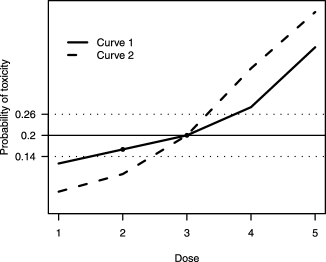
Figure 1: Two dose-toxicity curves under which dose 3 is the MTD with $p=0.20$. A $\delta$-sensitive design with $\delta=0.06$ will eventually select doses 2 or 3 under the shallow curve (curve 1), but will be consistent for dose 3 under the steep curve (curve 2). The horizontal dotted lines indicate the indifference interval.

3 Stochastic Approximation

3.1 The Robbins–Monro (1951) Procedure

Robbins and Monro (1951) introduced the first formal stochastic approximation procedure for the problem of finding the root of a regression function. Precisely, let $M(x)$ be the mean of an outcome variable $Y=Y(x)$ at level $x$, and suppose $M(x)=\alpha$ has a unique root $\theta$ and $\sup_{x}E\{Y^{2}(x)\}<\infty$. Then the stochastic approximation recursion approaches $\theta$ sequentially:

$$x_{i+1}=x_{i}-\frac{1}{ib}(Y_{i}-\alpha)$$ (9)

for some constant $b>0$. It is well established that $x_{n}\rightarrow\theta$ with probability 1. If in addition, the constant $b$ is chosen properly namely $b<2M^{\prime}(\theta)\equiv 2\beta$, then $n^{1/2}(x_{n}-\theta)$ will converge in distribution to a normal variable with mean 0 and variance $\sigma^{2}\{b(2\beta-b)\}^{-1}$ where $\sigma^{2}=\lim_{x\rightarrow\theta}\operatorname{var}\{Y(x)\}$; see the works of Sacks (1958) and Wasan (1969).

It is immediately clear that (9) is applicable to address objective (1) in a clinical trial setting with $M=\pi$ and $\alpha=p$. For one thing, the recursion output is coherent (Property 1) thus passing the first ethical litmus test. It is also easy to see that a small-group sequential version of (9), that is, replace $Y_{i}$ with $\bar{Y}_{i}$, is group coherent (Property 1^′). There are, however, several practical considerations.

The choice of $b$ is crucial. In view of efficiency, the asymptotic variance is minimized when we set $b=\beta$, which is typically unknown in most applications. This leads to the idea of adaptive stochastic approximation where $b$ is replaced by a sequence $b_{i}$ that is strongly consistent for $\beta$ (Lai and Robbins, 1979). However, when the sample size is small-to-moderate, the numerical instability induced by the adaptive choice $b_{i}$ may offset its asymptotic advantage. In this article, for a reason described in Section 4.2, we assume that a good choice of $b$ is available.

The next practical issue is that (9) entails the availability of a continuum of doses. This is seldom feasible in practice. In drug trials, dose availability is often limited by the dosage of a tablet. For treatments involving combination of drugs administered multiple times over a fixed period, each subsequent dose may involve increasing doses and/or frequency of different drugs. For example, Table 1 describes the dose schedules of bortezomib used in a dose-finding trial in patients with lymphoma (Leonard et al., 2005). The first three levels prescribe bortezomib at a fixed dose 0.7 mg/m² with increasing frequency, whereas the next two increments apply the same frequency with increasing bortezomib doses. While we are certain that the risk for toxicity increases over each level, there is no natural scale of dosage (e.g., mg/m²). Thus, assuming that the toxicity probability $\pi(x)$ is well defined on a continuous range of $x$ is artificial.

Table 1: Dose schedules of bortezomib used in Leonard et al. (2005)

Level	Dose and schedule within cycle
1	0.7 mg/m2 on day 1 of each cycle
2	0.7 mg/m2 on days 1 and 8 of each cycle
3	0.7 mg/m2 on days 1 and 4 of each cycle
4	1.0 mg/m2 on days 1 and 4 of each cycle
5	1.3 mg/m2 on days 1 and 4 of each cycle

To tailor the stochastic approximation for the discrete objective $\nu$, an obvious approach is to round the output of (9) to its closest dose at each iteration. For example, suppose that the dose labels are $\{1,\ldots,K\}$, that is, $d_{k}=k$. Then a discretized stochastic approximation may be expressed as

$$x_{i+1}=C\biggl{\{}x_{i}-\frac{1}{ib}(\bar{Y}_{i}-p)\biggr{\}},$$ (10)

where $C(x)$ is the rounded value of $x$ if $0.5\leq x<K+0.5$, and is set equal to 1 and $K$ respectively if $x<0.5$ or $>K+0.5$. Unfortunately, the discretized stochastic approximation is rigid (Property 2). To illustrate, consider applying (10) with $b=0.2$ and a target $p=0.20$ in a trial with $x_{1}=1$ and $m=2$. Then no toxicity event in the first group, that is, $\bar{Y}_{1}=0$, gives $x_{2}=2$. Further suppose that the second group has a 50% toxicity rate ($\bar{Y}_{2}=0.5$). This will bring the trial back to $x_{3}=C(2-0.75)=1$; it is easy to see that the remaining subjects will receive dose 1. To see how rigidity occurs for a general variable type, we observe that since $x_{i}$ is an integer, the update $x_{i+1}$ according to (10) will stay the same as $x_{i}$ if $|(ib)^{-1}(\bar{Y}_{i}-p)|<0.5$, whose probability approaches 1 at a rate of $O(i^{-2})$ according to Chebyshev’s inequality if $Y_{i}$ has a finite variance. If $Y_{i}$ is bounded (e.g., binary), the term $C\{(ib)^{-1}(\bar{Y}_{i}-p)\}$ will always be zero as $i$ becomes sufficiently large, and will not contribute to future updates. This problem, called discrete barrier, is thus built by rounding and the fact that the design points take on a discrete set of levels. In the context of the CRM, Shen and O’Quigley (1996) pointed out similar difficulties in establishing the theoretical properties of dose-finding methods due to the discrete barrier. This is where the modern dose-finding literature departs from the elegant stochastic approximation approach.

3.2 Stochastic Approximation and Model-Based Methods

The Robbins–Monro stochastic approximation is a nonparametric procedure in that the convergence results depend only very weakly on the true underlying $M(x)$. For the case of normal $Y$, interestingly, Lai and Robbins (1979) showed that the recursion output in (9) is identical to the solution $\tilde{x}_{i+1}$ of

$$\sum_{j=1}^{i}Y_{j}-\{\alpha+b(\tilde{x}_{j}-\tilde{x}_{i+1})\}=0$$ (11)

which amounts to maximum likelihood estimation of $\theta$ under a simple linear regression model. This connection between the stochastic approximation and a model-based approach motivates the study of the maximum likelihood recursion in the work of Wu (1985), Wu (1986), and Ying and Wu (1997) for data arising from the exponential family. In particular, for binary $Y$, Wu (1985) proposed the logit-MLE that uses the logistic working model

$$F(x,\theta)=\frac{p\exp\{\tilde{b}(x-\theta)\}}{1-p+p\exp\{\tilde{b}(x-\theta)\}}$$

(12)

$$\eqntext{\mbox{for some $\tilde{b}>0$}}\vspace*{6pt}$$ (13)

and replaces the estimating equation (11) with$\sum_{j=1}^{i}\{Y_{j}-F(\tilde{x}_{j},\tilde{x}_{i+1})\}=0$. Here, we focus on the nonadaptive version, that is, where $\tilde{b}$ is a fixed constant. A maximum likelihood version of the CRM (4) would clearly yield the same design point as $\tilde{x}_{i+1}$ if the design space was continuous. In this regard, the likelihood CRM is an analogue of the logit-MLE for the discrete objective $\nu$.

In order to establish the asymptotic distribution of the logit-MLE (and the maximum likelihood recursion in general), Ying and Wu (1997) showed that the sequence $\tilde{x}_{i+1}$ is asymptotically equivalent to an adaptive Robbins–Monro recursion; see the proof of Theorem 3 in the article by Ying and Wu (1997). While the justification of the model-based logit-MLE relies on its asymptotic equivalence to the nonparametric Robbins–Monro procedure, Wu (1985) showed by simulation that the former is superior to the latter in finite-sample settings with binary data. Similarly, O’Quigley and Chevret (1991) demonstrated that the CRM performs better than the discretized stochastic approximation (10) for the objective $\nu$.

These observations regarding the stochastic approximation, the logit-MLE, and the CRM bear two practical suggestions. First, in typical dose-finding trial settings with binary data and small sample sizes, a model-based approach seems to retain some information that is otherwise lost when using nonparametric procedures. This speculation is madewithout assuming much confidence about the working model. Second, one may study the theoretical (asymptotic) properties of the modern model-based method (e.g., CRM) by tapping the rich stochastic approximation literature, thus giving guidance on the choice of design parameters such as $\tilde{b}$ in (3.2). This can be achieved, of course, only if we can resolve the discrete barrier—we will return to this in Section 4.2.

3.3 Stochastic Approximation and Adaptive Control

Maximum likelihood recursion attempts to optimize the prospect for the next subject by setting the next design point at the current estimate of $\theta$, and is myopic in that it does not consider the dose assignments of future subjects. The Robbins–Monro procedure is therefore myopic by (asymptotic) equivalence. Lai and Robbins (1979) studied the adaptive cost control aspect of the stochastic approximation for normal $Y$ where $C_{n}=\sum_{i=1}^{n}(x_{i}-\theta)^{2}$ is defined as the cost of a design sequence $\{x_{i}\}$ at stage $n$. Specifically, they showed that the cost of (9) is of the order $\sigma^{2}\log n$ if $b<2\beta$. Under some simple linear regression models, Han, Lai, and Spivakovsky (2006) showed that the myopic Bayesian rule is optimal when the slope parameter is known. This suggests that the myopic Robbins–Monro method may also have good adaptive control properties.

The control aspect of the stochastic approximation is less clear for binary data. Bartroff and Lai (2010) addressed the control problem by using techniques in approximate dynamic programming to minimize some well-defined global risk, such as the expectation of the design cost $C_{n}$. The authors demonstrated reduction of the global risk by nonmyopic approaches when compared to the myopic ones including the stochastic approximation and the logit-MLE. The scope of the simulations, however, is confined to situations where the logistic model correctly specifies $\pi$. In addition, their approach is intended for the continuous objective $\theta$, instead of $\nu$.

Further research on the use of nonmyopicapproaches in dose-finding is warranted, especially for practical situations with a discrete set of test doses. The design cost at stage $n$ for the discrete objective $\nu$ can be analogously defined as $C_{n}^{\prime}=\break\sum_{i=1}^{n}(x_{i}-\nu)^{2}$. Then a dose-finding design $\mathcal{D}$ is consistent if and only if $\lim_{n\rightarrow\infty}C_{n}^{\prime}$ is finite almost everywhere. As mentioned earlier, the myopic CRM is not necessarily consistent (as it tries to treat each subject at the current “best” dose). By contrast, designs that spread out the design points (e.g., the biased coin design) allow consistent estimation of $\nu$ at the expense of the enrolled subjects. Neither guarantees a finite $\lim_{n}C_{n}^{\prime}$. An optimal $\mathcal{D}$ for the infinite-horizon control of $C_{n}^{\prime}$ thus seems to resolve the inherent tension between the welfare of enrolled subjects (i.e., the cost is kept low) and the estimation of $\nu$ (i.e., $x_{n}$ is consistent).

4 Ongoing Relevance

4.1 Binary Versus Dichotomized Data

As mentioned earlier, with a binary outcome and small samples, the Robbins–Monro procedure is generally less efficient than model-based methods, and hence may not be suitable for clinical dose-finding where the study endpoint is classified as toxic and nontoxic. In many situations, however, the binary toxic outcome $T$ is defined by dichotomizing an observable biomarker expression $Y$, namely, $T=\mathbf{1}(Y>t_{0})$ for some fixed safety threshold $t_{0}$, where $\mathbf{1}(E)$ denotes the indicator of the event $E$. The biomarker $Y$ apparently contains more information than the dichotomized $T$, and may be used to achieve the dose-finding objective (1) with greater efficiency.

To illustrate, consider the regression model

$$Y=M(x)+\sigma(x)\epsilon,$$ (14)

where $\epsilon$ has a known distribution $G$ with mean 0 and variance 1. Under (14), the toxicity probability can be expressed as $\pi(x)=1-G[\{t_{0}-M(x)\}/\sigma(x)]$ and the continuous dose-finding objective (1) can be shown to be equivalent to the solution to

$$f(x)\equiv M(x)+z_{p}\sigma(x)=t_{0},$$ (15)

where $z_{p}$ is the upper $p$th percentile of $G$. To focus on the comparison between the use of $Y$ and $T$, suppose for the moment that a continuum of dose $x$ is available. Further suppose that a trial enrolls patients in small groups of size $m$. Let $x_{i}$ denote the dose given to the $i$th group, and $Y_{ij}$ the biomarker expression of the $j$th subject in the group. With this experimental setup, we note that

$$O_{i}=\bar{Y}_{i}+[E\{S_{i}/\sigma(x_{i})\}]^{-1}z_{p}S_{i}$$ (16)

is an unbiased realization of $f(x_{i})$, where $S_{i}$ is the sample standard deviation of the observations ingroup $i$. The expectation in (16) can be computed for any given $G$, because $S_{i}/\sigma(x_{i})$ depends on the error variable $\epsilon$ but not $M$ and $\sigma$ under model (14). In other words, $O_{i}$ is observable and is a continuous variable that can be used to generate a stochastic approximation recursion

$$x_{i+1}=x_{i}-(ib)^{-1}(O_{i}-t_{0}).$$ (17)

The design $\{x_{n}\}$ generated by (17) is consistent for $\theta$ under the condition that $\theta$ is the unique solution to (15). This condition holds, for example, when $M$ is strictly increasing and $\sigma$ is nondecreasing in $x$. This is a reasonable assumption for many biological measurements, for which the variability typically increases with the mean. Furthermore, if $b<2\beta$, where $\beta=f^{\prime}(\theta)$ here, then the asymptotic variance of $x_{n}$ is $v_{O}=\lim_{x\rightarrow\theta}\operatorname{var}(O_{i})\{b(2\beta-b)\}^{-1}$. In particular, when $\epsilon$ is standard normal,

$$v_{O}=\frac{\sigma^{2}(\theta)\{1+mz_{p}^{2}(\lambda_{m}-1)\}}{mb(2\beta-b)},$$

where

$$\lambda_{m}=\frac{(m-1)\Gamma^{2}\{(m-1)/2\}}{2\Gamma^{2}(m/2)}.$$

Now, instead of using the recursion (17), suppose that we apply the logit-MLE based on thedichotomized outcomes by solving $\sum_{j=1}^{i}\{\bar{T}_{j}-\break F(\tilde{x}_{j},\tilde{x}_{i+1})\}=0$ where $F$ is defined in (3.2). Then using the results in the article of Ying and Wu (1997), we can show that $\sqrt{n}(\tilde{x}_{n}-\theta)$ converges in distribution to a mean zero normal with variance $v_{T}=p(1-p)\{m\tilde{b}(2\tilde{\beta}-\tilde{b})\}^{-1}$ where $\tilde{\beta}\equiv\pi^{\prime}(\theta)=\beta G^{\prime}(z_{p})/\sigma(\theta)$.

The asymptotic variances of $v_{O}$ and $v_{T}$ are minimized when $b=\beta$ and $\tilde{b}=\tilde{\beta}$, respectively. Thus, the optimal choice depends on unknown parameters. For the purpose of comparing efficiencies, suppose we could set $b$ and $\tilde{b}$ to their respective optimal values. Then the variance ratio is equal to

$$\frac{v_{T}}{v_{O}}=\frac{p(1-p)}{\{G^{\prime}(z_{p})\}^{2}\{1+mz_{p}^{2}(\lambda_{m}-1)\}}$$ (18)

for normal noise, and also represents the asymptotic efficiency of $x_{n}$ relative to $\tilde{x}_{n}$. For $m=3$, the ratio (18) attains a minimum of 1.238 when $p=0.12$ or 0.88. As shown in Figure 2, the efficiency gain can be substantial for any group sizes larger than 2, especially when the target $p$ is extreme.

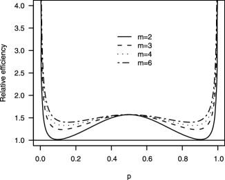
Figure 2: Asymptotic efficiency of $x_{n}$ based on recursion (17) relative to the logit-MLE $\tilde{x}_{n}$.

4.2 Virtual Observations

A particular obstacle to the use of stochastic approximation is the discrete design space used in clinical studies, which creates the discrete barrier (Section 3.1). To overcome the discrete barrier, Cheung and Elkind (2010) introduced the notion of virtual observations. Precisely, the virtual observation of the $i$th group of subjects is defined as

$$V_{i}=O_{i}+b(x_{i}^{*}-x_{i}),$$ (19)

where $x_{i}^{*}$ denotes the assigned dose of the group which can take values on a continuous conceptual scale that represents an ordering of doses. In the situations where the actual given dose $x_{i}$ can take on any real value, we have $x_{i}^{*}\equiv x_{i}$ and $V_{i}\equiv O_{i}$, and thus, the recursion (17) may be used to approach the target dose $\theta$. When $x_{i}$ is confined to $\{1,\ldots,K\}$, Cheung and Elkind (2010) proposed generating a stochastic approximation recursion based on the virtual observations:

$$x_{i+1}^{*}=x_{i}^{*}-\frac{1}{ib}(V_{i}-t_{0}),$$ (20)

and treating the next group of subjects at $x_{i+1}=C(x_{i+1}^{*})$. To initiate the virtual observation recursion, one may set $x_{1}^{*}=x_{1}\in\{1,\ldots,K\}$.

Cheung and Elkind (2010) proved, under mild conditions, that $x_{i+1}^{*}$ generated by (20) is consistent (hence nonrigid) for $\theta_{b}$ for some $\theta_{b}=\nu\pm 0.5$, and hence $x_{i+1}$ for $\nu$. Briefly, for any given $b$, consistency will occur if the neighboring doses of the MTD are sufficiently apart from the MTD in terms of toxicity probability. This is in essence asymptotically weakly unbiased as defined in Section 2.3.3, and can be easily derived from Propositions 2 and 3 of Cheung and Elkind (2010).

With the use of continuous $V$’s, the notion of coherence needs to be re-examined. In particular, the virtual observation recursion (20) will de-escalate if the biomarker expression of the current subjects has a high average ($\bar{Y}_{i}$) or a large variability ($S_{i}$). This is a sensible dose-escalation principle for situations where the variability increases proportionally to the mean.

The idea of virtual observation is to create an objective function

$$h(x)=E(V_{i}|x_{i}^{*}=x)=f\{C(x)\}+b\{x-C(x)\}$$

that is defined on the real line, and has a local slope at $\{1,\ldots,K\}$, such that the solution $\theta$ of (15) can be approximated by the solution $\theta_{b}$ of $h(x)=t_{0}$. Quite importantly, since now the objective function $h$ has a known slope $b$ around $\theta_{b}$ (under some Lipschitz-type regularity conditions), we can use the same $b$ in the recursion (20) as in the definition of virtual observations (19). This design feature enables us to achieve optimal asymptotic variance without resorting to adaptive estimation of the slope of the objective function. It is particularly relevant to early phase dose-finding studies where adaptive stochastic approximation can be unstable due to small sample sizes.

5 Looking to the Future

Statistical methodology for dose-finding trials is by its nature an application-oriented discipline. Consequently, much of the emphasis in the dose-finding literature has been on empirical properties via simulation. However, as the (model-based) methods become increasingly complicated, it is imperative to check their properties against some theoretical criteria so as to avoid pathological behaviors that may not be detected in aggregate via simulations; rather, pathologies such as incoherence and rigidity are pointwise properties that can be found by careful analytical study. As a case in point, the virtual observation recursion (20) is presented in light of the properties described in Section 2.3. Granted, as the data content becomes richer, these theoretical criteria have to be re-examined. Cheung (2010), in another instance, extended the notion of coherence for bivariate dose-finding in the context of phase I/II trials—see the article by Thall (2010) for a review of the bivariate dose-finding objective—and showed how coherence can be used to simplify dose decisions in the complex “black-box” approach of the bivariate model-based methods, and to provide clinically sensible rules.

The idea of virtual observation bridges the stochastic approximation and the modern (model-based) dose-finding literatures. As the Robbins–Monromethod has motivated a large number of extensions and refinements for a wide variety of root-finding objectives, there exists a reservoir of ideas from which we can borrow and apply to dose-finding methods for specialized clinical situations. To name a few, consult the works of Kiefer and Wolfowitz (1952) for finding the maximum of a regression function, and Blum (1954) for multivariate contour-finding. While studying the analytical properties of model-based designs in these specialized situations can be difficult, connection to the theory-rich stochastic approximation procedures allows us to do so with relative ease and elegance, as is the case for the virtual observation recursion (20). In this light, extending the idea of virtual observations for data types other than continuous and multivariate data appears to be a promising “crosswalk” that warrants further research.

References

- Anbar (1984) Anbar, D. (1984). Stochastic approximation methods and their use in bioassay and phase I clinical trials. Commun. Statist. 13 2451–2467.
- Babb, Rogatko and Zacks (1998) Babb, J., Rogatko, A. and Zacks, S. (1998). Cancer phase I clinical trials: Efficient dose escalation with overdose control. Statist. Med. 17 1103–1120.
- Bartroff and Lai (2010) Bartroff, J. and Lai, T. L. (2010). Approximate dynamic programming and its applications to the design of phase I cancer trials. Statist. Sci. 25 245–257.
- Blum (1954) Blum, J. R. (1954). Multidimensional stochastic approximation methods. Ann. Math. Statist. 25 737–744. \MR0065092
- Cheung (2002) Cheung, Y. K. (2002). On the use of nonparametric curves in phase I trials with low toxicity tolerance. Biometrics 58 237–240. \MR1891385
- Cheung (2005) Cheung, Y. K. (2005). Coherence principles in dose-finding studies. Biometrika 92 863–873. \MR2234191
- Cheung (2007) Cheung, Y. K. (2007). Sequential implementation of stepwise procedures for identifying the maximum tolerated dose. J. Amer. Statist. Assoc. 102 1448–1461. \MR2446206
- Cheung (2008) Cheung, Y. K. (2008). Dose-finding by the continual reassessment method (dfcrm). R package version 0.1-2. Available at http://www.r-project.org.
- Cheung (2010) Cheung, Y. K. (2010). Dose Finding by the Continual Reassessment Method. Chapman and Hall, New York. To appear.
- Cheung and Chappell (2000) Cheung, Y. K. and Chappell, R. (2000). Sequential designs for phase I clinical trials with late-onset toxicities. Biometrics 56 1177–1182. \MR1815616
- Cheung and Chappell (2002) Cheung, Y. K. and Chappell, R. (2002). A simple technique to evaluate model sensitivity in the continual reassessment method. Biometrics 58 671–674. \MR1933538
- Cheung and Elkind (2010) Cheung, Y. K. and Elkind, M. S. V. (2010). Stochastic approximation with virtual observations for dose-finding on discrete levels. Biometrika 97 109–121.
- Dixon and Mood (1948) Dixon, W. J. and Mood, A. M. (1948). A method for obtaining and analyzing sensitivity data. J. Amer. Statist. Assoc. 43 109–126.
- Durham, Flournoy and Rosenberger (1997) Durham, S. D., Flournoy, N. and Rosenberger, W. F. (1997). A random walk rule for phase I clinical trials. Biometrics 53 745–760.
- Eisenhauer et al. (2000) Eisenhauer, E. A., O’Dwyer, P. J., Christian, M. and Humphrey, J. S. (2000). Phase I clinical trial design in cancer drug development. J. Clin. Oncol. 18 684–692.
- Faries (1994) Faries, D. (1994). Practical modifications of the continual reassessment method for phase I cancer trials. J. Biopharm. Statist. 4 147–164.
- Finney (1978) Finney, D. J. (1978). Statistical Method in Biological Assay. Griffin, London.
- Gasparini and Eisele (2000) Gasparini, M. and Eisele, J. (2000). A curve-free method for phase I clinical trials. Biometrics 56 609–615. \MR1795024
- Geller (1984) Geller, N. L. (1984). Design of phase I and II clinical trials in cancer: A statistician’s view. Cancer Investigation 2 483–491.
- Haines, Perevozskaya, and Rosenberger (2003) Haines, L. M., Perevozskaya, I. and Rosenberger, W. F. (2003). Bayesian optimal design for phase I clinical trials. Biometrics 59 591–600. \MR2004264
- Han, Lai, and Spivakovsky (2006) Han J., Lai, T. L. and Spivakovsky, V. (2006). Approximate policy optimization and adaptive control in regression models. Comput. Econom. 27 433–452.
- Ji, Li, and Bekele (2007) Ji, Y., Li, Y. and Bekele, B. N. (2007). Dose-finding in phase I clinical trials based on toxicity probability intervals. Clin. Trials 4 235–244.
- Kiefer and Wolfowitz (1952) Kiefer, J. and Wolfowitz, J. (1952). Stochastic estimation of the maximum of a regression function. Ann. Math. Statist. 23 462–466. \MR0050243
- Lai and Robbins (1979) Lai, T. L. and Robbins, H. (1979). Adaptive design and stochastic approximation. Ann. Statist. 7 1196–1221. \MR0550144
- Lee and Cheung (2009) Lee, S. M. and Cheung, Y. K. (2001). Model calibration in the continual reassessment method. Clin. Trials 6 227–238.
- Leonard et al. (2005) Leonard, J. P., Furman, R. R., Cheung, Y. K. et al. (2005). Phase I/II trial of bortezomib plus CHOP-Rituximab in diffuse large B cell (DLBCL) and mantle cell lymphoma (MCL): Phase I results. Blood 106 147A.
- Leung and Wang (2001) Leung, D. H. Y. and Wang, Y. G. (2001). Isotonic designs for phase I trials. Control. Clin. Trials 22 126–138.
- McLeish and Tosh (1990) McLeish, D. L. and Tosh, D. (1990). Sequential designs in bioassay. Biometrics 46 103–116. \MR1059107
- Morgan (1992) Morgan, B. J. T. (1992). Analysis of Quantal Response Data. Chapman and Hall, New York.
- Muller et al. (2004) Muller, J. H., McGinn, C. J., Normolle, D., Lawrence, T., Brown, D., Hejna, G. and Zalupski, M. M. (2004). Phase I trial using a time-to-event continual reassessment strategy for dose escalation of cisplatin combined with gemcitabine and radiation therapy in pancreatic cancer. J. Clin. Oncol. 22 238–243.
- Murphy and Hall (1997) Murphy, J. R. and Hall, D. L. (1997). A logistic dose-ranging method for phase I clinical investigations trials. J. Biopharm. Statist. 7 636–647.
- O’Quigley and Chevret (1991) O’Quigley, J. and Chevret, S. (1991). Methods for dose finding studies in cancer clinical trials: A review and results of a Monte Carlo study. Stat. Med. 10 1647–1664.
- O’Quigley and Conaway (2010) O’Quigley, J. and Conaway, M. (2010). Continual reassessment and related dose finding designs. Statist. Sci. 25 202–216.