Dominating Set is Fixed Parameter Tractable in Claw-free Graphs

Abstract

We show that the Dominating Set problem parameterized by solution size is fixed-parameter tractable (FPT) in graphs that do not contain the claw ($K_{1,3}$, the complete bipartite graph on four vertices where the two parts have one and three vertices, respectively) as an induced subgraph. We present an algorithm that uses $2^{O(k^{2})}n^{O(1)}$ time and polynomial space to decide whether a claw-free graph on $n$ vertices has a dominating set of size at most $k$. Note that this parameterization of Dominating Set is $W[2]$-hard on the set of all graphs, and thus is unlikely to have an FPT algorithm for graphs in general.

The most general class of graphs for which an FPT algorithm was previously known for this parameterization of Dominating Set is the class of $K_{i,j}$-free graphs, which exclude, for some fixed $i,j\in\mathbb{N}$, the complete bipartite graph $K_{i,j}$ as a subgraph. For $i,j\geq 2$, the class of claw-free graphs and any class of $K_{i,j}$-free graphs are not comparable with respect to set inclusion. We thus extend the range of graphs over which this parameterization of Dominating Set is known to be fixed-parameter tractable.

We also show that, in some sense, it is the presence of the claw that makes this parameterization of the Dominating Set problem hard. More precisely, we show that for any $t\geq 4$, the Dominating Set problem parameterized by the solution size is $W[2]$-hard in graphs that exclude the $t$-claw $K_{1,t}$ as an induced subgraph. Our arguments also imply that the related Connected Dominating Set and Dominating Clique problems are $W[2]$-hard in these graph classes.

Finally, we show that for any $t\in\mathbb{N}$, the Clique problem parameterized by solution size, which is $W[1]$-hard on general graphs, is FPT in $t$-claw-free graphs. Our results add to the small and growing collection of FPT results for graph classes defined by excluded subgraphs, rather than by excluded minors.

1 Introduction

A dominating set of a graph $G=(V,E)$ is a set $S\subseteq V$ of vertices of $G$ such that every vertex in $V\setminus S$ is adjacent to some vertex in $S$. The Dominating Set problem is defined as:

Dominating Set
Input:	A graph $G=(V,E)$ and a non-negative integer $k$.
Question:	Does $G$ have a dominating set with at most $k$ vertices?

A clique in a graph $G=(V,E)$ is a set $C\subseteq V$ of vertices of $G$ such that there is an edge in $G$ between any two vertices in $C$. The Clique problem is defined as:

Clique
Input:	A graph $G=(V,E)$ and a non-negative integer $k$.
Question:	Does $G$ contain a clique with at least $k$ vertices?

The Dominating Set and Clique problems are both classical NP-hard problems, belonging to Karp’s original list [27] of 21 NP-complete problems. These problems were later shown to be NP-hard even in very restricted graph classes, such as the class of planar graphs with maximum degree $3$ [23] for Dominating Set, and the class of $t$-interval graphs for any $t\geq 3$ for Clique [2]. Hence, unless $\text{P}=\text{NP}$, there is no polynomial-time algorithm that solves these problems even in such restricted graph classes.

Parameterized algorithms [14, 20, 30] constitute one approach towards solving NP-hard problems in “feasible” time. Each parameterized problem comes with an associated parameter, which is usually a non-negative integer, and the goal is to find algorithms that solve the problem in polynomial time when the parameter is fixed, where the degree of the polynomial is independent of the parameter. More precisely, if $k$ is the parameter and $n$ the size of the input, then the goal is to obtain an algorithm that solves the problem in time $f(k)\cdot n^{c}$ where $f$ is some computable function and $c$ is a constant independent of $k$. Such an algorithm is called a fixed-parameter-tractable (FPT) algorithm, and the class of all parameterized problems that have FPT algorithms is called FPT; a parameterized problem that has a fixed-parameter-tractable algorithm is said to be (in) FPT.

Together with this revised notion of tractability, parameterized complexity theory offers a corresponding notion of intractability as well, captured by the concept of $W$-hardness. In brief, the theory defines a hierarchy of complexity classes $\text{FPT}\subseteq\text{W[1]}\subseteq\text{W[2]}\cdots\subseteq\text{XP}$, where each inclusion is believed to be strict — on the basis of evidence similar in spirit to the evidence for believing that $\text{P}\neq\text{NP}$ — and XP is the class of all parameterized problems that can be solved in $O(n^{f(k)})$ time where $n$ is the input size, $k$ the parameter, and $f$ is some computable function [14, 20].

A natural parameter for both Dominating Set and Clique is $k$, the size of the solution being sought. Natural parameterized versions of these problems are thus the $k$-Dominating Set and $k$-Clique problems, defined as follows:

$k$-Dominating Set
Input:	A graph $G=(V,E)$, and a non-negative integer $k$.
Parameter:	$k$
Question:	Does $G$ have a dominating set with at most $k$ vertices?

$k$-Clique
Input:	A graph $G=(V,E)$ and a non-negative integer $k$.
Parameter:	$k$
Question:	Does $G$ contain a clique with at least $k$ vertices?

It turns out that both the Dominating Set and Clique problems, with these parameterizations, are still hard to solve. More precisely, $k$-Dominating Set is the canonical W[2]-hard problem, and $k$-Clique is the canonical W[1]-hard problem [14]. Thus there are no FPT algorithms that solve these problems unless $\text{FPT}=\text{W[2]}$ and $\text{FPT}=\text{W[1]}$, respectively, which are both considered unlikely.

These problems do become easier in the parameterized sense when the input is restricted to certain classes of graphs. Thus, the $k$-Dominating Set problem has FPT algorithms in planar graphs [21], graphs of bounded genus [17], nowhere-dense classes of graphs[12], $K_{h}$-topological-minor-free graphs and graphs of bounded degeneracy [1], and in $K_{i,j}$-free graphs [31]. It is easily observed that $k$-Clique has an FPT algorithm in any class of graphs characterized by a finite set of excluded minors or excluded subgraphs; this includes all the classes mentioned above and many more.

A number of powerful tools that yield FPT algorithms are based on encoding problems in terms of formulas in different logics. Much effort has gone into understanding the parameterized complexity of evaluating logic formulas on sparse graphs, where the length of the formula is the parameter. A stellar example is the celebrated theorem by Courcelle [9] which states that any problem that can be expressed in Monadic Second-Order Logic has FPT algorithms when restricted to graphs of bounded treewidth. Similarly, a sequence of papers gives FPT algorithms for problems expressible in First-Order Logic on graph classes of bounded degree [33], bounded local treewidth [22], excluding a minor [19], locally excluding a minor [11], and classes of bounded expansion [15]. Note that the existence of a clique (resp. dominating set) of size $k$ can be expressed as a first order formula of length $O(k^{2})$ (resp. $O(k)$), and so both $k$-Clique and $k$-Dominating Set are FPT on the aforementioned classes of sparse graphs.

The claw is the complete bipartite graph $K_{1,3}$, which has a single vertex in one part and three in the other part of the bipartition. Claw-free graphs are undirected graphs which exclude the claw as an induced subgraph. Equivalently, an undirected graph is claw-free if it does not contain a vertex with three pairwise nonadjacent neighbours. Claw-free graphs are a generalization of line graphs, and they have been extensively studied from the graph-theoretic and algorithmic points of view — see the survey by Faudree et al. [18] for a summary of the main results. More recently, Chudnovsky and Seymour [3, 4, 5, 6, 7, 8] developed a structure theory for this class of graphs, analogous to the celebrated graph structure theorem for minor-closed graph families proved earlier by Robertson and Seymour [29]. While some problems which are NP-hard in general graphs (e.g.: Maximum Independent Set) become solvable in polynomial time in claw-free graphs [18], it turns out that both Dominating Set [24] and Clique [18] are NP-hard on claw-free graphs.

Our Results.

$K_{i,j}$ denotes the complete bipartite graph on $i+j$ vertices where one piece of the partition has $i$ vertices and the other part has $j$. A graph is said to be $K_{i,j}$-free if it does not contain $K_{i,j}$ as a (not necessarily induced) subgraph. To the best of our knowledge, $K_{i,j}$-free graphs are the most general graph classes currently known [31] to have an FPT algorithm for the $k$-Dominating Set problem. Observe that in the interesting case when $i,j\geq 2$, the class of claw-free graphs is not comparable — with respect to set inclusion — with any class of $K_{i,j}$-free graphs: a $K_{i,j}$-free graph can contain a claw, and a claw-free graph can contain a $K_{i,j}$ as a subgraph. In the main result of this paper, we show that $k$-Dominating Set is FPT in claw-free graphs:

Theorem 1.

The $k$-Dominating Set problem can be solved in $2^{O(k^{2})}n^{O(1)}$ time and using $n^{O(1)}$ space.

We thus extend the range of graphs in which $k$-Dominating Set is FPT, to beyond classes that can be described as $K_{i,j}$-free.

For $t\in\mathbb{N}$, the $t$-claw is the graph $K_{1,t}$. Given that $k$-Dominating Set is FPT in claw-free graphs, one natural question to ask is whether the problem remains FPT in graphs that exclude larger claws as induced subgraphs. We show that this is indeed not the case; the presence of the ($3$-)claw is what makes the problem W[2]-hard, in the following sense:

Theorem 2.

For any $t\geq 4$, the $k$-Dominating Set problem is W[2]-hard in graphs which exclude the $t$-claw as an induced subgraph.

Our third and final result is to show that — as might perhaps be expected — excluding a claw of any size renders the $k$-Clique problem FPT:

Theorem 3.

For any $t\geq 3$, the $k$-Clique problem is FPT in graphs which exclude the $t$-claw as an induced subgraph.

Recent Developments.

Building on the structural characterization for claw-free graphs developed recently by Chudnovsky and Seymour, Hermelin et al. [25] have developed a faster FPT algorithm for the $k$-Dominating Set problem on claw-free graphs which runs in $9^{k}n^{O(1)}$ time. They have also shown that the problem has a polynomial kernel on $O(k^{4})$ vertices on claw-free graphs.

Organization of the rest of the paper.

We describe the basic notation used in this paper in the next paragraph. We prove Theorem 1 in Section 2, Theorem 2 in Section 3, and Theorem 3 in Section 4. We conclude and list some open problems in Section 5.

Notation.

In this paper all graphs are undirected. In Section 2 we silently assume that the input instance is a claw-free graph $G=(V,E)$ together with a parameter $k$. For any vertex set $X\subseteq V$, by $G[X]$ we denote the subgraph induced by $X$. For any $v\in V$ by $N(v)$ we denote the set of neighbours of $v$, and by $N[v]=\{v\}\cup N(v)$ the closed neighbourhood of $v$. We extend this notation to sets of vertices $X\subseteq V$: $N[X]=\bigcup_{v\in X}N[v]$, $N(X)=N[X]\setminus X$.

In our proofs we often look at groups of four vertices and deduce (non)existence of some edges by the fact that these four vertices do not induce a claw ($K_{1,3}$). By saying that quadruple $G[\{v,x,y,z\}]$ risk a claw we mean that we use the fact that we cannot have at once $vx,vy,vz\in E$ and $xy,yz,xz\notin E$.

By MDS we mean minimum dominating set. We sometimes look at dominating sets that are also independent sets (in other words, inclusion-maximal independent sets). By MIDS we mean minimum independent dominating set. It is well-known that in claw-free graphs the sizes of MDS and MIDS coincide; we prove this result in a bit stronger form in Section 2.1.

For vertex sets $A,B\subseteq V$ of a graph $G=(V,E)$, we say that $A$ is a dominating set of $B$ if every vertex in $B\setminus A$ has at least one neighbour in $A$.

2 Finding minimum dominating set in claw-free graphs

In this section we prove Theorem 1, i.e., we present an algorithm that checks whether a given claw-free graph $G=(V,E)$ has a dominating set of size at most $k$. The algorithm runs in $2^{O(k^{2})}n^{O(1)}$ time and uses polynomial space.

The general idea of the algorithm is as follows. In Section 2.1 we find (in polynomial time) the largest independent set $I$ in $G$. It turns out to be of size $O(k)$. We branch — if a solution intersects $I$, we guess the intersection and reduce $k$. From now on we assume that the solution is disjoint with $I$.

In Section 2.2 we learn that the set $I$ introduces a structure of $O(k^{2})$ packs on the remaining vertices of $G$. In Section 2.3 we branch again, guessing the layout of the solution within the packs. It turns out that at most one vertex of the solution can lie within each pack.

In Section 2.4 we start eliminating vertices. We introduce a notation to mark vertices that are sure to be dominated, no matter how we choose our solution, and vertices which are sure not to be included in any solution. We show several simple rules to move vertices to these groups. Then, in Section 2.5, we perform a thorough analysis of a more difficult type of packs — the $1$-packs — and significantly prune the vertices to consider in them.

In a perfect world, all the pruning would leave us only with a single possible solution (or at most $f(k)$ possible solutions, which we could directly check). This is not, however, the case — we can be left with a large number of potential solutions. The trick we use is to notice our choices of vertices included in the solution from each pack are close to independent, which will allow us to use dynamic programming approach to solve the problem, formalized as an auxiliary CSP introduced in Section 2.6. We will need to simplify the constraints before this works, and the simplification occurs in Section 2.7.

The algorithm is rather complex, and involves a number of technical details. Thus, we included a more detailed summary of what actually happens in Section 2.8. The best way to get an idea what really happens would probably be to read and understand all the definitions and statements of the algorithm in Sections 2.1–2.7, then go over the summary in Section 2.8, and finally come back and fill in all the proofs.

2.1 Maximum independent set

We start with a folklore fact showing that the sizes of a minimum dominating set (MDS) and a minimum independent dominating set (MIDS) coincide in claw-free graphs.

Lemma 4.

Let $G=(V,E)$ be a claw-free graph and let $vw\in E$. Then $G[(N[w]\setminus N[v])\cup w]$ is a clique.

Proof.

Assume that there are some two vertices $x,y\in w\cup(N[w]\setminus N[v])$ with no edge between them. The vertex $w$ is connected to all the other vertices, as they are in $N[w]$, so $x,y\neq w$. We have $wv\in E$ (from our assumptions) and $wx,wy\in E$ (as $x,y\in N[w]\setminus w$). However $xy\not\in E$ from their definition, and $vx,vy\not\in E$ as $x,y\in N[w]\setminus N[v]$. Thus $G[\{w,v,x,y\}]$ is a claw, contradicting the assumption on $G$. ∎

Proposition 5.

Let $D$ be any dominating set in a claw-free graph $G$ and let $I_{D}\subseteq D$ be any independent set of vertices in $D$. Then there exists an independent dominating set $D^{\prime}$ such that $|D^{\prime}|\leq|D|$ and $I_{D}\subseteq D^{\prime}$.

Proof.

Let $D^{\prime}$ be an inclusion-minimal dominating set of $G$ satisfying the following three properties: (a) $|D^{\prime}|\leq|D|$, (b) $I_{D}\subseteq D^{\prime}$ and (c) $G[D^{\prime}]$ has the smallest possible number of edges. Since $D$ satisfies the first two properties, such a $D^{\prime}$ is guaranteed to exist. Suppose $D^{\prime}$ is not an independent dominating set, i.e., there exists $vw\in E;v,w\in D^{\prime}$. Since $I_{D}$ is an independent set, both $v$ and $w$ cannot be at once in $I_{D}$, so let us assume that $w\notin I_{D}$. Let $X$ be the set of vertices in $G$ which are not dominated by $D^{\prime}\setminus\{w\}$. From the minimality of $D^{\prime}$, the set $X$ is nonempty. Since $X\subseteq N[w]\setminus N[v]$, by Lemma 4 $G[X]$ is a clique. Let $D^{\prime\prime}=D^{\prime}\setminus\{w\}\cup\{x\}$, where $x$ is an arbitrary vertex in $X$. Then $|D^{\prime\prime}|=|D^{\prime}|$, $I_{D}\subseteq D^{\prime\prime}$ as $w\notin I_{D}$, $D^{\prime\prime}$ is a dominating set of $G$. Observe that $x$ has degree zero in $G[D^{\prime\prime}]$, while $w$ has degree at least one in $G[D^{\prime}]$. This implies that $G[D^{\prime\prime}]$ has fewer edges than $G[D^{\prime}]$, a contradiction. ∎

Therefore, it is sufficient to look for an independent dominating set of size at most $k$. The following lemma shows that this assumption can simplify our algorithm — if we decide to include some vertex $v$ in the solution, we can simply delete $N[v]$ from the graph and decrease $k$ by one.

Lemma 6.

Let $G=(V,E)$ be a claw-free graph and let $v\in V$. There exists a MIDS of size at most $k$ containing $v$ if and only if there exists a MIDS of size at most $k-1$ in $G[V\setminus N[v]]$.

Proof.

Suppose we have a MIDS $D$ in $G$ of size $k$ and containing $v$. The set $D\setminus\{v\}$ is disjoint from $N[v]$ (as $D$ is an independent set), and dominates $V\setminus N[v]$ (as $D$ is a dominating set), and thus is a MIDS of size $k-1$ in $G[V\setminus N[v]]$.

Conversely, consider any MIDS $D^{\prime}$ of size $k-1$ in $G[V\setminus N[v]]$. Then $D^{\prime}\cup\{v\}$ is independent in $G$ (as $D^{\prime}$ lies outside $N[v]$), and dominates $V$ (as $D^{\prime}$ dominates $V\setminus N[v]$ and $v$ dominates $N[v]$), and thus is a MIDS of size $k$ in $G$. ∎

We now start describing our algorithm. The algorithm is presented as a sequence of steps.

Step 1.

Find a largest independent set $I$ in $G$. This can be done in polynomial time in claw-free graphs [32, 28].

If $I$ is too small or too large, we may quit immediately.

Step 2.

If $|I|\leq k$, return YES, since $I$ is a dominating set as well; in any graph, any maximal independent set is also a dominating set. If $|I|>2k$, return NO.

The following lemma justifies the above step:

Lemma 7.

Let $G=(V,E)$ be a claw-free graph, and let $I$ be a largest independent set in $G$. Then any dominating set in $G$ contains at least $|I|/2$ vertices.

Proof.

Assume we have a dominating set $D$ with $|D|<|I|/2$. In particular, $D$ has to dominate $I$, and by the pigeonhole principle, there exists a vertex $v\in D$ that dominates at least three vertices $x,y,z$ from $I$. Notice that a vertex from $I$ does not dominate any other vertex from $I$, as $I$ is independent, so $v\not\in I$, and in particular $v\not\in\{x,y,z\}$. But now $G[\{v,x,y,z\}]$ is a claw — we have $vx,vy,vz\in E$, as $v$ dominates $\{x,y,z\}$, but $xy,yz,zx\not\in E$ as $x,y,z\in I$ and $I$ is independent. The contradiction ends the proof. ∎

Step 3.

Now the algorithm branches into the following two cases:

1. There exists an MIDS with a nonempty intersection with $I$.

2. Every MIDS in $G$ is disjoint with $I$.

In the first case, the algorithm simply guesses any single vertex from the intersection, deletes its closed neighbourhood, decreases $k$ by one and goes back to Step 1.

Note that since we are aiming for the time complexity $2^{O(k^{2})}n^{O(1)}$, the branching in the first case fits into the time bound.

From now on, in the algorithm we assume that every MIDS in $G$ is disjoint with $I$. Note that the algorithm does not explicitly check whether this condition is true — instead, if at any subsequent point any conclusion from this assumption appears to be wrong, the algorithm merely terminates that branch of the computation.

2.2 Packs

Note that for each $v\in V\setminus I$ the vertex $v$ knows at least one vertex from $I$ (since $I$ is maximum hence maximal) and knows at most two vertices from $I$ (since otherwise they form a claw, as $I$ is an independent set). Thus we may partition $V\setminus I$ into the following parts.

Definition 8.

For each $a,b\in I,a\not=b$ we denote $V_{a,b}=\{v\in V\setminus I:N(v)\cap I=\{a,b\}\}$ and $V_{a}=\{v\in V\setminus I:N(v)\cap I=\{a\}\}$. The sets $V_{a,b}$ and $V_{a}$ are called packs. The sets $V_{a}$ are called $1$-packs and the sets $V_{a,b}$ are called $2$-packs. For a pack $V_{a,b}$ ($V_{a}$) the vertices $a$ and $b$ (the vertex $a$) are called legs (the leg) of the pack.

See Figure 1 for an illustration.

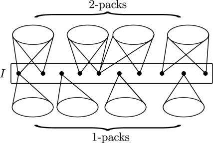
Figure 1: A schematic diagram showing the two kinds of packs. $I$ is a maximum independent set. Edges with end-points in different packs may be present in the graph; these are not shown in this diagram.

Lemma 9.

For any $1$-pack $V_{a}$, $G[V_{a}]$ is a clique.

Proof.

Assume we have $x,y\in V_{a}$, with $xy\not\in E$. Consider $(I\setminus\{a\})\cup\{x,y\}$. This is an independent set — $I\setminus\{a\}$ is independent, $x$ and $y$ have no edges to $I\setminus\{a\}$ from the definition of $V_{a}$, and there is no edge between them. But this set is larger than $I$, contradicting the definition of $I$. ∎

Lemma 10.

If there is an edge between a $2$-pack $V_{a,b}$ and a distinct pack $X$, then $X$ and $V_{a,b}$ have a common leg, i.e., $X=V_{a}$ or $X=V_{b}$ or $X=V_{a,c}$ or $X=V_{b,c}$ for some $c\in I$.

Proof.

Suppose not. Let $vw$ be the edge between $V_{a,b}$ and $X$, with $v\in V_{a,b}$ and $w\in X$. We know that $wa,wb\not\in E$, as $X$ has no common leg with $V_{a,b}$. Moreover, $ab\not\in E$ as they both belong to the independent set $I$, and $va,vb,vw\in E$ (first two from the definition of $V_{a,b}$, the third from the assumptions). Thus $G[\{v,w,a,b\}]$ is a claw, a contradiction. ∎

2.3 Solution structure

We now analyze how a MIDS can be placed with respect to $1$-packs and $2$-packs.

Lemma 11.

Let $v\in V$ and $w_{1},w_{2}\in N(v)$, $w_{1}w_{2}\notin E$. Then $N[v]\subseteq N[w_{1}]\cup N[w_{2}]$, i.e., $w_{1}$ and $w_{2}$ dominate everything that $v$ dominates.

Proof.

Assume there is a vertex $w_{3}\in N[v]\setminus(N[w_{1}]\cup N[w_{2}])$. We have $w_{1}\in N(v)$, so $v\in N[w_{1}]$ and so $w_{3}\neq v$. But now $w_{1}w_{2},w_{2}w_{3},w_{3}w_{1}\not\in E$, the first from the assumptions, the other two by the definition of $w_{3}$. On the other hand, $vw_{1},vw_{2},vw_{3}\in E$, thus $G[\{v,w_{1},w_{2},w_{3}\}]$ is a claw, a contradiction. ∎

Lemma 12.

Let $v_{1},v_{2}\in V$, $v_{1}v_{2}\notin E$. Let $w_{1},w_{2}\in N(v_{1})\cap N(v_{2})$, $w_{1}w_{2}\notin E$. Then $N[v_{1}]\cup N[v_{2}]=N[w_{1}]\cup N[w_{2}]$, i.e., $v_{1}$ and $v_{2}$ dominate together exactly the same vertex set as $w_{1}$ and $w_{2}$.

Proof.

Using Lemma 11 four times we obtain that $N[v_{1}],N[v_{2}]\subseteq N[w_{1}]\cup N[w_{2}]$ and $N[w_{1}],N[w_{2}]\subseteq N[v_{1}]\cup N[v_{2}]$. ∎

Lemma 13.

Assume there exists a MIDS $D$ and a pack $X$, such that $|D\cap X|>1$. Then there exists a MIDS $D^{\prime}$ that is not disjoint with $I$.

Proof.

By Lemma 9, all $1$-packs are cliques, so we cannot have two vertices from the independent set $D$ in $X$. Thus $X=V_{a,b}$ for some $a,b\in I$. Let $v,w\in D\cap X$. Now $vw\not\in E$ as $D$ is independent, $ab\not\in E$ as $I$ is independent, and $a,b\in N(v)\cap N(w)$ by the definition of $V_{a,b}$. Thus the assumptions of Lemma 12 are satisfied, and so $N[a]\cup N[b]=N[v]\cup N[w]$. Thus $D^{\prime}=(D\setminus\{v,w\})\cup\{a,b\}$ is a dominating set.

Now we apply Proposition 5. We have a dominating set $D^{\prime}$ with $|D^{\prime}|=|D|$, and an independent set $\{a,b\}\subseteq D^{\prime}$. Proposition 5 guarantees the existence of an independent dominating set $D^{\prime\prime}$ with $|D^{\prime\prime}|\leq|D^{\prime}|$ and $\{a,b\}\subseteq D^{\prime\prime}$. As $D$ was a MIDS, however, we have $|D^{\prime\prime}|\geq|D|$, and thus $|D^{\prime\prime}|=|D|$ — thus $D^{\prime\prime}$ is also a MIDS, and is not disjoint with $I$. ∎

Recall from the discussion at the end of Section 2.1 that we may assume, without loss of generality, that every MIDS in the graph $G$ is disjoint with the set $I$. It follows from Lemma 13 that every pack contains at most one vertex from the solution. We limit ourselves to this case in the remaining part of the algorithm.

Definition 14.

We say that a MIDS $D$ is compatible with a set $\mathcal{B}$ of packs, if $D$ contains exactly one vertex in each pack in $\mathcal{B}$, and no vertices in the packs not in $\mathcal{B}$.

Step 4.

The algorithm now guesses a set $\mathcal{B}$ of at most $k$ packs. From now on, the algorithm looks for a MIDS compatible with $\mathcal{B}$.

As the number of packs is at most $2k+\binom{2k}{2}=O(k^{2})$, we have $2^{O(k\log k)}$ possible guesses.

Some guesses are clearly invalid.

Step 5.

The algorithm discards guesses in which:

1. there exists a vertex $a\in I$ that cannot be dominated, i.e., no pack with leg $a$ is chosen to be in $\mathcal{B}$;

2. or there exists a vertex $a\in I$, such that at least three packs with leg $a$ are chosen to be in $\mathcal{B}$ (we cannot find three independent vertices in $N(a)$, as they would make a claw with the center in vertex $a$).

To sum up, for each $a\in I$ there exist one or two packs in $\mathcal{B}$ that have a leg $a$.

2.4 Algorithm structure

From now on, the algorithm maintains the partition of the vertex set $V$ into three parts:

1. $V^{\mathtt{Active}}$, vertices that can be chosen into the constructed MIDS, and we need to dominate them;

2. $V^{\mathtt{Passive}}$, vertices that cannot be chosen into the constructed MIDS, but we need to dominate them;

3. $V^{\mathtt{Done}}$, vertices that cannot be chosen into the constructed MIDS, and we somehow have ensured that they would be dominated, i.e., we do not need to care about them.

As we show later in this section (See Lemma 18), it turns out that it is sufficient to look for a solution which is “mostly” — and not necessarily totally — an independent set. More precisely, it is sufficient to find a “dominating candidate” which is also a dominating set:

Definition 15.

A set $D\subseteq V^{\mathtt{Active}}$ is called a dominating candidate if it satisfies the following properties:

1. $|D|=|\mathcal{B}|$ and $D$ consists of exactly one active vertex from each pack in $\mathcal{B}$;

2. if $X,Y\in\mathcal{B}$ and $X$ and $Y$ share a leg, then the two vertices in $D\cap(X\cup Y)$ are nonadjacent.

We say that the partition $(V^{\mathtt{Active}},V^{\mathtt{Passive}},V^{\mathtt{Done}})$ is safe if every dominating candidate dominates $V^{\mathtt{Active}}\cup V^{\mathtt{Done}}$.

Let $D$ be a dominating candidate, let $X,Y\in\mathcal{B}$, and let $x,y$ be the vertices in $X,Y$ respectively which are present in $D$. Further, let $xy$ be an edge in the graph. If $X$ is a $2$-pack, then by Lemma 10 the packs $X$ and $Y$ share a leg. The second condition in the definition of a dominating candidate then implies that there is no edge between $x$ and $y$, a contradiction. Thus both $X$ and $Y$ are $1$-packs. Therefore, while the subgraph induced by a dominating candidate may contain edges, any such edge is between vertices which belong to distinct $1$-packs. As we see in Lemma 18, this relaxation in the independence requirement for vertices drawn from $1$-packs helps in the justification of Step 8 below.

At the end of this section we obtain a state where the partition $(V^{\mathtt{Active}},V^{\mathtt{Passive}},V^{\mathtt{Done}})$ is safe.

Initially, $V^{\mathtt{Active}}$ consists of vertices in packs in $\mathcal{B}$, $V^{\mathtt{Done}}=I$ and $V^{\mathtt{Passive}}=V\setminus(I\cup V^{\mathtt{Active}})$ (we do not need to care about $I$, since we have discarded choices of $\mathcal{B}$ that do not dominate whole $I$). Thus, every dominating candidate dominates $V^{\mathtt{Done}}$, but not necessarily $V^{\mathtt{Active}}$. During the whole algorithm we shall keep the invariant that all active vertices are in $\bigcup\mathcal{B}$ and all passive vertices are in $V\setminus I\setminus\bigcup\mathcal{B}$.

In the following set of steps we assign some vertices to $V^{\mathtt{Done}}$ (keeping the invariant that every dominating candidate dominates $V^{\mathtt{Done}}$) and assure that every dominating candidate dominates $V^{\mathtt{Active}}$. This is formally justified in Lemma 18.

Lemma 16.

Let $v\in V_{a}\in\mathcal{B}$ and assume that $N[v]\subseteq N[a]$, i.e., $v$ knows only $a$ and vertices from packs that have leg $a$. Then, if there exists an MIDS $D$ compatible with $\mathcal{B}$ containing $v$, then there exists an MIDS $D^{\prime}$ of cardinality not larger than $D$ that is not disjoint with $I$.

Proof.

We proceed as in the proof of Lemma 13. Consider the set $D^{\prime}=(D\cup\{a\})\setminus\{v\}$. This is a dominating set, as $N[v]\subseteq N[a]$. As $\{a\}$ is an independent set, by Proposition 5 we can obtain a MIDS $D^{\prime\prime}$ not larger than $D^{\prime}$ (and thus not larger than $D$), which contains $a$. That ends the proof. ∎

This Lemma will be used in the justification of the following step:

Step 6.

For each $v\in V_{a}\in\mathcal{B}$ such that $N[v]\subseteq N[a]$, move $v$ to $V^{\mathtt{Done}}$.

We will now focus on packs that are alone in $\mathcal{B}$:

Definition 17.

A pack $X\in\mathcal{B}$ is called alone if for any leg $a$ of $X$ no other pack $Y\in\mathcal{B}$ has this leg.

Step 7.

Let $V_{a,b}\in\mathcal{B}$ be an alone $2$-pack in $\mathcal{B}$. For each vertex $v\in V_{a,b}$, if $V_{a,b}$ is not dominated by $v$, move $v$ to $V^{\mathtt{Done}}$.

Finally we remove several vertices from $V^{\mathtt{Passive}}$:

Step 8.

Let $X,Y\in\mathcal{B}$ be two packs that share a common leg $a\in I$. For each pack $Z\notin\mathcal{B}$ that has the leg $a$, move all vertices in $Z$ to $V^{\mathtt{Done}}$.

We justify all the above steps and formally prove that the current partition $(V^{\mathtt{Active}},V^{\mathtt{Passive}},V^{\mathtt{Done}})$ is safe in the following lemma:

Lemma 18.

Assume we have finished all steps up to Step 8.

1. $V^{\mathtt{Active}}\subseteq\bigcup\mathcal{B}$ and $V^{\mathtt{Passive}}\subseteq V\setminus(I\cup\bigcup\mathcal{B})$.

2. The partition $(V^{\mathtt{Active}},V^{\mathtt{Passive}},V^{\mathtt{Done}})$ is safe, i.e., every dominating candidate $D$ dominates $V^{\mathtt{Active}}\cup V^{\mathtt{Done}}$.

3. If there exists a MIDS $D$ compatible with $\mathcal{B}$, then there exists a dominating candidate that is a dominating set in $G$.

Proof.

The first claim is obvious, as in all above steps we only moved vertices from $V^{\mathtt{Active}}$ or $V^{\mathtt{Passive}}$ to $V^{\mathtt{Done}}$.

First note that in all of the above steps, we only transferred vertices into $V^{\mathtt{Done}}$, in particular if a vertex is in $V^{\mathtt{Active}}$, it had to be in $V^{\mathtt{Active}}$ at the start, and so is in one of the packs from $\mathcal{B}$. Consider any dominating candidate $D$, and any vertex $v\in V^{\mathtt{Active}}$. Let $X$ be the pack containing $v$. Observe that $X\in\mathcal{B}$, as $v\in V^{\mathtt{Active}}$ and all the vertices in packs not in $\mathcal{B}$ were outside $V^{\mathtt{Active}}$ from the beginning

Let $X=V_{a}$, i.e., let $X$ be a $1$-pack. This means $D$ contains a vertex $x\in V_{a}$, and — as $V_{a}$ is a clique by Lemma 9 — $v$ is dominated by $x$.

Now consider the case when $X=V_{a,b}$, i.e., $X$ is a $2$-pack. As before, $X\in\mathcal{B}$, and let $x$ be the vertex in $D\cap X$. As $D$ is a dominating candidate, $x\in V^{\mathtt{Active}}$. If $X$ is alone, then $x$ dominates $V_{a,b}$ — otherwise it would be removed from $V^{\mathtt{Active}}$ in Step 7 — and thus in particular $x$ dominates $v$. If $X$ is not alone, then we have another pack $Y\in\mathcal{B}$ that shares a leg, say $a$, with $X$, and a vertex $y\in Y\cap D$. As $D$ is a dominating candidate, $xy\not\in E$, and both $x$ and $y$ are adjacent to $a$. Thus, by Lemma 11, $\{x,y\}$ dominates $N[a]$, and — in particular — $v$.

The above proves that $V^{\mathtt{Active}}$ is indeed dominated by $D$. Now consider a vertex $v\in V^{\mathtt{Done}}$. If $v\in I$, then $v$ is dominated by every dominating candidate, as we disregarded choices of $\mathcal{B}$ that do not guarantee this in Step 5. We thus have to consider vertices moved to $V^{\mathtt{Done}}$ in Steps 6–8.

If $v$ was moved to $V^{\mathtt{Done}}$ in Step 6, then $v\in V_{a}$, with $V_{a}\in\mathcal{B}$. Thus there exists a vertex $x\in V_{a}\cap D$, and this vertex dominates $v$ as $V_{a}$ is a clique by Lemma 9.

If $v$ was moved to $V^{\mathtt{Done}}$ in Step 7, then $v\in V_{a,b}$, $V_{a,b}\in\mathcal{B}$ and $V_{a,b}$ was alone. Again, we have a vertex $x\in V_{a,b}\cap D$. The vertex $x$ is in $V^{\mathtt{Active}}$ as $D$ is a dominating candidate, so it had to survive Step 7 — thus it dominates $V_{a,b}$ and, in particular, $v$.

If $v$ was moved to $V^{\mathtt{Done}}$ in Step 8, we know that $v$ is in some pack $Z$ that shares a leg $a$ with two packs $X,Y\in\mathcal{B}$. Consider $x\in X\cap D$, $y\in Y\cap D$. We know $xy\not\in E$ as $D$ is a dominating candidate, and $x,y\in N(a)$. Thus, by Lemma 11, $\{x,y\}$ dominates $N[a]$, and, in particular, the vertex $v$.

Now for the third claim of the Lemma, consider a MIDS $D$ compatible with $\mathcal{B}$. It was a dominating candidate before we performed the steps 6–8. We want to prove that it is still a dominating candidate, i.e., that no vertex of $D$ was moved from $V^{\mathtt{Active}}$ to $V^{\mathtt{Done}}$ by any of the steps. In the case of Step 6 this follows from Lemma 16 and the branch we followed in Step 3. In the case of Step 8 the vertices were moved to $V^{\mathtt{Done}}$ from $V^{\mathtt{Passive}}$, which is disjoint with $D$.

Now assume $x\in D$ was moved to $V^{\mathtt{Done}}$ in Step 7. This means $x\in V_{a,b}$, where $V_{a,b}$ is alone in $\mathcal{B}$, and there exists a $v\in V_{a,b}$ that is not dominated by $x$. As $D$ is a dominating set, however, $v$ is dominated by some $y\in D$, $y\neq x$. By Lemma 10 the pack $Y$ that $y$ is in (which is distinct from $V_{a,b}$ as $x,y\in D$) has to share a leg with $V_{a,b}$, which contradicts with the assumption that $V_{a,b}$ is alone. ∎

Using Lemma 18, the algorithm now looks for a dominating candidate that is a dominating set in $G$. Note that a dominating candidate is a dominating set if and only if it dominates $V^{\mathtt{Passive}}$, since Lemma 18 ensures that the partition $(V^{\mathtt{Active}},V^{\mathtt{Passive}},V^{\mathtt{Done}})$ is safe (i.e., any dominating candidate always dominates $V^{\mathtt{Active}}\cup V^{\mathtt{Done}}$). In the following sections we reduce the sets $V^{\mathtt{Passive}}$ and $V^{\mathtt{Active}}$, sometimes by branching into a limited number of subcases. In each branching step the subcases cover all the possibilities for a dominating set which is a dominating candidate. Note that if at any step we decide that a vertex $v\in V^{\mathtt{Active}}$ will not be used in the solution, we may move it directly to $V^{\mathtt{Done}}$, as each dominating candidate dominates $v$ by the definition of a safe partition. In all steps, we shall only move vertices to $V^{\mathtt{Done}}$ from $V^{\mathtt{Active}}$ or $V^{\mathtt{Passive}}$, not between $V^{\mathtt{Active}}$ and $V^{\mathtt{Passive}}$. This provides us with the invariants $V^{\mathtt{Active}}\subseteq\bigcup\mathcal{B}$ and $V^{\mathtt{Passive}}\subseteq V\setminus(I\cup\bigcup\mathcal{B})$.

Let us introduce the following step.

Step 9.

If at any moment, for some $X\in\mathcal{B}$ we have $X\cap V^{\mathtt{Active}}=\emptyset$, we terminate this branch, as there are no dominating candidates. If at any moment, for some $v\in V^{\mathtt{Passive}}$ we have $N(v)\cap V^{\mathtt{Active}}=\emptyset$, we terminate this branch, as no dominating candidate dominates $v$.

If our instance has an MIDS of size at most $k$, then by the preceding arguments there exists a dominating candidate which is also a dominating set. We now fix one such (as yet unknown) dominating candidate which is a dominating set, and refer to it as the solution.

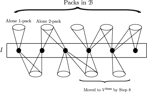
Figure 2: A snapshot of the graph after the application of Step 9. Edges with end-points in different packs are not shown.

2.5 Decomposition of $1$-packs

In this section we look into the structure of $1$-packs, i.e., sets $V_{a}$ for $a\in I$. Recall that each $G[V_{a}]$ is a clique by Lemma 9. Let $\mathtt{Packs}_{1}$ be the set of all $1$-packs.

Definition 19.

Let $V_{a}$ be a $1$-pack. We partition the vertices in $V_{a}$ into the following sets, depending on their neighbourhood in $\bigcup\mathtt{Packs}_{1}$

1. $\mathtt{T0}^{a}$ consists of those vertices $v\in V_{a}$ that do not know any other $1$-pack except for $V_{a}$, i.e., $N[v]\cap\bigcup\mathtt{Packs}_{1}\subseteq V_{a}$;

2. $\mathtt{T1}_{b}^{a}$ consists of those vertices $v\in V_{a}$ that know only $1$-packs $V_{a}$ and $V_{b}$ for $a\neq b\in I$, i.e., $N[v]\cap\bigcup\mathtt{Packs}_{1}\subseteq V_{a}\cup V_{b}$;

3. $\mathtt{T2}^{a}$ consists of all remaining vertices in $V_{a}$, i.e., those that know vertices from at least two $1$-packs other than $V_{a}$.

Naturally, the sets $\mathtt{T0}^{a}$, $\mathtt{T1}_{b}^{a}$ or $\mathtt{T2}^{a}$ may be empty. For example, if $V_{a}$ consists of a single vertex, it belongs to one of those sets and the other two are empty.

Note that Step 6 moved $\mathtt{T0}^{a}$ to $V^{\mathtt{Done}}$ for all $V_{a}\in\mathcal{B}$.

Now, for each $1$-pack $V_{a}\in\mathcal{B}$ we guess its part from which a vertex is taken to the solution.

Step 10.

For each $1$-pack $V_{a}\in\mathcal{B}$ guess one nonempty set $T\in\{\mathtt{T2}^{a}\}\cup\{\mathtt{T1}_{b}^{a}:b\in I,b\neq a\}$. The solution is only allowed to take a vertex from $T$, i.e., we move all vertices from $V_{a}\setminus T$ to $V^{\mathtt{Done}}$.

Note that there are $O(k)$ choices for each $1$-pack, so Step 10 leads to $2^{O(k\log k)}$ subcases.

Now we switch to analyzing sets $\mathtt{T2}^{a}$.

Lemma 20.

Let $\mathtt{T2}=\bigcup_{a\in I}\mathtt{T2}^{a}$. Let $G_{\mathtt{T2}}$ be the graph with vertex set $\mathtt{T2}$ and edge set consisting of those edges in $G[\mathtt{T2}]$ that have endpoints in different $1$-packs. Take two vertices $v,w\in\mathtt{T2}$, $v\in V_{a}$, $w\in V_{b}$, $a\neq b$. Then $v$ and $w$ are connected by an edge in $G$ (equivalently in $G_{\mathtt{T2}}$) if and only if $v$ and $w$ are in the same connected component of $G_{\mathtt{T2}}$.

Proof.

The forward implication is trivial. For the other direction, assume for the sake of contradiction that $v,w$ are in the same component of $G_{T2}$ but $vw\notin E$. Let $v=v_{0},v_{1},\ldots,v_{k}=w$ be a fixed shortest path in $G_{\mathtt{T2}}$ between $v$ and $w$. Let $V_{a_{i}}$ be the $1$-pack containing vertex $v_{i}$.

Note that $a_{i}v_{i},v_{i}v_{i-1},v_{i}v_{i+1}\in E$ and $a_{i}v_{i-1},a_{i}v_{i+1}\notin E$ (consecutive vertices on the path are in different $1$-packs by the definition of $G_{\mathtt{T2}}$). Thus we have $v_{i-1}v_{i+1}\in E$, as otherwise we have the claw $G[\{v_{i},a_{i},v_{i-1},v_{i+1}\}]$. If $a_{i-1}\neq a_{i+1}$, then $v_{i-1}v_{i+1}$ would be an edge in $G_{\mathtt{T2}}$ and the chosen path would not be the shortest. Thus, $a_{i}=a_{i+2}$ for all $0\leq i\leq k-2$, i.e., the path oscillates between two $1$-packs. Note that in this case $a_{1}=b$.

As $v\in\mathtt{T2}^{a}$, we have a neighbour $u$ of $v$ that is in different $1$-pack than $V_{b}$, say $u\in V_{c}$. We now prove by induction that $uv_{i}\in E$. The base of the induction is satisfied: $uv_{0}=uv\in E$. For the induction step, assume $uv_{i}\in E$. Then we risk the claw $G[\{v_{i},u,a_{i},v_{i+1}\}]$: $v_{i}u\in E$ (by the induction assumption), $v_{i}a_{i}\in E$, $v_{i}v_{i+1}\in E$, $ua_{i}\notin E$ as $c\neq a_{i}$ and $a_{i}v_{i+1}\notin E$ as $a_{i}\neq a_{i+1}$. Thus $uv_{i+1}\in E$.

Therefore $\{v_{0},v_{1},\ldots,v_{k}\}\subseteq N[u]\setminus N[c]$, and, by Lemma 4, $vw=v_{0}v_{k}\in E$. ∎

Lemma 21.

For any $1$-packs $V_{a}$, $V_{b}$, $a\not=b$ we have $N(\mathtt{T1}_{b}^{a})\cap V_{b}=\mathtt{T1}_{a}^{b}$ and $N(\mathtt{T2}^{a})\cap V_{b}\subseteq\mathtt{T2}^{b}$.

Proof.

Let $v\in\mathtt{T2}^{a}$ and let $v_{b}\in V_{b}\cap N(v)$, $a\neq b$. By the definition of $\mathtt{T2}^{a}$, $v$ has got neighbours in at least two $1$-packs other than $V_{a}$, so let $v_{c}\in V_{c}\cap N(v)$, $a\neq c\neq b$. We risk a claw $G[\{v,a,v_{b},v_{c}\}]$: $va,vv_{b},vv_{c}\in E$, $av_{b}\notin E$ and $av_{c}\notin E$. Thus $v_{b}v_{c}\in E$, $v_{b}\in\mathtt{T2}^{b}$ and $N(\mathtt{T2}^{a})\cap V_{b}\subseteq\mathtt{T2}^{b}$.

Now suppose there is a vertex $u$ which belongs to both $N(\mathtt{T1}_{b}^{a})$ and $\mathtt{T2}^{b}$. Then $u\in V_{b}$, there is a vertex $v\in\mathtt{T1}_{b}^{a}\subseteq V_{a}$ which is a neighbour of $u$, and $u$ sees a vertex $w$ which belongs to a $1$-pack $V_{c}$ which is different from both $V_{a}$ and $V_{b}$. Thus $uv,ub,uw\in E$. Since $v,w$ belong to $1$-packs other than $V_{b}$, neither of them sees $b$. Since $v\in\mathtt{T1}_{b}^{a}$, it does not see $w$ which is in a $1$-pack $V_{c}$ that is different from both $V_{a}$ and $V_{b}$. Thus $\{vb,bw,vw\}\cap E=\emptyset$, and so the vertex set $\{u,v,b,w\}$ induces a claw, a contradiction. Hence $N(\mathtt{T1}_{b}^{a})\cap\mathtt{T2}^{b}=\emptyset$.

Obviously $N(\mathtt{T1}_{b}^{a})\cap\mathtt{T0}^{b}=\emptyset$, so $N(\mathtt{T1}_{b}^{a})\cap V_{b}\subseteq\mathtt{T1}_{a}^{b}$. By symmetry, $N(\mathtt{T1}_{a}^{b})\cap V_{a}\subseteq\mathtt{T1}_{b}^{a}$. Since every vertex in $\mathtt{T1}_{a}^{b}$ has a neighbour in $V_{a}$, we have $N(\mathtt{T1}_{b}^{a})\cap V_{b}=\mathtt{T1}_{a}^{b}$. ∎

This leads us to the following definition:

Definition 22.

Take the graph $G_{\mathtt{T2}}$ from Lemma 20. The vertex set of any connected component of $G_{\mathtt{T2}}$ is called a cluster. By $\mathtt{Clusters}$ we denote the set of all clusters.

Observe that, in general, a $1$-pack $V_{a}$ can have nonempty intersections with more than one cluster. Note that by Lemma 20, each cluster induces a clique in $G$. The structure of clusters gives us good control on what can be dominated by a vertex in a cluster.

Corollary 23.

Let $v\in V_{a}$ be a vertex in a cluster $C$. Then $N[v]\setminus N[a]=C\setminus V_{a}$, i.e., vertex $v$ dominates the cluster $C$ and some neighbours of $a$.

Proof.

By Lemma 10, $v$ can have neighbours in $2$-packs with leg $a$ and in other $1$-packs. By Lemma 20 and Lemma 21, the set of neighbours of $v$ in other $1$-packs is exactly $C\setminus V_{a}$ and the corollary follows. ∎

We now move to $1$-packs outside $\mathcal{B}$. Let $V_{a}\notin\mathcal{B}$ and $V_{a}\cap V^{\mathtt{Passive}}\neq\emptyset$, i.e., $V_{a}$ was not moved to $V^{\mathtt{Done}}$ in Step 8. Then there exists exactly one pack in $\mathcal{B}$ with leg $a$, and it is a $2$-pack $V_{a,b}$ (since it is not $V_{a}$). Note that by Lemma 10 in any dominating candidate vertices in $\mathtt{T0}^{a}$ can be only dominated from the vertex in $V_{a,b}$, or else there would be a claw. For the same reason only $V_{a,b}$ can dominate $\mathtt{T1}_{c}^{a}$ if $V_{c}\notin\mathcal{B}$ or in Step 10 the algorithm did not guess the set $\mathtt{T1}_{a}^{c}$ for the $1$-pack $V_{c}$. Thus the following step leaves the algorithm in a safe state.

Step 11.

Let $V_{a}\notin\mathcal{B}$ and $V_{a}\cap V^{\mathtt{Passive}}\neq\emptyset$. Let $V_{a,b}$ be the unique pack in $\mathcal{B}$ with leg $a$. Let

$$\mathtt{T0ext}^{a}=\mathtt{T0}^{a}\cup\bigcup\{\mathtt{T1}_{c}^{a}:\mathtt{T1}_{a}^{c}\cap V^{\mathtt{Active}}=\emptyset\}.$$

Move to $V^{\mathtt{Done}}$ all vertices from $V_{a,b}\cap V^{\mathtt{Active}}$ that does not dominate all of $\mathtt{T0ext}^{a}$ (we cannot use them in the solution, since, by Lemma 10, only a vertex from $V_{a,b}$ can dominate $\mathtt{T0ext}^{a}$; recall that by Lemma 18 any dominating candidate dominates $V^{\mathtt{Active}}$, so we do not need to move them to $V^{\mathtt{Passive}}$). Move $\mathtt{T0ext}^{a}$ to $V^{\mathtt{Done}}$ (as it is now dominated by any vertex in $V_{a,b}\cap V^{\mathtt{Active}}$).

Let us analyze sets $\mathtt{T1}_{c}^{a}$ more deeply.

Lemma 24.

Let $V_{a}\notin\mathcal{B}$ and $V_{a}\cap V^{\mathtt{Passive}}\neq\emptyset$. Let $V_{a,b}$ be the unique pack in $\mathcal{B}$ with leg $a$. Assume that $v\in V_{a,b}$, $w\in\mathtt{T1}_{c}^{a}$, $vw\in E$ and $c\neq b$. Then $V_{a}\setminus\mathtt{T1}_{c}^{a}\subseteq N[v]$.

Proof.

Let $x$ be an arbitrary vertex in $N(w)\cap V_{c}$ and let $y$ be an arbitrary vertex in $V_{a}\setminus\mathtt{T1}_{c}^{a}$. As $wx,wy,wv\in E$ (recall that $G[V_{a}]$ is a clique), we risk a claw $G[\{w,v,x,y\}]$. Note that $vx\notin E$ due to Lemma 10 and $xy\notin E$, as $x\in\mathtt{T1}_{a}^{c}$ (Lemma 21) and $y\in V_{a}\setminus\mathtt{T1}_{c}^{a}$. Thus $vy\in E$. ∎

This leads us to the following step.

Step 12.

Let $V_{a}\notin\mathcal{B}$ and $V_{a}\cap V^{\mathtt{Passive}}\neq\emptyset$. Let $V_{a,b}$ be the unique pack in $\mathcal{B}$ with leg $a$. Assume that $\mathtt{T1}_{c}^{a}\cap V^{\mathtt{Passive}}$ is nonempty for at least one vertex $c\in I\setminus\{a,b\}$. Branch into following cases:

1. There exists $c\in I\setminus\{a,b\}$ such that the vertex in the solution from $V_{a,b}$ dominates at least one vertex from $\mathtt{T1}_{c}^{a}$. Guess $c$ (there are $O(k)$ choices). Move all vertices $v\in V_{a,b}$ with $N[v]\cap\mathtt{T1}_{c}^{a}=\emptyset$ to $V^{\mathtt{Done}}$. Move all vertices in $V_{a}\setminus\mathtt{T1}_{c}^{a}$ to $V^{\mathtt{Done}}$, as they are dominated by every vertex in $V_{a,b}\cap V^{\mathtt{Active}}$ by Lemma 24.

2. The vertex in the solution from $V_{a,b}$ does not dominate anything from $\mathtt{T1}_{c}^{a}$ for any $c\in I\setminus\{a,b\}$. Move all vertices in $V_{a,b}$ that do not satisfy this condition to $V^{\mathtt{Done}}$. Note that now, for each $c\in I\setminus\{a,b\}$, the vertices from $\mathtt{T1}_{c}^{a}$ can be dominated only by a vertex from $V_{c}$, as no vertex from $V_{a}$ is in the solution. Thus, for each $c\in I\setminus\{a,b\}$ we move to $V^{\mathtt{Done}}$ all vertices in $V_{c}\cap V^{\mathtt{Active}}$ that do not dominate all of $\mathtt{T1}_{c}^{a}$, and all vertices in $\mathtt{T1}_{c}^{a}$, as they are now guaranteed to be dominated.

Note that we move all vertices from $V^{\mathtt{Active}}$ directly to $V^{\mathtt{Done}}$ (not to $V^{\mathtt{Passive}}$) as they are guaranteed to be dominated by any dominating candidate by Lemma 18.

For each $1$-pack $V_{a}$ we have $O(k)$ choices, so the number of subcases here is $2^{O(k\log k)}$. We claim that at this point for each $V_{a}\notin\mathcal{B}$ we may have $\mathtt{T1}_{c}^{a}\cap V^{\mathtt{Passive}}\neq\emptyset$ for at most one choice of $c\in I\setminus\{a\}$. Indeed, if in Step 12 we have branched into the first case and guessed $c\in I\setminus\{a,b\}$, only $\mathtt{T1}_{c}^{a}$ may remain nonempty. Otherwise, only $\mathtt{T1}_{b}^{a}$ may remain nonempty.

We now aim to move sets $\mathtt{T2}^{a}\cap V^{\mathtt{Passive}}$ to $V^{\mathtt{Done}}$. The following lemma shows some more of the structure of clusters.

Lemma 25.

Let $V_{a}\notin\mathcal{B}$ and $V_{a}\cap V^{\mathtt{Passive}}\neq\emptyset$. Let $V_{a,b}$ be the unique pack in $\mathcal{B}$ with leg $a$. Assume that $\mathtt{T2}^{a}$ has vertices from at least two clusters. Then for each vertex $v\in V_{a,b}$ either $\mathtt{T2}^{a}\subseteq N[v]$ or $\mathtt{T2}^{a}\cap N[v]=\emptyset$.

Proof.

For the sake of a contradiction, assume that there exist $v\in V_{a,b}$ and $u,w\in\mathtt{T2}^{a}$, $vu\in E$, $vw\notin E$. W.l.o.g. we may assume that $u$ and $w$ lie in different clusters. Indeed, otherwise we have a vertex $z\in\mathtt{T2}^{a}$ that lies in a different cluster than $u$ and $w$. If $vz\in E$, we take $u:=z$, and if $vz\notin E$, we take $w:=z$.

Let $x$ be a neighbour of $u$ that lies in a $1$-pack different than $V_{a}$ and $V_{b}$ (there exists one by the definition of $\mathtt{T2}^{a}$). We have a claw $G[\{u,v,w,x\}]$: $uv,uw,ux\in E$ (recall that $G[V_{a}]$ is a clique), $vw\notin E$, $wx\notin E$ (as $w$ and $x$ are in different clusters and in different $1$-packs) and $vx\notin E$ (Lemma 10), a contradiction. ∎

This suggests the following branching:

Step 13.

Let $V_{a}\notin\mathcal{B}$ and $V_{a}\cap V^{\mathtt{Passive}}\neq\emptyset$. Let $V_{a,b}$ be the unique pack in $\mathcal{B}$ with leg $a$. Let $C_{1},C_{2},\ldots,C_{d}$ be clusters with vertices in $\mathtt{T2}^{a}$. Assume $d\geq 2$, i.e., $\mathtt{T2}^{a}$ has vertices from at least two clusters. We branch into two cases:

1. the vertex in the solution from $V_{a,b}$ dominates $\mathtt{T2}^{a}$; we move all vertices from $V_{a,b}\cap V^{\mathtt{Active}}$ that do not dominate $\mathtt{T2}^{a}$ to $V^{\mathtt{Done}}$ and move $\mathtt{T2}^{a}$ to $V^{\mathtt{Done}}$.

2. the vertex in the solution from $V_{a,b}$ does not dominate any vertex from $\mathtt{T2}^{a}$; we move all vertices from $V_{a,b}\cap V^{\mathtt{Active}}$ that dominate $\mathtt{T2}^{a}$ to $V^{\mathtt{Done}}$.

We can also similarly take care of $1$-packs that contain vertices from exactly one cluster:

Step 14.

Let $V_{a}\notin\mathcal{B}$ and $V_{a}\cap V^{\mathtt{Passive}}\neq\emptyset$. Let $V_{a,b}$ be the unique pack in $\mathcal{B}$ with leg $a$. Assume $\mathtt{T2}^{a}\neq\emptyset$ and $\mathtt{T2}^{a}\subseteq C$ for some cluster $C$. Branch into two cases:

1. the vertex in the solution from $V_{a,b}$ dominates $\mathtt{T2}^{a}$; as before, we move all vertices from $V_{a,b}\cap V^{\mathtt{Active}}$ that do not dominate $\mathtt{T2}^{a}$ to $V^{\mathtt{Done}}$ and move $\mathtt{T2}^{a}$ to $V^{\mathtt{Done}}$;

2. the vertex in the solution from $V_{a,b}$ does not dominate whole $\mathtt{T2}^{a}$. As before, we move all vertices from $V_{a,b}\cap V^{\mathtt{Active}}$ that dominate $\mathtt{T2}^{a}$ to $V^{\mathtt{Done}}$.

Let $C_{1},C_{2},\ldots,C_{d}$ be the clusters that are not disjoint with $V^{\mathtt{Passive}}$ after performing Steps 13 and 14. For each $1\leq i\leq d$ there exists a $1$-pack $V_{a_{i}}\notin\mathcal{B}$ and a $2$-pack $V_{a_{i},b_{i}}\in\mathcal{B}$ such that no vertex in $V_{a_{i},b_{i}}\cap V^{\mathtt{Active}}$ dominates whole $V_{a_{i}}\cap C_{i}\cap V^{\mathtt{Passive}}$. Thus, by Lemma 10, for each $i$ the solution takes at least one vertex from cluster $C_{i}$. This justifies the following branching rule:

Step 15.

If $d>k$, return NO from this branch, as clusters $C_{i}$ are pairwise disjoint. Otherwise, for each $1\leq i\leq d$ guess a distinct $1$-pack $B_{i}\in\mathcal{B}$ where the solution contains a vertex in $C_{i}$; move all vertices from $B_{i}\setminus C_{i}$ and $(C_{i}\setminus B_{i})\cap V^{\mathtt{Passive}}$ to $V^{\mathtt{Done}}$. We say that the $1$-pack $B_{i}$ is guessed to dominate $C_{i}$.

Note that in the above steps we move all vertices from $V^{\mathtt{Active}}$ directly to $V^{\mathtt{Done}}$ and not to $V^{\mathtt{Passive}}$, as they are dominated by any dominating candidate by Lemma 18. Note also that after performing Steps 13, 14 and 15, we have moved all sets $\mathtt{T2}^{a}$ to $V^{\mathtt{Done}}$.

Moreover, in Steps 13, 14 for each of $O(k)$ $1$-packs we have guessed one of two possible options, and in Step 15, for each of at most $k$ clusters we have guessed one of $O(k)$ possible options. This leaves us with $2^{O(k\log k)}$ branches after performing Steps 13, 14 and 15.

We now perform some cleaning.

Lemma 26.

Let $V_{c}\in\mathcal{B}$ be a $1$-pack with $V_{c}\cap V^{\mathtt{Active}}\subseteq\mathtt{T2}^{c}$, i.e., the algorithm guessed in Step 10 that the vertex from $V_{c}$ in the solution is contained in $\mathtt{T2}^{c}$. Assume that $V_{c}$ was not guessed to dominate any cluster in Step 15. Then if there exists a dominating candidate $D$ that dominates $V^{\mathtt{Passive}}$, then $D^{\prime}:=\{c\}\cup(D\setminus V_{c})$ is a dominating set in $G$.

Proof.

Since $D$ dominates $V^{\mathtt{Passive}}$, $D$ is a dominating set in $G$. Let $\{v\}=D\cap V_{c}$ and let $C$ be the cluster containing $v$ (recall that $D\subseteq V^{\mathtt{Active}}$ and $V_{c}\cap V^{\mathtt{Active}}\subseteq\mathtt{T2}^{c}$). To prove that $D^{\prime}$ is a dominating set in $G$ we need to ensure that $C\setminus V_{c}$ is dominated by $D\setminus\{v\}$ (recall Lemma 23).

Take $w\in C\setminus V_{c}$, let $w\in\mathtt{T2}^{a}$. If $V_{a}\in\mathcal{B}$, $w$ is dominated by a vertex from $D\cap V_{a}$. So let us assume that $V_{a}\notin\mathcal{B}$.

As Steps 13, 14 and 15 moved $\mathtt{T2}^{a}\cap V^{\mathtt{Passive}}$ to $V^{\mathtt{Done}}$, $w\in V^{\mathtt{Done}}$. We consider the possible steps in which vertex $w$ could have been placed placed in $V^{\mathtt{Done}}$. We moved vertices from $V^{\mathtt{Passive}}$ to $V^{\mathtt{Done}}$ in Step 8, Step 11, Step 12, Step 13, Step 14 and Step 15.

If $w$ was placed in $V^{\mathtt{Done}}$ in Step 8, $D\setminus\{v\}$ contains the two vertices in packs with leg $a$, and thus $w$ is dominated.

Step 11 does not touch the set $\mathtt{T2}^{a}$.

If $w$ was placed in $V^{\mathtt{Done}}$ in Step 12, then the algorithm guessed that it is dominated by a vertex from the $2$-pack $V_{a,b}$. As $v\notin V_{a,b}$, $D\setminus\{v\}$ dominates $w$.

Consider Steps 13, 14, and 15. In the $1$-pack $V_{a}$, we either guessed to dominate whole $\mathtt{T2}^{a}$ by a vertex from the $2$-pack $V_{a,b}\in\mathcal{B}$ or we guessed a $1$-pack $V_{d}$ ($d\neq c$) to dominate cluster $C$. As $v\notin V_{a,b}$ and $v\notin V_{d}$ respectively, $D\setminus\{v\}$ dominates $w$ in both cases. ∎

Lemma 26 implies that we can discard those subcases where there exists a $1$-pack $V_{c}$ which satisfies the conditions of the lemma : $V_{c}\in\mathcal{B}$, it was not guessed to dominate any cluster in Step 15, and $V_{c}\cap V^{\mathtt{Active}}\subseteq\mathtt{T2}^{c}$. Indeed, if in such a subcase there exists a solution, i.e., a dominating candidate $D$ that dominates $V^{\mathtt{Passive}}$, by Lemma 26 there exists a dominating set $D^{\prime}$ not disjoint with $I$. By Proposition 5 ($I_{D}=D^{\prime}\cap I$), there exists an MIDS not disjoint with $I$, a contradiction to the guess in Step 3.

Step 16.

If there exists a $1$-pack $V_{c}$ satisfying the conditions in Lemma 26, terminate the branch.

Let us conclude this section with the following lemma.

Lemma 27.

After executing Steps 10–16:

1. the algorithm is in a safe state;

2. if before Steps 10–16 there existed a dominating candidate that dominated $V^{\mathtt{Passive}}$, then after Steps 10–16 there exists one in at least one subcase or there exists an MIDS not disjoint with $I$;

3. we branched into at most $2^{O(k\log k)}$ subcases;

4. in every $1$-pack $V_{a}\notin\mathcal{B}$, the set $V_{a}\cap V^{\mathtt{Passive}}$ is empty or is contained in one set $\mathtt{T1}_{c}^{a}$;

5. in every $1$-pack $V_{a}\in\mathcal{B}$, the set $V_{a}\cap V^{\mathtt{Active}}$ is contained in one set $\mathtt{T1}_{b}^{a}$ or in one cluster in $\mathtt{T2}^{a}$.

Proof.

The first two claims were justified by the inline comments when steps were described.

The third claim can be seen as follows. In Step 10, in Step 11 and in Step 16 we do not branch. In Step 12 we have $O(k)$ subcases for each $1$-pack $V_{a}\notin\mathcal{B}$. As we have $O(k)$ $1$-packs, the bound holds for this step. The bound on the number of subcases introduced by Steps 13, 14, 15 has been justified after their descriptions.

As for the fourth claim, note that after Step 13 and Step 14, the sets $\mathtt{T2}^{a}$ are contained in $V^{\mathtt{Done}}$. Step 11 moved sets $\mathtt{T0}^{a}$ to $V^{\mathtt{Done}}$. Step 12 reduced the number of sets $\mathtt{T1}_{b}^{a}$ with passive vertices to at most one set.

The fifth claim follows directly from branching in Step 10 and from cleaning in Step 16. ∎

2.6 Auxiliary CSP and dynamic programming

We now define an auxiliary CSP problem and see that the current state of the algorithm is in fact an instance of this CSP.

Definition 28.

An instance of the auxiliary CSP consists of a set $\mathtt{Vars}$ of variables, for each variable $x\in\mathtt{Vars}$ a set of possible values $\mathtt{Val}(x)$, and a set of constraints $\mathtt{Cons}$. A constraint is a triple $C=(x_{C},y_{C},\mathtt{Allow}_{C})$, where $x_{C},y_{C}\in\mathtt{Vars}$, $x_{C}\neq y_{C}$ and $\mathtt{Allow}_{C}\subseteq\mathtt{Val}(x_{C})\times\mathtt{Val}(y_{C})$. The solution is an assignment $\phi$ that assigns to each $x\in\mathtt{Vars}$ a value $\phi(x)\in\mathtt{Val}(x)$ such that for each constraint $C=(x_{C},y_{C},\mathtt{Allow}_{C})$ we have $(\phi(x_{C}),\phi(y_{C}))\in\mathtt{Allow}_{C}$.

If an instance of the auxiliary CSP problem has a certain simple structure, then it can be solved in polynomial time.

Lemma 29.

If an auxiliary CSP instance has the property that for each $x\in\mathtt{Vars}$ there are at most $2$ other variables such that there exists constraints bounding $x$ and these variables, then the instance can be solved in polynomial time.

Proof.

Let $\mathcal{C}$ be an auxiliary CSP instance on a set $\mathtt{Vars}$ of variables which has the stated property. Let $\{x,y\}\subseteq\mathtt{Vars}$ be a set of two variables such that there is more than one constraint involving $x$ and $y$, and let these constraints be $\{(x,y,A_{1}),(x,y,A_{2}),\ldots,(x,y,A_{\ell})\}$. We may replace all these constraints by the single constraint $(x,y,\displaystyle{\bigcap_{i=1}^{\ell}A_{i}})$ to obtain an equivalent CSP instance. Also, one can merge two constraints $(x,y,A_{1})$ and $(y,x,A_{2})$ which differ only in the order of the variables, into a single constraint $(x,y,A_{12})$ in the natural manner. Therefore in the rest of the proof we assume, without loss of generality, that there is at most one constraint in the auxiliary CSP instance $\mathcal{C}$ which involves any given subset of two variables.

We represent $\mathcal{C}$ as a graph $\mathcal{G}$ on the vertex set $\mathtt{Vars}$ by adding, for each constraint $C=(x,y,\mathtt{Allow}_{C})$, an edge labelled $\mathtt{Allow}_{C}$ between the vertices $x$ and $y$. Observe that because of the special property of $\mathcal{C}$, this graph has maximum degree at most $2$, and so it is a collection of paths and cycles. For any vertex set $X\subseteq V(\mathcal{G})$, we define the “sub-instance” of $\mathcal{C}$ associated with $X$ to be the CSP instance consisting of the variable set $X$, the sets of possible values of the variables in $X$, and all the constraints of $\mathcal{C}$ which involve the variables in $X$. Note that, in general, the sub-instance associated with a vertex set $X$ may not be well-formed, in that it may contain constraints which involve variables which are not in $X$.

Let $A\subseteq V(\mathcal{G})$ be a set of vertices of $\mathcal{G}$ such that the subgraph induced by $A$ is a connected component of $\mathcal{G}$. Observe that the connectivity of $\mathcal{G}[A]$ ensures that for any variable $x\in A$, the set $\{y\in\mathtt{Vars}\,\mid\,(x,y,\mathtt{Allow}_{C})\in\mathtt{Cons}\}$ is a subset of $A$. So the sub-instance associated with $A$ is well-formed. Further, if $A_{1},A_{2},\ldots,A_{\ell}$ are the vertex sets of all the connected components of $\mathcal{G}$, and $\phi_{1},\phi_{2},\ldots,\phi_{\ell}$ are solutions to the sub-instances of $\mathcal{C}$ associated with $A_{1},A_{2},\ldots,A_{\ell}$, respectively, then $\phi=\phi_{1}\uplus\phi_{2}\ldots\uplus\phi_{\ell}$ is a solution of $\mathcal{C}$. Conversely, if $\phi$ is a solution of $\mathcal{C}$, then for any $1\leq i\leq\ell$, $\phi$ restricted to the variable set $A_{i}$ is clearly a solution of the sub-instance of $\mathcal{C}$ associated with $A_{i}$.

If the connected component induced by the vertex set $A$ is a path, say $(a_{1},a_{2},\ldots,a_{\ell})$, then we can find a solution for the sub-instance associated with $A$, if it exists, by “pruning the path”. We first associate, with each $a_{i}$, a list $L_{i}$ containing the set $\mathtt{Val}(a_{i})$ of possible values of $a_{i}$. For each $2\leq i\leq\ell$ in this order, we go through the list $L_{i}$ and delete all those values $y\in L_{i}$ for which there is no $x\in L_{i-1}$ such that $(x,y)\in\mathtt{Allow}_{C};(a_{i-1},a_{i},\mathtt{Allow}_{C})\in\mathtt{Cons}$. Observe that after this step, for each value $y\in L_{i}$ there is at least one value $x\in L_{i-1}$ such that assigning the values $x$ to $a_{i-1}$ and $y$ to $a_{i}$ satisfies the constraint involving $a_{i-1}$ and $a_{i}$.

If this procedure deletes all the values in any list $L_{i}$, then there is no solution for the sub-instance associated with $A$, and so also for the CSP instance $\mathcal{C}$. Otherwise, this sub-instance has at least one solution. To find such a solution, pick any surviving value $x_{\ell}\in L_{\ell}$. Now for each $\ell-1\geq i\geq 1$, in this order, find a value $x_{i}\in L_{i}$ such that assigning the values $x_{i}$ to $a_{i}$ and $x_{i+1}$ to $a_{i+1}$ satisfies the constraint involving $a_{i}$ and $a_{i+1}$. Such a value $x_{i}$ always exists, and the assignment which gives the value $x_{i}$ to $a_{i}$ for each $1\leq i\leq\ell$ satisfies all the constraints involving the variables of $A$.

If the connected component induced by the vertex set $A$ is a cycle, say $(a_{1},a_{2},\ldots,a_{\ell},a_{1})$, then we guess a value — say $x$ — for the variable $a_{2}$ and check whether there is a solution for the sub-instance associated with $A$ which gives the value $x$ to $a_{2}$. To do this, we delete the vertex $a_{2}$ from $A$ to obtain a path, and associate, with each remaining $a_{i}$, a list $L_{i}$ containing the set $\mathtt{Val}(a_{i})$ of possible values of $a_{i}$. From the list $L_{1}$ we delete all those values $y$ for which $(y,x)\notin\mathtt{Allow}_{C};(a_{1},a_{2},\mathtt{Allow}_{C})\in\mathtt{Cons}$. Similarly, from the list $L_{3}$ we delete all those values $y$ for which $(x,y)\notin\mathtt{Allow}_{C};(a_{2},a_{3},\mathtt{Allow}_{C})\in\mathtt{Cons}$. We now prune the path $(a_{3},a_{4},\ldots,a_{\ell},a_{1})$ in the same way as before, starting with these values for the lists $L_{i}$.

We solve for each connected component of $\mathcal{G}$ in this manner. If any component does not have a solution, then we stop the processing and return NO as the answer. Otherwise we return the disjoint union of the satisfying assignments computed for each component.

Since the possible set of values and the set of constraints are both part of the input, a straightforward implementation of the pruning operation takes $O(n^{3})$ time over all component paths where $n$ is the size of the input. Also, a value for a variable can be guessed in $O(n)$ time, and so a simple implementation of the above algorithm solves the problem in $O(n^{4})$ time. ∎

Before we start to encode the state of our algorithm, we need one more step.

Step 17.

Let $v\in V^{\mathtt{Passive}}$. Assume that $N(v)\cap V^{\mathtt{Active}}\subseteq X$ for one pack $X\in\mathcal{B}$. Then $v$ can be dominated only by the single vertex from the solution from $X$, so move to $V^{\mathtt{Done}}$ the vertex $v$ and all vertices from $X\cap V^{\mathtt{Active}}$ that do not dominate $v$. Note that by Lemma 18 all vertices in $X\cap V^{\mathtt{Active}}$ are dominated by any dominating candidate, so we can move them directly to $V^{\mathtt{Done}}$ instead of $V^{\mathtt{Passive}}$.

Observe that after performing Step 17 exhaustively, each vertex from $V^{\mathtt{Passive}}$ has neighbours in at least two packs from $\mathcal{B}$ (recall that by Step 9 each vertex in $V^{\mathtt{Passive}}$ has at least one neighbour in $V^{\mathtt{Active}}$). This can be streghtened to the following observation.

Lemma 30.

Assume we have executed Step 17 exhaustively. Let $W$ be a pack not in $\mathcal{B}$ and assume that $W\cap V^{\mathtt{Passive}}\neq\emptyset$. Then there exist two packs $Y,Z\in\mathcal{B};Y\neq Z$ such that every vertex $v\in W\cap V^{\mathtt{Passive}}$ has got neighbours in $Y\cap V^{\mathtt{Active}}$, in $Z\cap V^{\mathtt{Active}}$ and no other active neighbours in other packs in $\mathcal{B}$. Moreover, if a pack $Y^{\prime}\in\mathcal{B}$ shares a leg with $W$, then $Y^{\prime}\in\{Y,Z\}$.

Proof.

As Step 17 cannot be executed more, each vertex $v\in W\cap V^{\mathtt{Passive}}$ has active neighbours in at least two packs in $\mathcal{B}$. Thus, we need to prove that the active neighbours of $v$ are contained in only two packs from $\mathcal{B}$.

Firstly assume that $W$ is a $1$-pack, $W=V_{a}$. As $W$ was not moved to $V^{\mathtt{Done}}$ in Step 8, there exists exactly one pack in $\mathcal{B}$ with leg $a$, denote it by $V_{a,b}$ (it is not a $1$-pack, since it is not $V_{a}$). Moreover, by Lemma 27, $V_{a}\cap V^{\mathtt{Passive}}$ is contained in one set $\mathtt{T1}_{c}^{a}$. Thus, $v$ has active neighbours only in $V_{a,b}$ and $V_{c}$.

Now assume that $W$ is a $2$-pack, $W=V_{a,b}$. As $W$ was not moved to $V^{\mathtt{Done}}$ in Step 8, there exists exactly one pack in $\mathcal{B}$ with leg $a$ (say $X_{a}$) and exactly one pack in $\mathcal{B}$ with leg $b$ (say $X_{b}$). Observe that $X_{a}\neq X_{b}$ as otherwise $X_{a}=X_{b}=W$. Moreover, by Lemma 10, $W$ does not have edges to any other pack in $\mathcal{B}$. Thus, $v$ has active neighbours only in $X_{a}$ and $X_{b}$. ∎

Informally, Lemma 30 implies that every pack not in $\mathcal{B}$ which still contains some nontrivial vertices (i.e., those in $V^{\mathtt{Passive}}$) implies a constraint on only two packs in $\mathcal{B}$.

Using Lemma 30 we now show how to encode the state of our algorithm after all the steps from previous sections have been performed. Recall that we have $V^{\mathtt{Active}}\subseteq\bigcup\mathcal{B}$ and $V^{\mathtt{Passive}}\subseteq V\setminus(I\cup\bigcup\mathcal{B})$, as we had so in Lemma 18 and we only performed moves from $V^{\mathtt{Active}}$ or $V^{\mathtt{Passive}}$ to $V^{\mathtt{Done}}$.

Definition 31.

The auxiliary CSP associated with partition $(V^{\mathtt{Active}},V^{\mathtt{Passive}},V^{\mathtt{Done}})$ is constructed as follows.

1. For each pack $X\in\mathcal{B}$ we introduce variable $x^{X}$ with set of values $V^{\mathtt{Active}}\cap X$.

2. For each pair of packs $X,Y\in\mathcal{B}$ with a common leg $a$ we introduce the constraint

   $$(x^{X},x^{Y},\{(v,w)\in(X\cap V^{\mathtt{Active}})\times(Y\cap V^{\mathtt{Active}}):vw\notin E\}).$$

   This constraint is called an independence constraint.

3. For each pack $W\notin\mathcal{B}$ that has nontrivial vertices, i.e., $W\cap V^{\mathtt{Passive}}\neq\emptyset$ take the two packs $Y$ and $Z$ from Lemma 30 and we introduce the constraint

   $$(x^{Y},x^{Z},\{(v,w)\in(Y\cap V^{\mathtt{Active}})\times(Z\cap V^{\mathtt{Active}}):W\cap V^{\mathtt{Passive}}\subseteq N[v]\cup N[w]\}).$$

   This constraint is called a dominating constraint.

The following Lemma formalizes the equivalence of the constructed auxiliary CSP and the current state of the algorithm.

Lemma 32.

There exists a dominating candidate $D$ that is a dominating set in $G$ if and only if the associated auxiliary CSP has got a solution.

Proof.

Let $D$ be a dominating candidate that is a dominating set in $G$. For each $x^{X}\in\mathtt{Vars}$ define $\phi(x)$ to be the unique vertex in $D\cap X$. Since $D$ is a dominating candidate, $\phi$ satisfies all independence constraints. Since $D$ is a dominating set in $G$, in particular it dominates $V^{\mathtt{Passive}}$ and $\phi$ satisfies all dominating constraints. Thus, $\phi$ is a solution to the auxiliary CSP instance.

In the other direction, let $\phi$ be a solution to the auxiliary CSP instance. We prove that $D=\{\phi(x):x\in\mathtt{Vars}\}$ is a dominating candidate that dominates $G$.

By the definition of the auxiliary CSP instance, $D$ contains exactly one vertex from each pack in $\mathcal{B}$, thus $D$ is compatible with $\mathcal{B}$. The independence constraints imply that the second property from the dominating candidate definition is satisfied also.

The dominating constraints imply that $D$ dominates $V^{\mathtt{Passive}}$. As the algorithm is in a safe state, this implies that $D$ dominates $G$. ∎

We have constructed the above CSP, but the multigraph associated with it can have arbitrarily large degree. The next section is devoted to bounding the maximum degree of the associated multigraph in order to use Lemma 29.

2.7 CSP degree reduction

In this last part of the algorithm we bound the maximum degree of the multigraph associated with the auxiliary CSP problem by $2$, so that we can solve it in polynomial time as explained in Lemma 29.

Before we start, we need to do some cleaning.

Step 18.

For each pack $W$ satisfying $W\notin\mathcal{B}$ and $W\cap V^{\mathtt{Passive}}\neq\emptyset$ and for each pack $X\in\mathcal{B}$ that satisfies $N(X\cap V^{\mathtt{Active}})\cap W\cap V^{\mathtt{Passive}}\neq\emptyset$ guess whether the vertex in $X$ from the solution dominates something from $W$ or it dominates nothing from $W$. In both cases, move the vertices from $X\cap V^{\mathtt{Active}}$ that do not satisfy the chosen case to $V^{\mathtt{Done}}$. Moreover, in the second case, apply Step 17 to pack $W$, as then $W\cap V^{\mathtt{Passive}}$ can be dominated by only one pack in $\mathcal{B}$ (Lemma 30).

Note that by Lemma 30, for each such $W$ there exist exactly two packs $X$. There are $O(k^{2})$ packs, thus the Step 18 leads to $2^{O(k^{2})}$ subcases.

After the above cleaning the following holds.

Lemma 33.

Assume that Step 18 is performed exhaustively and let $C$ be a dominating constraint in the associated auxiliary CSP instance that corresponds to a pack $W\notin\mathcal{B}$, $W\cap V^{\mathtt{Passive}}\neq\emptyset$. Let $Y$ and $Z$ be the packs asserted by Lemma 30. Then each vertex in $(Y\cup Z)\cap V^{\mathtt{Active}}$ has at least one neighbour in $W$.

Proof.

If $W\cap V^{\mathtt{Passive}}\neq\emptyset$, then both $Y$ and $Z$ guessed in Step 18 to dominate something from $W$. Thus, only vertices with neighbours in $W\cap V^{\mathtt{Passive}}$ survived in $V^{\mathtt{Active}}$ in Step 18. ∎

We now present the crucial structural lemma that allows us to reduce the auxiliary CSP instance.

Lemma 34.

Let $a\in I$ and $X,W_{1},W_{2}$ be three packs with leg $a$ satisfying $X\in\mathcal{B}$, $W_{1},W_{2}\notin\mathcal{B}$, $W_{1}\cap V^{\mathtt{Passive}}\neq\emptyset$, $W_{2}\cap V^{\mathtt{Passive}}\neq\emptyset$. Moreover, assume that the following property holds: for each pack $A\in\{X,W_{1},W_{2}\}$, for each vertex $v\in A\cap(V^{\mathtt{Active}}\cup V^{\mathtt{Passive}})$ there exists a vertex $n_{v}\in V\setminus(X\cup W_{1}\cup W_{2})$ such that $N(n_{v})\cap(X\cup W_{1}\cup W_{2})\subseteq A$. Then $(X\cup W_{1}\cup W_{2})\cap(V^{\mathtt{Active}}\cup V^{\mathtt{Passive}})$ can be partitioned into two sets $K_{1}$ and $K_{2}$, such that $G[K_{1}]$ and $G[K_{2}]$ are cliques and if $v_{1}\in K_{1}$, $v_{2}\in K_{2}$ and $v_{1}$ and $v_{2}$ are in different packs, then $v_{1}v_{2}\notin E$. Such sets $K_{1}$ and $K_{2}$ can be found in polynomial time.

Proof.

Let $V_{H}=(X\cup W_{1}\cup W_{2})\cap(V^{\mathtt{Passive}}\cup V^{\mathtt{Active}})$ and let $H$ be a graph with vertex set $V_{H}$ and with edge set $E_{H}$ consisting of those edges of $G[V_{H}]$ that have endpoints in different packs. We prove that the graph $H$ has at most two connected components, and a vertex set of each connected component of $H$ induces a clique in $G$.

By Lemma 30, every vertex in $(W_{1}\cup W_{2})\cap V^{\mathtt{Passive}}$ has a neighbour in $X\cap V^{\mathtt{Active}}$. By Lemma 33, every vertex in $X\cap V^{\mathtt{Active}}$ has a neighbour in $W_{1}\cap V^{\mathtt{Passive}}$ and a neighbour in $W_{2}\cap V^{\mathtt{Passive}}$. Thus, every connected component of $H$ intersects all three packs $X$, $W_{1}$ and $W_{2}$.

Moreover, by Lemma 4, for each $v\in V_{H}$ we have that $G[N[v]\setminus N[n_{v}]]$ is a clique. Note that $N_{H}(v)\subseteq N[v]\setminus N[n_{v}]$. Thus we have a following observation: if a vertex $v\in V_{H}$ has two neighbours in the two other packs, then they are adjacent.

We now prove the following claim. Let $C$ be a vertex set of a connected component in $H$ and let $v\in C\cap X$ be an arbitrary vertex. Then $C\cap(W_{1}\cup W_{2})\subseteq N[v]$. By the contrary, assume that there exists $w\in W_{1}\cap V^{\mathtt{Passive}}\cap C$, such that $vw\notin E$. Let $v=v_{0},v_{1},v_{2},\ldots,v_{k}=w$ be the shortest path in $H$ between $v$ and $w$; if $vw\notin E$ then $k\geq 2$. If for some $i$ the vertices $v_{i-1}$, $v_{i}$, $v_{i+1}$ lie in three different packs $X$, $W_{1}$, $W_{2}$, by the previous observation they form a triangle: $v_{i-1}$ and $v_{i+1}$ are neighbours of $v_{i}$ and they lie in the two other packs, so $v_{i-1}v_{i+1}\in E$. Thus the path is not the shortest one. Therefore, the path oscillates between $X$ and $W_{1}$, i.e., $v_{2i}\in X$ and $v_{2i+1}\in W_{1}$. Let $u\in W_{2}\cap V^{\mathtt{Passive}}$ be an arbitrary neighbour of $v$ in $H$. Then, by induction we prove that $v_{i}u\in E$ for every $i$: $v_{0}u=vu\in E$ and if $v_{i-1}u\in E$, then $v_{i}$ and $u$ are neighbours of $v_{i-1}$ and they lie in different packs, thus $v_{i}u\in E$. Thus $wu,vu\in E$ and $u$, $v$, $w$ lie in different packs, so $vw\in E$ and the claim is proven.

Now let $v_{1},v_{2}$ be two vertices in the same connected component $C$ of $H$ and assume $v_{1}$ and $v_{2}$ lie in the same pack. As $C$ has vertices in each pack $X$, $W_{1}$, and $W_{2}$, let $u$ be a common neighbour in $H$ of $v_{1}$ and $v_{2}$ that lie in a different pack (it exists by the previous claim). Recall than $N[u]\setminus N[n_{u}]$ induces a clique and $v_{1},v_{2}\in N[u]\setminus N[n_{u}]$, thus $v_{1}v_{2}\in E$. Thus $G[C]$ is a clique.

Assume that there are three different connected components $C_{1}$, $C_{2}$, $C_{3}$ in $H$. Take $v_{1}\in C_{1}\cap X$, $v_{2}\in C_{2}\cap W_{1}$, $v_{3}\in C_{3}\cap W_{2}$. We have $av_{1},av_{2},av_{3}\in E$ but $v_{1}v_{2},v_{2}v_{3},v_{3}v_{1}\notin E$, a contradiction, as $G[\{a,v_{1},v_{2},v_{3}\}]$ is a claw.

Thus $H$ consists of one or two connected components. If one, we take $K_{1}=V_{H}$ and $K_{2}=\emptyset$. If two, we take $K_{1}$ and $K_{2}$ to be equal to the vertex sets of these components. This completes the proof. Note that the sets $K_{1}$ and $K_{2}$ can be computed in polynomial time, since they are simply the connected components of the graph $H$. ∎

Let us note that the conditions in Lemma 34 can be checked in polynomial time: for each vertex $v\in(X\cup W_{1}\cup W_{2})\cap(V^{\mathtt{Passive}}\cup V^{\mathtt{Active}})$ we simply check all possibilities for $n_{v}$.

Note that the above lemma gives us the following step.

Step 19.

For each triple of packs $X\in\mathcal{B}$; $W_{1},W_{2}\notin\mathcal{B}$ check whether the conditions of Lemma 34 are satisfied. If yes, compute sets $K_{1}$ and $K_{2}$ and guess whether the vertex in the solution from the pack $X$ is in $K_{1}$ or $K_{2}$. If the set $K_{i}$ is chosen, move vertices from $K_{3-i}\cap X$ to $V^{\mathtt{Done}}$ (not to $V^{\mathtt{Passive}}$, as Lemma 18 asserts that all dominating candidates dominate $V^{\mathtt{Active}}$), move vertices from $(W_{1}\cup W_{2})\cap K_{i}\cap V^{\mathtt{Passive}}$ to $V^{\mathtt{Done}}$ (they are guaranteed to be dominated by the vertex in $X$), and apply Step 17 to the vertices in $(W_{1}\cup W_{2})\cap K_{3-i}\cap V^{\mathtt{Passive}}$ (now they cannot be dominated by the vertex from $X$).

Let us note that the above step moves sets $W_{1}\cap V^{\mathtt{Passive}}$ and $W_{2}\cap V^{\mathtt{Passive}}$ to $V^{\mathtt{Done}}$.

Lemma 35.

Assume Step 19 has been executed for sets $X$, $W_{1}$ and $W_{2}$. Then $(W_{1}\cup W_{2})\cap V^{\mathtt{Passive}}=\emptyset$, i.e., $W_{1}$ and $W_{2}$ no longer give raise to a dominating constraint in the auxiliary CSP.

Proof.

Before Step 19 is executed on $X$, $W_{1}$ and $W_{2}$, each vertex in $(W_{1}\cup W_{2})\cap V^{\mathtt{Passive}}$ was in $K_{1}$ or $K_{2}$. Assume that $K_{i}$ is chosen to contain the vertex from the solution in $X$. Then the vertices from $(W_{1}\cup W_{2})\cap V^{\mathtt{Passive}}\cap K_{i}$ are moved to $V^{\mathtt{Done}}$, since they are dominated by any vertex in $X\cap V^{\mathtt{Active}}$. Moreover, the vertices from $(W_{1}\cup W_{2})\cap V^{\mathtt{Passive}}\cap K_{3-i}$ are moved to $V^{\mathtt{Done}}$ in the execution of Step 17, since now they can be dominated only by vertices from one particular pack in $\mathcal{B}$. ∎

Let us now note that Step 19 cannot be executed many times.

Lemma 36.

Step 19 can be executed at most $O(k^{2})$ times, and thus all executions lead to at most $2^{O(k^{2})}$ subcases.

Proof.

If Step 19 is executed on packs $X$, $W_{1}$ and $W_{2}$, then $W_{1}\cap V^{\mathtt{Passive}}$ and $W_{2}\cap V^{\mathtt{Passive}}$ become empty. Thus each pack not in $\mathcal{B}$ can be touched by Step 19 at most once. As there are $O(k^{2})$ packs, the bound follows. ∎

We finish the algorithm with the following reasoning.

Lemma 37.

Assume in the auxiliary CSP instance there is a variable $x^{X}$ such that there are at least three other variables $Y$ bounded with $X$ by a constraint (i.e., the variable $x^{X}$ has at least $3$ neighbours in the multigraph associated with the auxiliary CSP instance). Then there exists packs $W_{1}$ and $W_{2}$ such that the triple $(X,W_{1},W_{2})$ satisfy conditions for Lemma 34, i.e., it is eligible for the reduction in Step 19.

Proof.

We consider several subcases. In the reasoning below, we often look at various packs $W\notin\mathcal{B}$, such that $W\cap V^{\mathtt{Passive}}\neq\emptyset$ and $X\cap V^{\mathtt{Active}}$ can dominate $W$, i.e., $W$ gives a dominating constraint that involve $X$. By the second dominator for $W$ we mean the second pack $X^{\prime}\in\mathcal{B}$ asserted by Lemma 30.

Case 1. $X$ is a $2$-pack, $X=V_{a,b}$. Then $X$ can dominate only packs with leg $a$ or $b$ (Lemma 10) and can be connected by independence constraints to other packs with leg $a$ or $b$. Recall that by Step 5 there is at most one independence constraint per leg of $X$.

Case 1.1. $X$ is connected by independence constraints to two other packs $X_{a}$ and $X_{b}$, where $X_{a}$ has leg $a$, and $X_{b}$ has leg $b$. By Step 8, all packs not in $\mathcal{B}$ with leg $a$ or $b$ were moved to $V^{\mathtt{Done}}$, thus these two independence constraints are the only constraints that involve $X$.

Case 1.2. $X$ is connected by independence constraints to one pack $X_{a}$ that shares leg $a$ with $X$. By Step 8, all packs not in $\mathcal{B}$ with leg $a$ were moved to $V^{\mathtt{Done}}$. By the assumptions of the lemma, there are at least two packs $W_{1}$ and $W_{2}$ that have leg $b$, are not in $\mathcal{B}$ and $W_{1}\cap V^{\mathtt{Passive}}\neq\emptyset$ and $W_{2}\cap V^{\mathtt{Passive}}\neq\emptyset$, i.e., $W_{1}$ and $W_{2}$ induce dominating constraints. Moreover, we can assume that the second dominators of $W_{1}$ and $W_{2}$ are different and different than $X_{a}$, as $X$ has at least three neighbours in the multigraph associated with the auxiliary CSP instance.

Case 1.2.1. Both $W_{1}$ and $W_{2}$ are $2$-packs, $W_{1}=V_{b,c}$, $W_{2}=V_{b,d}$. Note that $a\neq c\neq d\neq a$. Thus, $X$, $W_{1}$ and $W_{2}$ satisfy conditions for Step 19, where $a$ is the private neighbour of all the vertices in $X$, $c$ is the private neighbour for $W_{1}$ and $d$ for $W_{2}$.

Case 1.2.2. $W_{1}$ is a $1$-pack, $W_{1}=V_{b}$ and $W_{2}$ is a $2$-pack, $W_{2}=V_{b,d}$. Recall Lemma 27: $W_{1}\cap V^{\mathtt{Passive}}\subseteq\mathtt{T1}_{c}^{b}$ for some $1$-pack $V_{c}\in\mathcal{B}$. In other words, the $1$-pack $V_{c}$ is the second dominator for $W_{1}$. As the second dominator of $W_{1}$ is different than $X_{a}$, $X_{a}\neq V_{c}$ and $c\neq a$. Note that there exists at most one pack $X_{d}\in\mathcal{B}$ with leg $d$, as otherwise $W_{2}=V_{b,d}$ would be moved to $V^{\mathtt{Done}}$ by Step 8. Moreover, $X_{d}$ is the second dominator for $W_{2}$. We infer that, as the second dominators for $W_{1}$ and $W_{2}$ are different, $X_{d}\neq V_{c}$ and $c\neq d$. Obviously $d\neq a$. Thus, by Lemma 10, $V_{c}$ has no neighbours in $X$ nor $W_{2}$ and the triple $(X,W_{1},W_{2})$ satisfy the condition for Step 19: the private neighbour for vertices in $X$ is $a$, for $W_{2}$ is $d$, and each vertex in $W_{1}\cap V^{\mathtt{Passive}}\subseteq\mathtt{T1}_{c}^{b}$ has a neighbour in $V_{c}$.

Case 1.3. There are no independence constraints involving $X$, i.e., $X$ is an alone $2$-pack in $\mathcal{B}$. By the assumptions of the lemma, for at least one leg of $X$ (say $b$) we have at least two packs $W_{1}$ and $W_{2}$ sharing leg $b$ with $W_{1}\cap V^{\mathtt{Passive}}\neq\emptyset$, $W_{2}\cap V^{\mathtt{Passive}}\neq\emptyset$.

Case 1.3.1 Both $W_{1}$ and $W_{2}$ are $2$-packs, $W_{1}=V_{b,c}$, $W_{2}=V_{b,d}$. As $a,c,d$ are pairwise different, $X$, $W_{1}$ and $W_{2}$ satisfy conditions for Step 19 similarly as in Case 1.2.1.

Case 1.3.2 $W_{1}=V_{b}$ is a $1$-pack and $W_{2}=V_{b,d}$ is a $2$-pack. Similarly as in Case 1.2.2, $W_{1}\cap V^{\mathtt{Passive}}\subseteq\mathtt{T1}_{c}^{b}$ and $a,c,d$ are pairwise different ($V_{a}\notin\mathcal{B}$ as $X$ is alone in $\mathcal{B}$). Thus $X$, $W_{1}$ and $W_{2}$ satisfy conditions for Step 19.

Case 2. $X=V_{a}$ is a $1$-pack.

Case 2.1. $X$ is connected by an independence constraint with a pack $X^{\prime}=V_{a,b}$. Then, by Step 8, all packs not in $\mathcal{B}$ with leg $a$ were moved to $V^{\mathtt{Done}}$. Recall that by Lemma 26 the algorithm either guessed that the vertex in the solution from $V_{a}$ dominates some cluster, or is contained in $\mathtt{T1}_{c}^{a}$ for some $1$-pack $V_{c}\notin\mathcal{B}$. In the first case $V_{a}$ is not bounded by any dominating constraint. In the second case it is bounded by one constraint, induced by $V_{c}$. Thus, $X$ can be involved in at most two constraints.

Case 2.2. $X$ is an alone $1$-pack in $\mathcal{B}$, i.e. it does not share legs with other packs from $\mathcal{B}$. Note that by Lemma 27, $X\cap V^{\mathtt{Active}}\subseteq\mathtt{T1}_{b}^{a}$ for some pack $V_{b}$ or $X\cap V^{\mathtt{Active}}\subseteq C$ for some cluster $C$.

Case 2.2.1. $X\cap V^{\mathtt{Active}}\subseteq\mathtt{T1}_{b}^{a}$. By the assumptions of the lemma, there exist two packs $W_{1},W_{2}\notin\mathcal{B}$ with leg $a$ that induce a dominating constraint involving $X$. Moreover, we can assume that the second dominator for $V_{b}$, $W_{1}$ and $W_{2}$ are pairwise different. Let $W_{1}=V_{a,c}$, $W_{2}=V_{a,d}$. Observe that $b\neq c\neq d\neq b$: clearly $c\neq d$ and $b$ must be different from both of them, because otherwise the second dominator of $V_{b}$ would be equal to the second dominator of $W_{1}$ or $W_{2}$. Therefore, by Lemma 10, $V_{b}$ do not have neighbours in $W_{1}$ nor $W_{2}$. Thus $X$, $W_{1}$ and $W_{2}$ satisfy the conditions in Step 19: for $W_{1}$ and $W_{2}$ we take $c$ and $d$ as private neighbours, and each vertex in $X\cap V^{\mathtt{Active}}$ has a neighbour in $V_{b}$.

Case 2.2.2. $X\cap V^{\mathtt{Active}}\subseteq C$ for some cluster $C$. Assume that $C\cap V_{b}\neq\emptyset$ and $C\cap V_{c}\neq\emptyset$ for some $1$-packs $V_{b}$ and $V_{c}$ (recall that a cluster has vertices in at least three $1$-packs). Assume in contrary, that the claim does not hold. Then there are at least three packs $W_{1},W_{2},W_{3}\notin\mathcal{B}$ with leg $a$ — no other $1$-pack gives raise to a dominating constraint involving $X$ as $X$ was guessed to dominate cluster $C$. Let $W_{i}=V_{a,d_{i}}$ for $i=1,2,3$. As there are at least three such packs, we can number them so that $d_{1}\neq b$ and $d_{2}\neq b$. Then $V_{b}$ does not have neighbours in $W_{1}$ and $W_{2}$ and $X$, $W_{1}$ and $W_{2}$ satisfy the conditions of Step 19: for $W_{i}$ we take $d_{i}$ as an universal private neighbour and each vertex in $X\cap V^{\mathtt{Active}}$ has a neighbour in cluster $C$ in $V_{b}$. ∎

Corollary 38.

If Step 19 cannot be performed, the multigraph associated with the auxiliary CSP instance has maximum degree at most $2$ and it can be solved in polynomial time as in Lemma 29.

The above corollary finishes the proof of Theorem 1.

2.8 Summary

We end this section by repeating the main ideas of the algorithm. This subsection should not be read as an introduction to the algorithm, but rather — as the whole algorithm is at the same time rather complex and rather technical — as a tool to help the reader who followed the details to grasp the large picture.

There are two crucial steps we begin with. The first is noting that we can look for an MIDS instead of a MDS (Proposition 5) — or rather, look for a MDS but only in the branches containing a MIDS. The second is noticing that we can begin with the largest independent set, and assume that our solution is disjoint from it (otherwise we branch on the intersection — this is Step 1 and Step 3). Note that this trick could be done with any other set with size bounded by $f(k)$ that can be found in FPT-time, the fact that this is the maximal independent set is not used here.

After these two steps we can introduce packs, $1$-packs and $2$-packs. We assume the reader who read through the whole proof is familiar with the terms by now. One important reason this is going to be useful is that our solution will contain at most one vertex from each pack (this is Lemma 13) — thus, we have in some sense localized the solution — there are few packs (few meaning $f(k)$, independent of $n$), so we will be able to branch over the set of packs. We use this idea immediately in steps 4 and 5 to localize the solution even further.

To get a general idea of what happens next it is good to think about the auxiliary CSP now. The idea is that for each pack containing a vertex of the solution we have up to $n$ ways to choose this vertex. We think of this as of choosing a valuation for the packs (the values being the particular vertices), and we try to see what constraints are imposed by the fact we are looking for a MIDS.

We obtain two types of constraints — independence and domination. The independence constraints are always binary (that is, they always tie together only two packs). There are, however, too many of them — note that when looking for a MIDS we have an independence constraint between any two $1$-packs. Here we use a technical trick — we relax our assumptions, and instead of looking for a MIDS we look for a dominating candidate (see Definition 15), which basically means we drop the independence constraints between $1$-packs.

One may ask here — why do we not drop all the independence constraints, if it is so easy? The answer is that assuming that the solution vertices from two packs that share a leg are independent helps us in proving domination (for instance in the justification of Step 8), while we will be able to control the remaining independence constraints in Lemma 37.

The situation is more involved with domination constraints. As each vertex of the graph has to be dominated, we have $n$ domination constraints. Moreover, a priori a vertex can be dominated from any of the packs — thus the constraints are not even binary to begin with. Thus, to even define the CSP graph, we need to deal with this problem.

To deal with the domination constraints we introduce the partition of $V$ into the sets $V^{\mathtt{Active}}$, $V^{\mathtt{Passive}}$ and $V^{\mathtt{Done}}$. Each vertex moved to $V^{\mathtt{Done}}$ means a domination constraint removed, each vertex removed from $V^{\mathtt{Active}}$ is a possible value of one variable removed, and — at the same time — the reduction of the set of possible dominating candidates (and thus the possibility of performing further reductions).

The easy part are the vertices from $\mathcal{B}$. After some preliminary steps we were able to show (Lemma 18) that they will be dominated by any dominating candidate. Thus, they do not introduce any constraints (or, to look at it in a different way, after discarding some values of the variables that can be proved to be unnecessary, the domination constraints imposed by these vertices are trivial).

The medium-easy part are the vertices from $2$-packs. A vertex of a $2$-pack that would introduce a constraint on more that two variables is automatically dominated — this is stated in Lemma 30, but follows from the simple observations around Lemmata 10 and 11, used in the justification of Step 8.

The difficult part are the vertices in $1$-packs that will be dominated by other $1$-packs. Here a whole classification needs to be developed, to check what can each $1$-pack vertex dominate, culminating in Lemma 27, which strongly localizes the vertices in $1$-packs. It helps to understand what actually made the $1$-packs so problematic. It is mainly that while we can pretty well control what vertices can dominate a vertex from a $2$-pack (they have to come from a pack that shares a leg with the $2$-pack, and after Step 8 only two of them are left), the $1$-packs can actually be all connected to one another, and as each has only one leg, it is more difficult to find claws in them. And the structure is indeed more complicated than in the case of $2$-packs.

It turns out, however, that if a $1$-pack has edges into at least two other $1$-packs, we have enough information to form claws easily, and force a strong structure (this is the $\mathtt{T2}$ case, Lemma 20) — the clusters. We analyze the clusters to show that they do not dominate each other (Corollary 23), and thus, in particular, there cannot be more than $k$ of them, so we will be able to branch upon which pack dominates each cluster (Step 13). On the other hand if there is only one $1$-pack adjacent to the given one, we can branch over all possible cases (Step 10).

After reducing all the constraints to be binary we are almost done.

Now we bound the degree of each vertex by $2$, which turns out to be rather simple, although somewhat tedious. Instead of repeating similar arguments over and over again, we show a general framework (in Lemma 34 and Step 19), and then apply it multiple times in Lemma 37.

3 Hardness in $t$-claw-free graphs

In this section we prove Theorem 2, i.e., we show that the Dominating Set problem is $W[2]$-hard on graph classes characterized by the exclusion of the $t$-claw as an induced subgraph, for any $t\geq 4$. This implies that the problem is unlikely to have FPT algorithms on these classes of graphs [13]. We prove the hardness result for the class of $4$-claw-free graphs; note that this implies the result for all $t\geq 4$. To prove that Dominating Set is $W[2]$-hard on this class, we present a parameterized reduction from the Red-Blue Dominating Set problem, which is known to be $W[2]$-hard [14]. A direct reduction eluded us, however, and so we make use of an intermediate, coloured version of the problem:

Colourful Red-Blue Dominating Set
Input:	A bipartite graph $G=(R\uplus B,E)$, $k\in\mathbb{N}$, and a colouring function $c:R\to\{1,2,\ldots,k\}$
Parameter:	$k$
Question:	Does there exist a set $D\subseteq R$ of $k$ distinctly coloured vertices such that $D$ is a dominating set of $B$?

We call such a dominating set $D$ a colourful red-blue dominating set of $G$. This coloured version turns out to be at least as hard as the original problem:

Lemma 39.

The Colourful Red-Blue Dominating Set problem is $W[2]$-hard.

Proof.

We reduce from the Red-Blue Dominating Set problem which is known to be $W[2]$-hard [14], and which is defined as follows:

Red-Blue Dominating Set
Input:	A bipartite graph $G=(R\uplus B,E)$, $k\in\mathbb{N}$
Parameter:	$k$
Question:	Does there exist a set $D\subseteq R$ of size $k$ such that $D$ is a dominating set of $B$?

Such a set $D$ is called a red-blue dominating set of $G$. Observe that the above problem is equivalent to asking if there is a red-blue dominating set of size at most $k$, which is how this problem is usually phrased. If $|R|<k$, then the problem instance is easily solved (say YES if and only if there are no isolated vertices in $B$), so we can assume without loss of generality that $|R|\geq k$. If there is a red-blue dominating set of size at most $k$, we can always pad it up with enough vertices to obtain a red-blue dominating set of size exactly $k$, and the converse is trivial.

Given an instance $(G=(R\uplus B,E),k)$ of Red-Blue Dominating Set, we create a new graph $G^{\prime}$ whose vertex set consists of the set $B$ and $k$ copies $R_{1},R_{2},\ldots,R_{k}$ of the set $R$. For each vertex $v\in R$, we make the neighbourhood of each copy of $v$ in $G^{\prime}$ identical to the neighbourhood of $v$ in $G$; the edge set $E^{\prime}$ of $G^{\prime}$ can be thought of as $k$ disjoint copies of the edge set of $G$. We set $R^{\prime}=R_{1}\cup R_{2}\cup\cdots\cup R_{k}$. For each $1\leq i\leq k$, the colouring function $c$ maps all vertices in $R_{i}$ to the colour $i$. This completes the construction; the reduced instance is $(G^{\prime}=(R^{\prime}\cup B,E^{\prime}),k,c)$. See Figure 3.

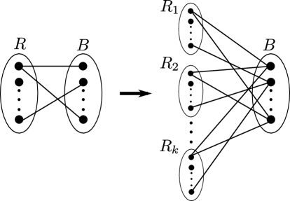
Figure 3: Reduction from Red-Blue Dominating Set to Colourful Red-Blue Dominating Set. Each set $R_{i}$ is a copy of $R$, and its vertices have a distinct colour.

If $(G,k)$ is a YES instance of Red-Blue Dominating Set, then let $D=\{v_{1},v_{2},\ldots,v_{k}\}\subseteq R$ be a dominating set of $B$ of size $k$. For $1\leq i,j\leq k$, let $v_{i}^{j}$ denote the copy of $v_{i}$ in the set $R_{j}$ in $G^{\prime}$. It is not difficult to verify that the set $\{v_{i}^{i}\mid 1\leq i\leq k\}$ is a colourful red-blue dominating set of $G^{\prime}$ of size $k$.

Conversely, let $(G^{\prime},k)$ be a YES instance of Colourful Red-Blue Dominating Set. Then there exists a set of vertices $D=\{v_{1},v_{2},\ldots,v_{k};v_{i}\in R_{i}\}$ which dominates all vertices in $B$, in $G^{\prime}$. Let $D^{\prime}=\{v\in R\mid D\text{ contains a copy of }v\}$. Then $D^{\prime}$ contains at most $k$ vertices, and it is straightforward to verify that $D^{\prime}$ dominates $B$ in $G$. ∎

We are now ready to show the main result of this section:

Lemma 40.

The Dominating Set problem restricted to $4$-claw-free graphs is $W[2]$-hard.

Proof.

We reduce from the Colourful Red-Blue Dominating Set problem, which we show to be $W[2]$-hard in Lemma 39. Given an instance $(G=(R\uplus B,E),k,c)$ of Colourful Red-Blue Dominating Set, we construct an instance of Dominating Set on $4$-claw-free graphs as follows. We add all possible edges among the vertices in $B$ so that $B$ induces a clique. In the same way, we make $R$ a clique, and for each colour class (set of vertices for which $c$ assigns the same colour) $R_{i};1\leq i\leq k$ of $R$, we add a new vertex $v_{i}$ and make $v_{i}$ adjacent to all the vertices in $R_{i}$. We remove all colours from the vertices, and this completes the construction. See Figure 4.

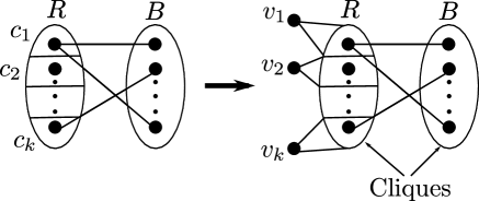
Figure 4: Reduction from Colourful Red-Blue Dominating Set to Dominating Set on $4$-claw-free graphs. The sets $R,B$ are both made cliques, and a new vertex is made global to each colour class.

Let $G^{\prime}$ be the graph obtained. It is easy to verify that the neighbourhood of each vertex in $G^{\prime}$ is a union of at most three vertex-disjoint cliques, and so $G^{\prime}$ is a $4$-claw-free graph; $(G^{\prime},k)$ is the reduced instance of Dominating Set on $4$-claw-free graphs.

If $(G,k,c)$ is a YES instance of Colourful Red-Blue Dominating Set, then let $D=\{u_{1},u_{2},\ldots,\newline u_{k};u_{i}\in R_{i}\}$ be a colourful dominating set of $B$ of size $k$. Since we did not delete any edge in constructing $G^{\prime}$ from $G$, the set $D$ dominates all of $B$ in $G^{\prime}$. Since we made the set $R$ a clique in $G^{\prime}$, the set $D$ dominates all of $R$ in $G^{\prime}$. Since each new vertex that we added to $G$ is adjacent to every vertex in some colour class, the set $D$ dominates all the newly added vertices in $G^{\prime}$ as well. Thus $D$ is a dominating set of $G^{\prime}$, of size $k$.

Conversely, if $(G^{\prime},k)$ is a YES instance of Dominating Set, then let $D=\{u_{1},u_{2},\ldots,u_{k}\}$ be a dominating set of $G^{\prime}$ of size $k$ in $G^{\prime}$. Since the neighbourhood in $G^{\prime}$ of each new vertex $v_{i}$ is the set $R_{i}$, $D\cap(R_{i}\cup\{v_{i}\})\neq\emptyset$. Since the sets $R_{i}\cup\{v_{i}\};1\leq i\leq k$ are pairwise vertex-disjoint, $D$ contains exactly one vertex from each set $R_{i}\cup\{v_{i}\}$, and no other vertex. Suppose $D\cap(R_{i}\cup\{v_{i}\})=v_{i}$ for some $i$. Then we can replace $v_{i}$ with an arbitrary vertex $x\in R_{i}$, in $D$, and this $D$ would still be a dominating set of $G^{\prime}$. This is because the neighbourhood $R_{i}$ of $v_{i}$ is a clique, and so $x\in R_{i}$ dominates all of $R_{i}$. Thus we can assume without loss of generality that $D$ contains no vertex $v_{i}$. Thus $D\subseteq R$ is a set of $k$ vertices, one from each set $R_{i}$, that dominates all vertices in $G^{\prime}$. Since we did not modify any adjacency between the sets $R$ and $B$ to construct $G^{\prime}$ from $G$, it follows that in $G$ the set $D$ dominates all vertices in $B$. Hence $D$ is a colourful red-blue dominating set of $G$ of size k. ∎

In the Connected Dominating Set (resp. Dominating Clique) problem, the input consists of a graph $G$ and $k\in\mathbb{N}$, the parameter is $k$, and the question is whether $G$ has a dominating set $D$ of size at most $k$ such that the subgraph of $G$ induced by the set $D$ is connected (resp. a clique). Observe that the reduction in Lemma 40 ensures that if the reduced graph $G^{\prime}$ has a dominating set of size at most $k$, then it has a dominating set $D^{\prime}$ of size at most (in fact, exactly) $k$ which induces a clique in $G^{\prime}$. Thus the above reduction also shows that

Corollary 41.

The Connected Dominating Set problem and the Dominating Clique problem are $W[2]$-hard when restricted to $4$-claw-free graphs.

Remark 42.

Observe that if a graph $G$ contains a $t^{\prime}$-claw $T^{\prime}$ for any $t^{\prime}\in\mathbb{N}$, $G$ also contains a $t$-claw $T$ for each $t\leq t^{\prime};t\in\mathbb{N}$. Indeed, each such $T$ occurs in $G$ as an induced subgraph of $T^{\prime}$. Taking the contrapositive, a $t$-claw-free graph is also $t^{\prime}$-claw-free for all $t^{\prime}\geq t;t,t^{\prime}\in\mathbb{N}$. It follows that the hardness results stated in Lemma 40 and Corollary 41 extend to $t$-claw-free graphs for all $t\geq 4$.

4 The Clique problem in claw-free graphs

In this section we prove Theorem 3, i.e., we give an FPT algorithm for the Clique problem in $t$-claw-free graphs.

The (decision version of the) Maximum Clique problem takes as input a graph $G$ and a positive integer $k$, and asks whether $G$ contains a clique (complete graph) on at least $k$ vertices as a subgraph. This is one of Karp’s original list of 21 NP-complete problems [27], and the standard parameterized version Clique, defined below, is a fundamental $W[1]$-complete problem [14]. The $W[1]$-hardness of Clique implies that the problem is unlikely to have FPT algorithms [13].

The classical decision variant of this problem remains NP-hard on claw-free graphs [18, Theorem 5.4]. In this section we show that, in contrast, the problem becomes easier from the point of view of parameterized complexity when we restrict the input to claw-free graphs.

Lemma 43.

For any $t\in\mathbb{N}$, the Clique problem is FPT on $t$-claw-free graphs, and can be solved in $(k+t-2)^{(t-1)(k-1)}n^{O(1)}$ time.

Proof.

We use Ramsey’s theorem for graphs, which states that for any two positive integers $i,c$, there exists a positive integer $\mathcal{R}(i,c)$ such that any graph on at least $\mathcal{R}(i,c)$ vertices contains either an independent set on $i$ vertices or a clique on $c$ vertices (or both) as an induced subgraph. Further, it is known [26] that $\mathcal{R}(i,c)\leq{{i+c-2}\choose{c-1}}$. Setting $i=t,c=k$, it follows that if a graph on at least ${{k+t-2}\choose{k-1}}={{k+t-2}\choose{t-1}}\leq(k+t-2)^{t-1}$ vertices does not contain an independent set of size $t$, then it must contain a clique on $k$ vertices.

Let $G$ be a $t$-claw-free input graph for the Clique problem, and let $v$ be any vertex in $G$. Since $G$ is $t$-claw-free, the neighbourhood of $v$ contains no independent set of size $t$. If $v$ has degree at least $(k+t-2)^{t-1}$, it then follows from Ramsey’s theorem that the neighbourhood of $v$ contains a clique on $k$ vertices. Hence, if any vertex in $G$ has degree $(k+t-2)^{t-1}$ or more, our FPT algorithm returns YES; this check can clearly be done in polynomial time.

Assume therefore that every vertex in the input graph has degree less than $(k+t-2)^{t-1}$. Our algorithm iterates over each vertex $v$ of degree at least $k-1$, and checks if its neighbourhood $N(v)$ contains a clique of size $k-1$. Observe that this procedure will find a $k$-clique in $G$ if it exists.

To check if $N(v)$ contains a clique of size $k-1$, the algorithm enumerates all $(k-1)$-sized subsets of $N(v)$ and checks whether any of these subsets induces a complete subgraph in $G$. There are ${|N(v)|\choose{k-1}}\leq{{(k+t-2)^{t-1}}\choose{k-1}}\leq(k+t-2)^{(t-1)(k-1)}$ such subsets, and these can be enumerated in $O((k+t-2)^{(t-1)(k-1)})$ time [16]. For each subset, it is sufficient to check if all ${{k-1}\choose 2}\leq k^{2}$ possible edges are present, which, given an adjacency matrix for $G$, can be done in $O(k^{2})$ time. Putting all these together, our algorithm solves the problem in $(k+t-2)^{(t-1)(k-1)}n^{O(1)}$ time. ∎

5 Conclusions

We derive an FPT algorithm for the Dominating Set problem parameterized by solution size, on graphs that exclude the claw $K_{1,3}$ as an induced subgraph. Our algorithm starts off using a maximum independent set of the input graph, known to be computable in polynomial time [28, 32]. We show that it is sufficient to look for an independent dominating set of the prescribed size. Our algorithm then uses the claw-freedom of the input graph to implement reduction rules which narrow down the possible ways in which a small dominating set could be present in the graph. Once these rules have been exhaustively applied, we are left with a graph and a set of constraints which must be satisfied by every dominating set of small size, where the constraints are highly structured in that they define an underlying graph of small degree. We then use dynamic programming on this underlying graph to retrieve the dominating set (or to find that no such dominating set could exist). The algorithm uses $2^{O(k^{2})}n^{O(1)}$ time and polynomial space to check if a claw-free graph on $n$ vertices has a dominating set of size at most $k$.

The most general class of graphs for which an FPT algorithm was previously known for this parameterization of Dominating Set is the class of $K_{i,j}$-free graphs, which exclude, for some fixed $i,j\in\mathbb{N}$, the complete bipartite graph $K_{i,j}$ as a (not necessarily induced) subgraph [31]. To the best of our knowledge, every other class for which an FPT algorithm was previously known for this parameterization of Dominating Set can be expressed as a subset of $K_{i,j}$-free graphs for suitably chosen values of $i$ and $j$. If $i=1$, then $K_{i,j}$-free graphs are graphs of bounded degree, on which the Dominating Set problem is easily seen to be FPT. For the interesting case when $i,j\geq 2$, the class of claw-free graphs and any class of $K_{i,j}$-free graphs are not comparable with respect to set inclusion: a $K_{i,j}$-free graph can contain a claw, and a claw-free graph can contain a $K_{i,j}$ as a subgraph. In this paper, we thus break new ground: we extend the range of graphs over which this parameterization of Dominating Set is known to be fixed-parameter tractable, beyond graph classes which can be described as $K_{i,j}$-free.

In addition to this main result, we also show that the Dominating Set problem is $W[2]$-hard (and therefore unlikely to have FPT algorithms) in $t$-claw-free graphs for any $t\geq 4$, and that the Clique problem is FPT in $t$-claw-free graphs for any $t\in\mathbb{N}$.

In the version of this paper which we submitted to ArXiv [10], we had stated:

“These results open up many new challenges. The most immediate open question is to get a faster FPT algorithm with a more reasonable running time; ideally, an algorithm that runs in $O^{\star}(c^{k})$ time for some small constant $c$. Another open problem, and perhaps of greater significance, is to find a polynomial kernel for the problem in claw-free graphs, or to show that no such kernel is likely to exist.”

Both these problems were later solved by Hermelin et al. [25]. Building on the structural characterization for claw-free graphs developed recently by Chudnovsky and Seymour [3, 4, 5, 6, 7, 8], they derive an FPT algorithm for the $k$-Dominating Set problem on claw-free graphs which runs in $9^{k}n^{O(1)}$ time. They also show that the problem has a polynomial kernel on $O(k^{4})$ vertices on claw-free graphs.

As mentioned above, $K_{i,j}$-free and claw-free graphs are two largest classes for which we now have FPT algorithms for Dominating Set. For what other classes of graphs, not contained in these two classes, is the problem FPT? Finally, is there an even larger class, which subsumes both claw-free and $K_{i,j}$-free graphs, for which the problem is FPT?

Acknowledgements.

We would like to thank anonymous referees for their valuable comments.

References

- [1] Noga Alon and Shai Gutner. Linear time algorithms for finding a dominating set of fixed size in degenerated graphs. Algorithmica, 54(4):544–556, 2009.
- [2] Ayelet Butman, Danny Hermelin, Moshe Lewenstein, and Dror Rawitz. Optimization problems in multiple-interval graphs. ACM Transactions on Algorithms, 6(2), 2010.
- [3] Maria Chudnovsky and Paul D. Seymour. Claw-free graphs. I. Orientable prismatic graphs. J. Comb. Theory, Ser. B, 97(6):867–903, 2007.
- [4] Maria Chudnovsky and Paul D. Seymour. Claw-free graphs. II. Non-orientable prismatic graphs. J. Comb. Theory, Ser. B, 98(2):249–290, 2008.
- [5] Maria Chudnovsky and Paul D. Seymour. Claw-free graphs. III. Circular interval graphs. J. Comb. Theory, Ser. B, 98(4):812–834, 2008.
- [6] Maria Chudnovsky and Paul D. Seymour. Claw-free graphs. IV. Decomposition theorem. J. Comb. Theory, Ser. B, 98(5):839–938, 2008.
- [7] Maria Chudnovsky and Paul D. Seymour. Claw-free graphs. V. Global structure. J. Comb. Theory, Ser. B, 98(6):1373–1410, 2008.
- [8] Maria Chudnovsky and Paul D. Seymour. Claw-free graphs VI. Colouring. J. Comb. Theory, Ser. B, 100(6):560–572, 2010.
- [9] Bruno Courcelle. Graph rewriting: An algebraic and logic approach. In Handbook of Theoretical Computer Science, Volume B: Formal Models and Sematics (B), pages 193–242. 1990.
- [10] Marek Cygan, Geevarghese Philip, Marcin Pilipczuk, Michal Pilipczuk, and Jakub Onufry Wojtaszczyk. Dominating set is fixed parameter tractable in claw-free graphs. CoRR, abs/1011.6239, 2010.
- [11] Anuj Dawar, Martin Grohe, and Stephan Kreutzer. Locally excluding a minor. In LICS, pages 270–279. IEEE Computer Society, 2007.
- [12] Anuj Dawar and Stephan Kreutzer. Domination problems in nowhere-dense classes. In Ravi Kannan and K Narayan Kumar, editors, IARCS Annual Conference on Foundations of Software Technology and Theoretical Computer Science (FSTTCS 2009), volume 4 of Leibniz International Proceedings in Informatics (LIPIcs), pages 157–168, Dagstuhl, Germany, 2009. Schloss Dagstuhl–Leibniz-Zentrum fuer Informatik.
- [13] Rodney G. Downey and Michael R. Fellows. Fixed parameter tractability and completeness. In Complexity Theory: Current Research, pages 191–225, 1992.
- [14] Rodney G. Downey and Michael R. Fellows. Parameterized Complexity. Springer, 1999.
- [15] Zdenek Dvorak, Daniel Král, and Robin Thomas. Deciding first-order properties for sparse graphs. In FOCS, pages 133–142. IEEE Computer Society, 2010.
- [16] Gideon Ehrlich. Loopless algorithms for generating permutations, combinations, and other combinatorial configurations. Journal of the ACM, 20(3):500–513, 1973.
- [17] John A. Ellis, Hongbing Fan, and Michael R. Fellows. The dominating set problem is fixed parameter tractable for graphs of bounded genus. J. Algorithms, 52(2):152–168, 2004.
- [18] Ralph Faudree, Evelyne Flandrin, and Zdenĕk Ryjác̆ek. Claw-free graphs — A Survey. Discrete Mathematics, 164:87–147, 1997.
- [19] Jörg Flum and Martin Grohe. Fixed-parameter tractability, definability, and model-checking. SIAM J. Comput., 31(1):113–145, 2001.
- [20] Jörg Flum and Martin Grohe. Parameterized Complexity Theory. Springer-Verlag, 2006.
- [21] Fedor V. Fomin and Dimitrios M. Thilikos. Dominating sets in planar graphs: Branch-width and exponential speed-up. SIAM J. Comput., 36(2):281–309, 2006.
- [22] Markus Frick and Martin Grohe. Deciding first-order properties of locally tree-decomposable structures. J. ACM, 48(6):1184–1206, 2001.
- [23] M. R. Garey and D. S. Johnson. Computers and Intractability: A Guide to the Theory of NP–Completeness. Freeman, San Francisco, 1979.
- [24] S. T. Hedetniemi and R. Laskar. Recent results and open problems in domination theory. In Richard D. Ringeisen and Fred S. Roberts, editors, Proceedings of the 3rd Conference on Discrete Mathematics(1986), pages 205–218. Society for Industrial and Applied Mathematics, 1988.
- [25] Danny Hermelin, Matthias Mnich, Erik Jan van Leeuwen, and Gerhard J. Woeginger. Domination when the stars are out. In Luca Aceto, Monika Henzinger, and Jiri Sgall, editors, ICALP (1), volume 6755 of Lecture Notes in Computer Science, pages 462–473. Springer, 2011.
- [26] Stasys Jukna. Extremal Combinatorics — With Applications in Computer Science. Springer-Verlag, 2001.
- [27] R. M. Karp. Reducibility among combinatorial problems. In R. E. Miller and J. W. Thatcher, editors, Complexity of Computer Communications, pages 85–103, 1972.
- [28] George J. Minty. On maximal independent sets of vertices in claw-free graphs. Journal of Combinatorial Theory, Series B, 28(3):284 – 304, 1980.
- [29] Neil Robertson and P. D. Seymour. Graph minors. XVI. Excluding a non-planar graph. Journal of Combinatorial Theory Series B, 89(1):43–76, 2003.
- [30] Rolf Niedermeier. Invitation to Fixed-Parameter Algorithms. Oxford University Press, 2006.
- [31] Geevarghese Philip, Venkatesh Raman, and Somnath Sikdar. Solving dominating set in larger classes of graphs: FPT algorithms and polynomial kernels. In Amos Fiat and Peter Sanders, editors, Algorithms - ESA 2009, 17th Annual European Symposium, Copenhagen, Denmark, September 7-9, 2009. Proceedings, volume 5757 of Lecture Notes in Computer Science, pages 694–705, 2009.
- [32] Najiba Sbihi. Algorithme de recherche d’un stable de cardinalite maximum dans un graphe sans etoile. Discrete Mathematics, 29(1):53 – 76, 1980.
- [33] Detlef Seese. Linear time computable problems and first-order descriptions. Mathematical Structures in Computer Science, 6(6):505–526, 1996.