Classifying extremely imbalanced data sets

Abstract:

Imbalanced data sets containing much more background than signal instances are very common in particle physics, and will also be characteristic for the upcoming analyses of LHC data. Following up the work presented at ACAT 2008, we use the multivariate technique presented there (a rule growing algorithm with the meta-methods bagging and instance weighting) on much more imbalanced data sets, especially a selection of D0 decays without the use of particle identification. It turns out that the quality of the result strongly depends on the number of background instances used for training. We discuss methods to exploit this in order to improve the results significantly, and how to handle and reduce the size of large training sets without loss of result quality in general. We will also comment on how to take into account statistical fluctuation in receiver operation characteristic curves (ROC) for comparing classifier methods.

1 Introduction

Multivariate analysis has successfully been employed in many high energy physics data analyses, see, e.g., [Aba08, Aub09b, Aub09a]. Of particular interest is the common case in which the background dominates the signal. In intelligent data processing, such problems where there are, e.g., many more background than signal events, are referred to as “imbalanced data problems ”(see, e.g., [Wei04]).

At ACAT 2008 we have presented a method for imbalanced problems consisting of three components for classifying imbalanced data sets [BGS08]. It has been tested on a $\Lambda$ selection with a background to signal ratio of less than 100. Here we test the same method on a $D^{0}$-selection without the usage of particle identification with Monte Carlo data produced for the LHCb experiment [The08]. This data has a background to signal ratio of about 3000 and is thus much more imbalanced. It turns out that this extreme imbalance needs special care which we will describe here in detail. The result of this selection has already been presented at DIS 2009 [Bo09] and shown to be superior to a cuts based analysis. Since the classification method has already been presented at ACAT 2008, it will be summarized only briefly in the following.

The first of the three components of our method is RIPPER [Coh95, TSK05, WF05], a rule based learner. Often a classifier gives a discriminant (like the probability for a candidate to be signal) as an output. This is used by choosing a cut value on this variable to adjust to the signal to background ratio in the data set and to one’s needs. Instead, RIPPER, as it is used here, only gives a binary output, i.e., classifying the candidate to be signal or background. We use a cost based method as the second component of our method. The way we are using the cost is by introducing weights in the training step. This is called instance weighting and it follows that we get a new classifier model for each choice of cost [Tin02, WF05]. The reason is that in many cases the model building uses the error rate to decide on the rules or tree branches. But the error rate depends on the signal to background ratio in the sample which is changed due to the weights. Instance weighting provides more effective and simple models for classifiers like decision trees or rule based learners [Zha08]. Our third component is bagging (bootstrap aggregation) [Bre96] which is used to stabilize the algorithm. It works like boosting, but without the usage of weights and does not lead to over fitting. For large training sets we introduce one or two preselection steps to prevent memory overflow and to reduce the training time.

For implementing the classification method we are using the well known data mining package WEKA [WF05, WF]. WEKA is a free software written in java that implements many ready to use data mining algorithms like supervised and unsupervised classification. It can be used via a graphical user interface or by the command line. Our sequence consists of the following steps: bagging, set the costs for instance weighting and applying the RIPPER classifier. For each preselection an extra full classification step is done including bagging. The costs can be represented in a cost matrix like those in Tables 2 and 2. Each entry in such a matrix is the cost to be used in training depending on whether the instance is a true signal or background (row) and on the prediction of the classifier (column). For preselections we put a high cost for loosing $D^{0}$ to keep almost all of them while reducing the background significantly (see Table 2). In the main classification step we then use a high cost $x$ for wrongly accepted background as shown in Table 2. To produce the ROC curve we scan the cost parameter $x$, so we have one classifier model per point in the ROC curve.

	predicted BG	predicted $D^{0}$
true BG	0	1
true $D^{0}$	200	0

Table 1: A sample cost matrix for preselection. The number 200 varies with the number of preselections.

	predicted BG	predicted $D^{0}$
true BG	0	$x$
true $D^{0}$	1	0

Table 2: The cost matrix for the main selection.

2 $D^{0}$-meson selection in LHCb Monte Carlo

LHCb is one of the four large experiments at the $pp$-collider LHC. It is built for precision measurements of $CP$ violation and rare decays and is designed as a forward spectrometer.

To select $D^{0}$-mesons, we use the decay $D^{0}\rightarrow\pi^{+}K^{-}$. The data we are using is minimum bias Monte Carlo, $3.6\cdot 10^{7}$ events produced in 2006 for the LHCb experiment at a center of mass energy of $\sqrt{s}=14$ TeV. Candidates are pairs of oppositely charged tracks passing through the full spectrometer, with the application of a very loose preselection cut on the distance of closest approach ($DoCA$) of the two tracks of $DoCA<10$ mm. We use 14 geometric, track quality and kinematic variables. The training data sets contain the same number of signal but increasing number of background candidate (see Table 3).

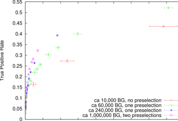
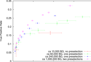
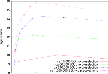
In Figure 1 the receiver operation characteristic (ROC) curves for using the four different training sets are shown (the plots are done using the test set). The ROC curve is defined as a plot of the true positive rate (or signal efficiency) versus the false positive rate (or background efficiency). We find that those classifier models corresponding to the training sets with larger background give superior results with respect to those where a training set with lower background has been used. This is especially evident in a zoom in Figure 2. Here, as almost everywhere else, we see that for a false positive rate of around $5\cdot 10^{-5}$ the classifier model corresponding to the largest background in the training sample is the best. From Figure 3 we see that this region in false positive rate is where the highest significance is. Thus this is an important working point.

data set	ca # BG	# sig.	# presel.
test	$6.5\cdot 10^{6}$	1827	–
training small	10,000	1851	0
training mid	60,000	1851	1
training larger	240,000	1851	1
training largest	1,000,000	1851	2

Table 3: The $D^{0}$ training and testing data sets. The second column contains the number of background candidates, the third column contains the number of signal candidates and the last column gives the number of preselections used.

Figure 1: ROC curve, i.e., true positive rate (signal efficiency) versus false positive rate (background efficiency), for using the different training samples. Mind that in this representation a curve being more to the upper left is better.

Figure 2: As Figure 1, but zoomed in.

Figure 3: Significance versus false positive rate for the $D^{0}$ selections using the different training samples.

Figure 4: The $D^{0}$ mass plot after a cuts based selection using the same variables.

Figure 5: The mass plot after our multivariate method, cost parameter set in a way to get the same signal yield as the cuts based analysis for comparison reasons.

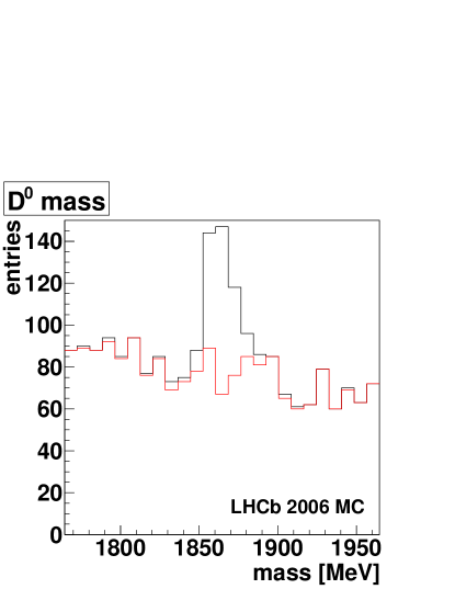
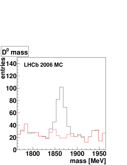
Figures 5 and 5 compare the mass plots of a cuts based $D^{0}$ selection using the same variables, and this multivariate method where the cost has been chosen to get the same signal yield as in the cuts based scheme. This was done for comparison reasons and we see that for the same signal yield the background is reduced drastically.

3 Forest cover type data

Is this behavior special to our data set or does it also appear on other kinds of data? From a data mining data set repository [Aha], we choose the data set called forest cover type (see also [BD99]). It is about predicting forest cover type from cartographic variables. The observations (30 $\times$ 30 meter cells) are wilderness areas with minimal human-caused disturbances as determined by the US Forest Service (USFS) in the Roosevelt National Forest of northern Colorado. The 54 variables include 10 integer variables, like elevation in feet, slope in degrees and vertical distance to nearest surface water. The rest of the variables are of categoric type indicating the wilderness and soil type. The classes to predict are seven cover types, like Spruce/Fir, Lodgepole Pine or Ponderosa Pine. We use the 10 integer variables only and use class 4 (Cottonwood/Willow) as “signal”, the rest as “background” to get an imbalanced data set. Splitting up the data set into test and training data, we have about 290,000 background instances and 1365 signal instances in the test set. For training about 240,000 background and 1382 signal instances are left. Again we use different training sets with the same number of signal (1382) but increasing number of background, namely 10,000, 60,000, 240,000 and 5 $\times$ 240,000, where in the last case we use a method to artificially replicate the background instances as described below. Also the number of preselections increases with the number of background instances in the training. We use no preselection in the case of 10,000 background instances, one preselection in the cases of 60,000 and 240,000 background instances and two preselections for the larges training sample. In this larges training sample we use additional artificial background data obtained by four times randomization of existing background instances using the SMOTE algorithm [CBHK02]. This was done to see if we can improve the result in spite of the fact that no more background events have been available.

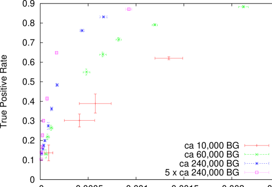
In Figure 7 we present the corresponding ROC curves. Again we see the same effect as for the $D^{0}$ data. In addition we see that adding artificial background data also improves the result.

Figure 6: The ROC curve for using the different training samples for the cover type data set.

Figure 7: The red ROC curve is plotted using no bagging, i.e., each point has been done using the same training sample. For the green curve, for each point the training set has been re-sampled, i.e., using one bagging iteration including a change in the random seed for each point in ROC space. The blue curve shows the effect of many (10) bagging iterations.

4 How to compare ROC curves with scatter

We have a different classifier model for each point in ROC space. But these classifier models depend not only on the training sample choice, but they also depend on random choices in bagging and in RIPPER during the training. Thus the pure ROC curves look noisy. So we need a way to find the expectation curve (i.e., average many) and a measure for the scatter (i.e., error bars).

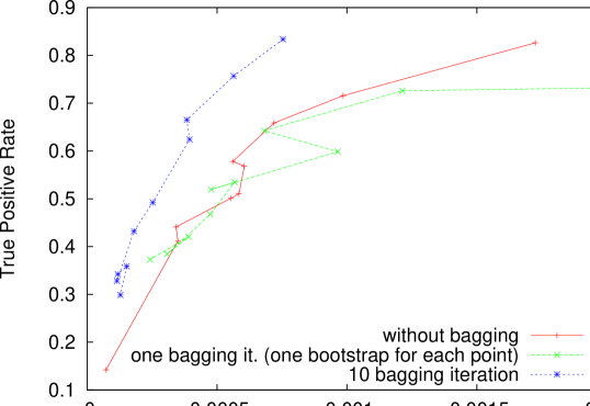
In Figure 7, the red curve uses the same sample for training for all points, for the green curve the training set has been re-sampled for each point. The less noisy curve (red) hides its scatter, i.e., its dependence on the training set. The same is true for ordinary ROC curves using a cut on a discriminant. The more noisy curve (green) tells us something about this scatter. As it should be, bagging reduces this scatter by using many bagging iterations (blue curve).

There are different methods for averaging ROC curves and to get error bars discussed in literature (see, e.g., [PFK98, PF01, DH04, MP04, MPR05a, MPR05b]). But none (that we could find) takes into account the scatter due to the training set. In our method we start by doing each main selection 10 times with different random seeds. Then we take the mean false positive rate (FPR) and true positive rate (TPR) as the point in ROC space. This is similar to using 10 cross-validation samples used in literature. But now we take the standard deviations as errors in FPR and TPF. The result is what is shown in the plots in Figures 1, 2 and 7. What is the distribution like?

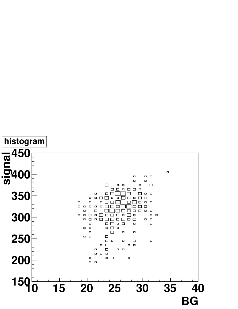
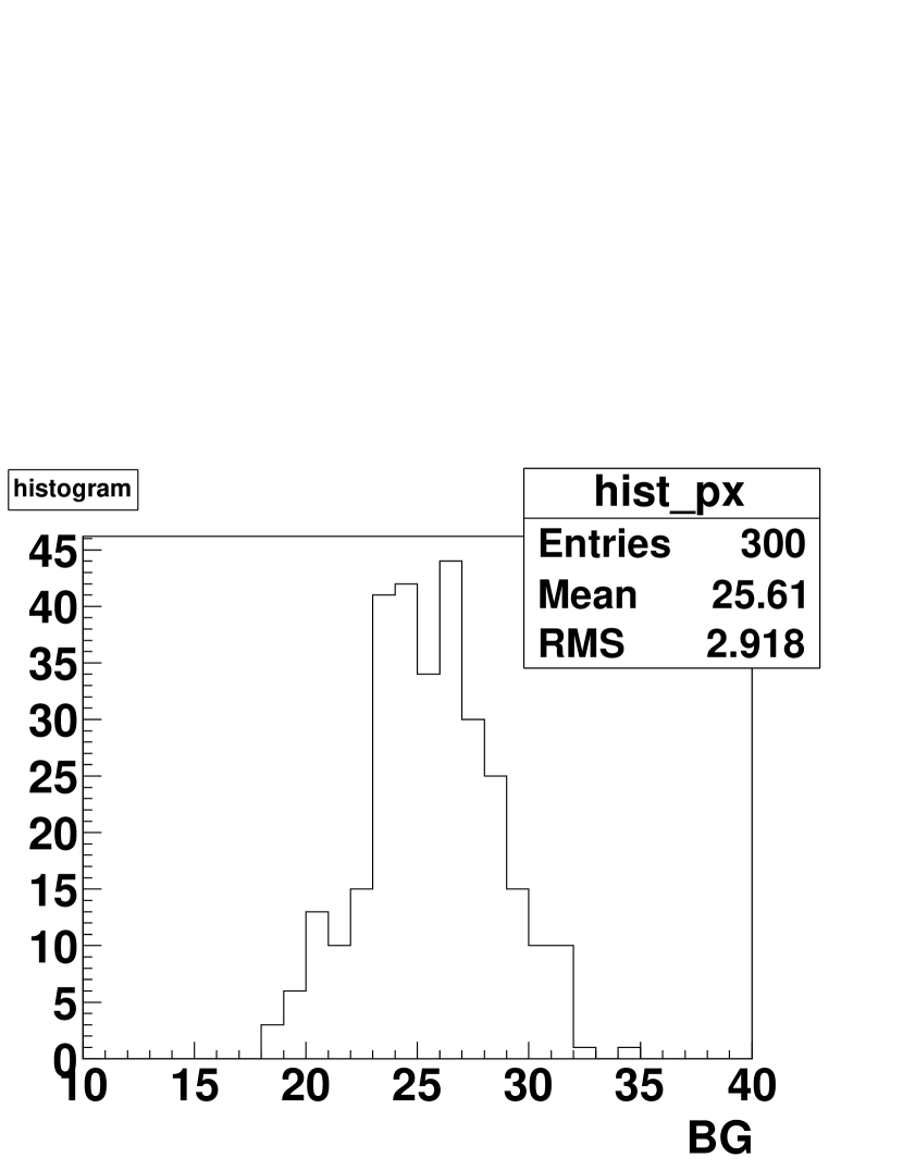
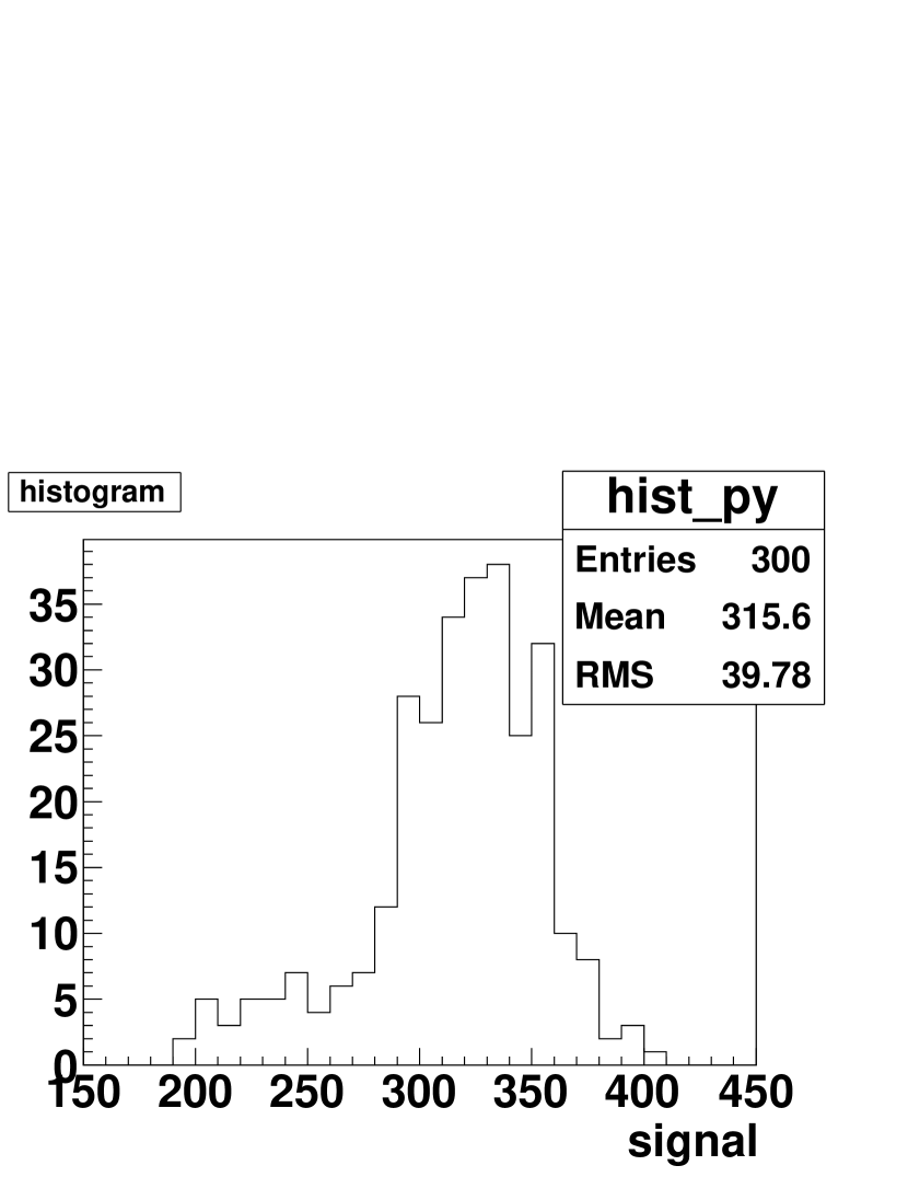
To find this out, we are using 300 samples of the same cost but different random seeds – with no averaging. This distribution in number of signal versus number of background candidates is shown in Figure 8 including the projections onto the background and signal axis respectively. The distributions are asymmetric and have tails, thus the standard deviation cannot be associated with a well defined confidence level. Nevertheless if we calculate the 68 % confidence level intervals for the background and the signal histograms in Figure 8, we get [23, 28] and [282, 351] respectively. This, possibly by pure coincidence, is very close to what we get as the one standard deviation interval from the mean and the RMS, i.e., [22.7, 28.5] for background and [276, 356] for signal respectively.

Figure 8: Shown on the left is a scatter plot (number of signal versus number of background) of 300 points using the same cost but different random seeds. In the middle its projection on the background axis is shown and on the right the projection on the signal axis.

5 Conclusion and Outlook

For extremely imbalanced data sets we have seen that more background in the training set is better for the LHCb $D^{0}$ selection as well as the forest cover type data set – in an important region of false positive rate. One or two preselections with less background helps reducing the data to handle large training sets. Even using extra artificial background instances helps.

For ROC curve errors, we have presented a method which seems reasonable and practical but the error-bars cannot be interpreted as a confidence level.

More sophisticated ways to reduce the data size without loosing classification quality have also been investigated by the authors [BGS]. Future work will include to search for better ways to average ROC curves and to produce error bars. In addition we want to try different classifiers (e.g., decision trees) to see if the behavior is a general one and not a special feature of the RIPPER algorithm. Finally we want to try this method on rare decays.