Abstract

We investigate the critical properties of the two-dimensional $Z(5)$ vector model. For this purpose, we propose a new cluster algorithm, valid for $Z(N)$ models with odd values of $N$. The two-dimensional $Z(5)$ vector model is conjectured to exhibit two phase transitions with a massless intermediate phase. We locate the position of the critical points and study the critical behavior across both phase transitions in details. In particular, we determine various critical indices and compare the results with analytical predictions.

  e-mail addresses:

^∗oleg@bitp.kiev.ua, ^∗∗cortese,fiore,papa@cs.infn.it, ^∗∗∗gravina@ucy.ac.cy

1 Introduction

The Berezinskii-Kosterlitz-Thouless (BKT) phase transition is known to take place in a variety of two-dimensional ($2D$) systems: certain spin models, two-dimensional Coulomb gas, sine-Gordon model, Solid-on-Solid model, etc., the most popular and elaborated case being the two-dimensional $XY$ model [1, 2, 3]. There are several indications that this type of phase transition is not a rare phenomenon in gauge models at finite temperature: one can argue that in some three-dimensional lattice gauge models the deconfinement phase transition is of BKT type as well. Here we are going to study an example of lattice spin model where this type of transition exhibits itself, namely the $2D$ $Z(N)$ spin model, also known as vector Potts model.

Consider a $2D$ lattice $\Lambda=L^{2}$ with linear extension $L$ and impose periodic boundary conditions on spin fields in both directions. The partition function of the model can be written as

$$Z(\Lambda,\beta)=\left[\prod_{x\in\Lambda}\frac{1}{N}\sum_{s(x)=0}^{N-1}\right]\left[\prod_{x\in\Lambda}\prod_{n=1,2}Q\left(s(x)-s(x+e_{n})\right)\right]\;.$$ (1)

In the standard formulation the most general $Z(N)$-invariant Boltzmann weight with $N-1$ different couplings is

$$Q(s)\ =\ \exp\left[\sum_{k=1}^{N-1}\beta_{k}\cos\frac{2\pi k}{N}s\right]\ .$$ (2)

In the Villain formulation the Boltzmann weight reads instead

$$Q(s)\ =\ \sum_{m=-\infty}^{\infty}\exp\left[-\frac{1}{2}\beta\left(\frac{2\pi}{N}s+2\pi m\right)^{2}\right]\ .$$ (3)

Some details of the critical behavior of $2D$ $Z(N)$ spin models are well known – see the review in Ref. [4]. The $Z(N)$ spin model in the Villain formulation (3) has been studied analytically in Refs. [5, 6, 7, 8, 9]. It was shown that the model has at least two phase transitions when $N\geq 5$. The intermediate phase is a massless phase with power-like decay of the correlation function. The critical index $\eta$ has been estimated both from the renormalization group (RG) approach of the Kosterlitz-Thouless type and from the weak-coupling series for the susceptibility. It turns out that $\eta(\beta^{(1)}_{\rm c})=1/4$ at the transition point from the strong coupling (high-temperature) phase to the massless phase, i.e. the behavior is similar to that of the $XY$ model. At the transition point $\beta^{(2)}_{\rm c}$ from the massless phase to the ordered low-temperature phase one has $\eta(\beta^{(2)}_{\rm c})=4/N^{2}$. A rigorous proof that the BKT phase transition does take place, and so that the massless phase exists, has been constructed in Ref. [10] for both Villain and standard formulations (with one non-vanishing coupling $\beta_{1}$). Monte Carlo simulations of the standard version with $N=6,8,12$ were performed in Ref. [11]. Results for the critical index $\eta$ agree well with the analytical predictions obtained from the Villain formulation of the model.

In this paper we thoroughly investigate the case $N=5$, the lowest number where the BKT transition is expected. Precisely, we concentrate on the standard formulation (2) with one non-zero coupling $\beta_{1}$. The motivation of our study is three-fold:

1. to compute critical indices at the transition points, which could serve as checking point of universality;

2. to shed light on the discrepancy in the literature concerning the $Z(5)$ model;

3. to develop and test a new version of Monte Carlo cluster algorithm valid for odd values of $N$.

The first motivation is related to the study of the finite-temperature transitions in $3D$ $Z(N)$ and $SU(N)$ lattice gauge theory (LGT). It is expected that in $3D$ $Z(N)$ LGT a deconfinement phase transition takes place at finite temperature. There is no precise statement about the order of the phase transition, but presumably it is of the BKT type if $N>4$. If it is the case, the Svetitsky-Yaffe conjecture [12] implies that the $3D$ $Z(N)$ LGT is in the universality class of $2D$ vector Potts model. Moreover, it can be proven that, in the strong coupling region with respect to the spatial coupling, the $3D$ $Z(N)$ LGT reduces to a $2D$ $Z(N)$ model with the general Boltzmann weight (2), and such that $\beta_{1}=\beta_{4}\gg\beta_{2}=\beta_{3}$, for $N=5$. Here, $\beta_{k}$ are effective couplings which depend on the gauge coupling and the temporal extension $N_{t}$. Thus, our $Z(5)$ model represents a good approximation to $3D$ $Z(5)$ LGT in this region.

Next, let $W(x)\in SU(N)$ and consider the following effective action in $2D$

$$S_{\rm eff}\ =\ \sum_{x,n}\ {\rm Tr}W(x){\rm Tr}W^{\dagger}(x+e_{n})+{\rm c.c.}\;.$$ (4)

The effective action (4) can be regarded as the simplest effective model for the Polyakov loop which can be derived in the strong coupling region of $3D$ $SU(N)$ LGT at finite temperature. It possesses $Z(N)$ global symmetry and thus may well exhibit the BKT transitions which belong to the universality class of the corresponding vector Potts model. Therefore, our investigation here can be viewed as a preliminary step in studying deconfinement phase transition in $3D$ $Z(N)$ and $SU(N)$ LGTs.

The second motivation reflects the fact that many features of the critical behavior of the $Z(5)$ model are not reliably established. Moreover, there are certain discrepancies even in determining the nature of the phase transition, i.e. whether the phase transition is of BKT type or not.

Let us briefly summarize the present state of affairs.

• The rigorous proof of the massless phase existence in $2D$ $Z(N)$ models utilizes methods which do not allow to establish the exact value of $N$ above which the BKT phase transition exists [10].

• Reliable analytical calculations can only be performed with the Villain formulation (3); the RG study of Ref. [5] predicts that the massless phase exists for all $N>4$.

• Some information on the phase structure of the general $Z(N)$ spin models can be obtained through the duality transformations (see, e.g. [13]). These transformations cannot be used to establish the position of the critical points in the $Z(5)$ model [14]. However, duality transformations relate the two critical points and thus can be used to verify the accuracy of numerical data. Moreover, one can predict an approximate phase diagram and argue that the massless phase and the BKT transition exist for $N=5$ in a certain region of the parameter space [15, 16]. Important in this context is the rigorous proof of the existence of the massless phase, constructed in Ref. [15] for the generalized Villain formulation. This generalized formulation contains the vector Potts model defined in (2) with one non-zero coupling $\beta_{1}$ as a particular case.

  For completeness we mention that in Refs. [17] it was suggested that there is only one first order phase transition in $Z(5)$ model. This, however, contradicts the rigorous results of [15].

• An analytical prediction for the critical index $\eta$ has been obtained for the Villain formulation in Ref. [5]: $\eta(\beta^{(1)}_{\rm c})=1/4$ and $\eta(\beta^{(2)}_{\rm c})=0.16$ (for $N=5$). The situation remains unclear for the index $\nu$ which governs the behavior of the correlation length. Normally, the value of $\nu$ can be estimated from the solution of the RG equations like in the $XY$ model [3]. The analytical solution of the system of RG equations for $Z(N)$ vector models is unknown (see Ref. [5]). Therefore, strictly speaking, there are no strong theoretical arguments indicating that $\nu=1/2$, similarly to the $XY$ model. Moreover, the strong coupling expansion of the $Z(5)$ model combined with Padé approximants predicts that $\nu\approx 0.22$ [5].

• Monte Carlo simulations of the $Z(N)$ model have been performed in Refs. [11, 18, 19, 20]. Results of Ref. [18], though obtained on rather small lattices, indicate that the BKT transition takes place in models with $N\geq 8$. This contradicts the results of [11, 20] which well agree with the BKT behavior for $N=6$.

  However, most recent simulations of the helicity modulus in the $Z(5)$ model at $\beta^{(1)}_{\rm c}$ do not agree with what is expected at the BKT transition [19]. Namely, at the critical point the helicity modulus is expected to jump discontinuously to zero, and the jump is observed for $Z(6)$ model, while in $Z(5)$ the helicity modulus stays small but non-vanishing in the high-temperature region $\beta<\beta^{(1)}_{\rm c}$.

Still, it remains unclear how this behavior of the helicity modulus influences other features of the BKT transition. The key feature of the massless BKT phase in $Z(N)$ models is the enhancement of the discrete symmetry of the Hamiltonian: the symmetry of the ground state in the intermediate phase is rather $U(1)$ than $Z(N)$ [10]. This can be seen in a characteristic distribution of the complex magnetization, in the power-like decay of the correlation functions in the massless phase, in the vanishing of the beta-function, etc.. Also, on the basis of the universality one could conjecture that the critical indices in the $Z(5)$ model are the same both in the standard and Villain formulations. We are not aware of any numerical calculations of these quantities in $Z(5)$. Here we would like to fill this gap by computing various quantities and extracting critical indices at both transitions. Among the main quantities calculated in this paper there are Binder cumulants. As RG invariant quantities, Binder cumulants are very useful in locating the critical couplings and determining the nature of the phase transition. Indeed, the computation of Binder cumulants proved to be very efficient in studying BKT transitions in a variety of models, like the $XY$ model, the discrete Gaussian model and the SOS model [21]. We therefore believe that these cumulants are of great value also in the investigation of phase transitions in $2D$ $Z(N)$ models. Preliminary results of our study have been presented in Ref. [22].

The paper is organized as follows: in Section 2 we describe the set-up of the Monte Carlo simulation and the newly developed cluster algorithm; in Section 3 we introduce the observables adopted in this work and study the transition from the high-temperature to the massless phase; in Section 4 we move on to consider the transition from the massless to the low-temperature ordered phase; finally in Section 5 we draw our conclusions. In the Appendix we check the consistency of our determination of the critical couplings with the duality transformations.

2 Algorithm and numerical set-up

In this work we concentrate our attention to the model defined by Eqs. (1) and (2), with only one non-zero coupling, $\beta_{1}\equiv\beta$ . This model is known in the literature also as $N$-state ferromagnetic clock model and is a discrete version of the continuous $XY$ (plane rotator) model. It consists of 2D planar spins restricted to $N$ evenly spaced directions, with spin interaction energy proportional to their scalar product.

The Hamiltonian of the model is

$$H=-\beta\sum_{\langle ij\rangle}\cos\left(\frac{2\pi}{N}(s_{i}-s_{j})\right)\;,\;\;\;\;\;s_{i}=0,1,\ldots,N-1\;,$$ (5)

with summation taken over nearest-neighbor sites. For $N=2$ this is the Ising model, whereas in the $N\rightarrow\infty$ limit we get the $XY$ model.

Here we develop a new algorithm, valid for odd $N$, by which an accurate numerical study of the model can be performed for $N=5$, i.e. the smallest $N$ value for which the phase structure described in the Introduction holds.

Here are the steps of our cluster algorithm for the update of a spin configuration $\{s_{i}\}$:

• choose randomly $n$ in the set $\{0,1,2,\ldots,N-1\}$

• build a cluster configuration according to the following probability of bond activation between neighboring sites $ij$

  $$p_{ij}=\left\{\begin{array}[]{cl}1-\exp(-2\beta\ \alpha_{i}\alpha_{j})&{\rm if}\;\alpha_{i}\alpha_{j}>0\\ 0&{\rm otherwise}\\ \end{array}\right.\;,\;\;\;\;{\rm with}\;\;\alpha_{k}\equiv\sin\left(\frac{2\pi}{N}(s_{k}-n)\right)$$

• “flip” each cluster, with probability 1/2, by replacing all its spins according to the transformation

  $$s_{i}\rightarrow{\rm mod}(-s_{i}+2n+N,N)\;,$$

  which amounts to replacing each spin $s_{i}$ in a cluster by the spin $s_{j}$ for which $\alpha_{j}=-\alpha_{i}$; equivalently, if the spins are mapped into the $N$ roots of unity in the complex plane, the above replacement means flipping the component of each spin transverse to the direction identified by $n$.

It is easy to prove that this cluster algorithm fulfills the detailed balance.

We have tested the efficiency of the cluster algorithm against the standard heat-bath algorithm. On a lattice with $L=64$ we simulated the model with $N=5$ and determined the autocorrelation time $\tau$ of three observables: the energy, defined in Eq. (5), the magnetization $M_{L}$ and the population $S_{L}$, to be defined below. We considered three $\beta$ values (0.80, 1.10 and 1.50) lying, respectively, in the high-temperature, massless and low-temperature phase of the model. Results are summarized in Table 1, whose last two columns give also the number of sweeps needed to reach thermal equilibrium and the computer time to collect a 50k statistics.

Table 1: Cluster versus heat-bath in $Z(5)$ on a $64^{2}$ lattice at three values of $\beta$: autocorrelation time $\tau$ for three observables (energy, magnetization $M_{L}$ and population $S_{L}$), number of thermalization sweeps and computer time for 50k updates.

		Energy	$M_{L}$	$S_{L}$	Thermalization	Time
	cluster	5.135(82)	1.528(38)	1.494(39)	$\sim 10$	46.69 s
$\beta=0.80$	heat-bath	5.43(33)	12.83(27)	12.65(28)	$\sim 100$	1290 s
	cluster	7.36(11)	5.56(10)	7.18(11)	$\sim 10$	45.14 s
$\beta=1.10$	heat-bath	10.11(48)	48.3(4.8)	60.6(6.1)	$\sim 1000$	1194 s
	cluster	8.97(17)	8.71(17)	8.84(17)	$\sim 100$	42.60 s
$\beta=1.50$	heat-bath	2.38(12)	3.73(15)	3.78(13)	$\sim 6500$	1064 s

At $\beta$=0.80 and 1.10 the autocorrelation time in the cluster algorithm is lower than in the heat-bath for the energy and much lower for magnetization and population. At $\beta=1.50$, deep in the low-temperature ordered phase, $\tau$ is systematically higher in the cluster than in the heat-bath. This is a consequence of the lowering of the bond activation probability for increasing $\beta$. This drawback, however, is compensated by the higher simulation speed, with respect to the heat-bath algorithm. Moreover since the two transitions in the $2D$ $Z(5)$ model are rather close (see below), there is no doubt that the cluster algorithm is strongly preferable.

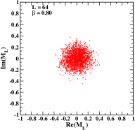
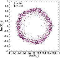
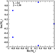
Figure 1: (Color online) Scatter plot of the complex magnetization $M_{L}$ at $\beta=0.80,1.10,1.50$ in $Z(5)$ on a $64^{2}$ lattice.

The improvement brought along by the cluster algorithm becomes more visible when the dynamical critical exponent $z$ is considered, defined as $\tau\sim\xi^{z}$, where $\xi$ is the correlation length. We have evaluated $z$ in the $2D$ $Z(5)$ model on lattices with $L=16,32,64,128,256,384,512$ at both transition points, using the autocorrelation time of the magnetization $M_{L}$. Since at both points the correlation length diverges, the expected scaling law becomes $\tau\sim L^{z}$. We got in all cases that $\tau$ keeps almost constant at $\approx 7$, thus implying $z\simeq 0$, i.e. no critical slowing down.

The three phases exhibited by the $2D$ $Z(5)$ spin model can be characterized by means of two observables: the complex magnetization $M_{L}$ and the population $S_{L}$.

The complex magnetization is given by

$$M_{L}=\frac{1}{L^{2}}\sum_{i}\exp\left(i\frac{2\pi}{N}s_{i}\right)\equiv|M_{L}|e^{i\psi}\;.$$ (6)

In Fig. 1 we show the scatter plot of $M_{L}$ on a lattice with $L=64$ in $Z(5)$ at three values of $\beta$, each representative of a different phase: $\beta=0.80$ (high-temperature, disordered phase), $\beta=1.10$ (BKT massless phase) and $\beta=1.50$ (low-temperature, ordered phase). As we can see we pass from a uniform distribution (low $\beta$) to a ring distribution (intermediate $\beta$) and finally to five isolated spots (high $\beta$).

The naive average of the complex magnetization gives constantly zero, therefore $M_{L}$ is not an order parameter. An observable to detect the transition from one phase to the other is instead the absolute value $|M_{L}|$ of the complex magnetization. In Fig. 2 we show the behavior of $|M_{L}|$ and of its susceptibility,

$$\chi^{(M)}_{L}=L^{2}(\langle|M_{L}|^{2}\rangle-\langle|M_{L}|\rangle^{2})\;,$$ (7)

in $Z(5)$ on lattices with $L$ ranging from 16 to 1024 over a wide interval of $\beta$ values. On each lattice the susceptibility $\chi^{(M)}_{L}$ clearly exhibits two peaks, the first of them, more pronounced than the other, identifies the pseudocritical coupling $\beta^{(1)}_{\rm pc}(L)$ at which the transition from the disordered to the massless phase occurs, whereas the second corresponds to the pseudocritical coupling $\beta^{(2)}_{\rm pc}(L)$ of the transition from the massless to the ordered phase. It is evident from Fig. 2 that $|M_{L}|$ is particularly sensitive to the first transition, thus making this observable the best candidate for studying its properties.

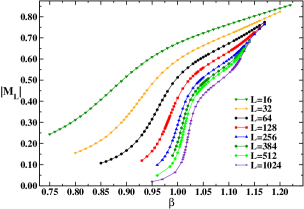
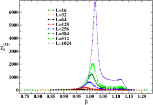
Figure 2: (Color online) Behavior of $|M_{L}|$ (left) and of its susceptibility $\chi^{(M)}_{L}$ (right) versus $\beta$ in $Z(5)$ on lattices with $L$ ranging from 16 to 1024.

As order parameter to better detect the second transition, i.e. that from the massless to the ordered phase, we chose instead the population $S_{L}$, defined as

$$S_{L}=\frac{N}{N-1}\left[\frac{\max_{i=0,N-1}(n_{i})}{L^{2}}-\frac{1}{N}\right]\;,$$ (8)

where $n_{i}$ represents the number of spins of a given configuration which are in the state $s_{i}$. In a phase in which there is not a preferred spin direction in the system (disorder), we have $n_{i}\sim L^{2}/N$ for each index $i$, therefore $S_{L}\sim 0$. Otherwise, in a phase in which there is a preferred spin direction (order), we have $n_{i}\sim L^{2}$ for a given index $i$, therefore $S_{L}\sim 1$. In Fig. 3 we show the behavior of $S_{L}$ and of its susceptibility

$$\chi^{(S)}_{L}=L^{2}(\langle S_{L}^{2}\rangle-\langle S_{L}\rangle^{2})\;,$$ (9)

in $Z(5)$ on lattices with $L$ ranging from 16 to 1024 over a wide interval of $\beta$ values. Again the peaks signalling the two transitions are clearly visible and their positions agree with Fig. 2, but now the second one is more pronounced.

Other observables which have been used in this work are the following:

• the real part of the “rotated” magnetization, $M_{R}=|M_{L}|\cos(N\psi)$,

• the order parameter introduced in Ref. [20], $m_{\psi}=\cos(N\psi)$,

where $\psi$ is the phase of the complex magnetization defined in Eq. (6).

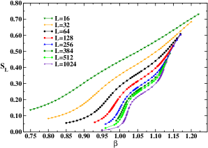
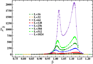
Figure 3: (Color online) Behavior of $S_{L}$ (left) and of its susceptibility $\chi^{(S)}_{L}$ (right) versus $\beta$ in $Z(5)$ on lattices with $L$ ranging from 16 to 1024.

In the next two Sections we will study separately the two transitions of $2D$ $Z(5)$ and determine some of the related critical indices. For all observables considered in this work we collected typically 100k measurements, on configurations separated by 10 updating sweeps. For each new run the first 10k configurations were discarded to ensure thermalization. Data analysis was performed by the jackknife method over bins at different blocking levels.

3 The transition from the high-temperature to the massless phase

The first inflection point in the plot of the magnetization $|M_{L}|$ and the first peak in the plot of the susceptibility $\chi_{L}^{(M)}$ (see Fig. 2) indicate the transition from the disordered to the massless phase. The couplings where this transition occurs (denoted as the pseudocritical couplings $\beta_{\rm pc}^{(1)}(L)$) have been determined by a Lorentzian interpolation around the peak of the susceptibility $\chi_{L}^{(M)}$. Their values are summarized in the second column of Table 2. We observe that, when the lattice size $L$ grows, $\beta_{\rm pc}^{(1)}(L)$ increases towards the infinite volume critical coupling $\beta^{(1)}_{\rm c}$ and that the susceptibility $\chi^{(M)}_{L}$ goes to zero less rapidly for $\beta>\beta^{(1)}_{\rm pc}$, as expected in the BKT scenario.

Table 2: Values of $\beta^{(1)}_{\rm pc}$ in $Z(5)$ on $L^{2}$ lattices. The last two columns give the susceptibility $\chi^{(M)}_{L}$ and the magnetization $|M_{L}|$ at the infinite volume coupling constant $\beta^{(1)}_{\rm c}$=1.0510.

$L$	$\beta^{(1)}_{\rm pc}$	$\chi^{(M)}_{L}(\beta^{(1)}_{\rm c})$	$|M_{L}|(\beta^{(1)}_{\rm c})$
16	0.8523(20)	-	-
32	0.91429(90)	-	-
64	0.95373(40)	-	-
128	0.98054(30)	-	-
256	0.99838(20)	-	-
384	1.00621(10)	187.9(1.2)	0.48929(13)
512	1.01112(20)	311.5(2.0)	0.47181(13)
640	-	458.6(3.4)	0.45918(11)
768	-	631.3(4.2)	0.44863(11)
896	-	824.4(5.2)	0.44004(11)
1024	1.01991(10)	1040.0(6.9)	0.43277(11)

In order to apply the finite size scaling (FSS) program, the location of the infinite volume critical coupling $\beta^{(1)}_{c}$ is needed. In Refs. [23, 24] this was done by extrapolating the pseudocritical couplings to the infinite volume limit, according to a suitable scaling law. First order transition is ruled out by data in Table 2. Second order transition, though not incompatible with data in Table 2, is to be excluded, due to the vanishing of the long distance correlations combined with the clusterization property (we will come back to this point in the last Section). Therefore, we assume that the transition is of BKT type and adopt the scaling law dictated by the essential scaling of the BKT transition, i.e. $\xi\sim e^{bt^{-\nu}}$, which reads

$$\beta^{(1)}_{\rm pc}=\beta^{(1)}_{\rm c}+\frac{A}{(\ln L+B)^{\frac{1}{\nu}}}\quad.$$ (10)

The index $\nu$ characterizes the universality class of the system. For example, $\nu=1/2$ holds for the 2$D$ $XY$ universality class.

Unfortunately, 4-parameter fits of the data for $\beta^{(1)}_{\rm pc}(L)$ give very unstable results for the parameters. This led us to move to 3-parameter fits of the data, with $\nu$ fixed at 1/2. We found, as best fit with the MINUIT optimization code,

$$\beta^{(1)}_{\rm c}=1.0602(20)\;,\;\;A_{1}=-2.09(20)\;,\;\;B_{1}=0.27(18)\;,\;\;\chi^{2}/{\rm d.o.f.}=0.48\;,\;\;L_{\rm min}=64\;.$$

We observe that $\beta^{(1)}_{\rm c}$ is rather far from the value of $\beta^{(1)}_{\rm pc}$ on the largest available lattice, thus casting some doubts on the reliability of the extrapolation to the thermodynamic limit. For this reason, we turned to an independent method for the determination of $\beta^{(1)}_{\rm c}$, based on the use of Binder cumulants.

In particular, we considered the reduced 4-th order Binder cumulant $U^{(M)}_{L}$ defined as

$$U^{(M)}_{L}=1-\frac{\langle|M_{L}|^{4}\rangle}{3\langle|M_{L}|^{2}\rangle^{2}}\;,$$ (11)

and the cumulant $B_{4}^{(M_{R})}$ defined as

$$B_{4}^{(M_{R})}=\frac{\langle|M_{R}-\langle M_{R}\rangle|^{4}\rangle}{\langle|M_{R}-\langle M_{R}\rangle|^{2}\rangle^{2}}\;.$$ (12)

Plots of the various Binder cumulants versus $\beta$ show that data obtained on different lattice volumes align on curves that cross in two points, corresponding to the two transitions (see Figs. 4 and 5). We used also the reduced 4-th order Binder cumulant of the action which showed no crossing points nor volume-dependent dips, thus confirming the absence of first order phase transitions.

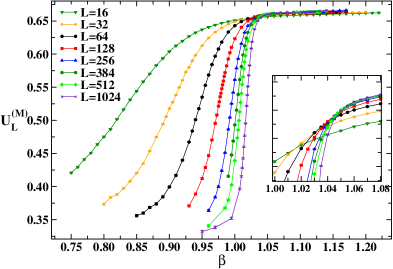
Figure 4: (Color online) Reduced 4-th order Binder cumulant $U^{(M)}_{L}$ versus $\beta$ on lattices with $L$ ranging from 16 to 1024.

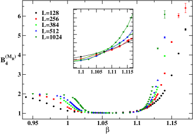
Figure 5: (Color online) Binder cumulant $B_{4}^{(M_{R})}$ versus $\beta$ on lattices with $L$ ranging from 128 to 1024.

We determined the crossing point by plotting the Binder cumulants versus $(\beta-\beta_{\rm c})(\ln L)^{1/\nu}$, with $\nu$ fixed at 1/2, and by looking for the optimal overlap of data from different lattices, by the $\chi^{2}$ method (see Fig. 6 for an example of this kind of plots). As a result of this analysis we arrived at the following estimate: $\beta^{(1)}_{\rm c}=1.0510(10)$. We observe that $\beta^{(1)}_{\rm c}$ is not compatible with the infinite volume extrapolation of the corresponding pseudocritical couplings, thus confirming our previous worries about the safety of the infinite volume extrapolation of $\beta^{(1)}_{\rm pc}$. It should be noted, however, that a fit to $\beta^{(1)}_{\rm pc}(L)$ with the law (10) and with $\beta^{(1)}_{\rm c}$ fixed at 1.0510 and $\nu$ fixed at 1/2 gives a good $\chi^{2}$/d.o.f., if only the three largest volumes are considered in the fit.

We have also tested the strong coupling prediction of Ref. [5] suggesting $\nu=0.22$. In particular, we have plotted the Binder cumulant $U^{(M)}_{L}$ versus $(\beta-\beta_{\rm c})(\ln L)^{1/\nu}$, with $\nu$ fixed now at the candidate value 0.22. We have seen that, varying $\beta_{\rm c}$ on a wide interval, the overlap among curves from different lattices is always rather poor.

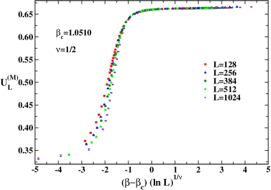
Figure 6: (Color online) Reduced 4-th order Binder cumulant $U^{(M)}_{L}$ versus $(\beta-\beta_{\rm c})(\ln L)^{1/\nu}$, for $\beta_{\rm c}=1.0510$ and $\nu=1/2$ on lattices with $L$ ranging from 128 to 1024.

Table 3: Results of the fit to the data of $|M_{L}|(\beta^{(1)}_{\rm c})$ with the scaling law (13) on $L^{2}$ lattices with $L\geq L_{\rm min}$.

$L_{\rm min}$	$A$	$\beta/\nu$	$\chi^{2}$/d.o.f.
384	1.0299(21)	0.12508(32)	1.3
512	1.0294(32)	0.12501(47)	1.7
640	1.0371(49)	0.12610(71)	0.40
768	1.0305(89)	0.1252(13)	0.021

Table 4: Results of the fit to the data of $\chi^{(M)}_{L}(\beta^{(1)}_{\rm c})$ with the scaling law (14) on $L^{2}$ lattices with $L\geq L_{\rm min}$.

$L_{\rm min}$	$A$	$\gamma/\nu$	$\chi^{2}$/d.o.f.
384	0.00586(30)	1.7438(80)	0.060
512	0.00602(48)	1.740(12)	0.018
640	0.00598(81)	1.741(20)	0.025
768	0.0062(14)	1.735(34)	0.0063

We are now in the position to extract other critical indices and check therefore the hyperscaling relation. According to the standard FSS theory, in a $L\times L$ lattice at criticality the equilibrium magnetization $|M_{L}|$ should obey the relation $|M_{L}|\sim L^{-\beta/\nu}$, for sufficiently large $L$ . We performed a fit to the data of $|M_{L}|(\beta^{(1)}_{\rm c})$ (reported in the last column of Table 2) on all lattices with size $L$ not smaller than a given $L_{\rm min}$ according to the scaling law

$$|M_{L}|=AL^{-\beta/\nu}$$ (13)

and summarized our results in Table 3.

The FSS behavior of the $\chi^{(M)}_{L}$ susceptibility defined in Eq. (7) is given by $\chi^{(M)}_{L}\sim L^{\gamma/\nu}$, where $\gamma/\nu=2-\eta$ and $\eta$ is the magnetic critical index. We performed a fit to the data of $\chi^{(M)}_{L}(\beta^{(1)}_{\rm c})$ (reported in the third column of Table 2) on all lattices with size $L$ not smaller than a given $L_{\rm min}$ according to the scaling law

$$\chi^{(M)}_{L}=AL^{\gamma/\nu}$$ (14)

and summarized our results in Table 4. As we can see, for all values of $L_{\rm min}$ considered, the value of the magnetic index  $\eta^{(1)}\equiv 2-\gamma/\nu$ is compatible with 1/4. Note also that the hyperscaling relation $\gamma/\nu+2\beta/\nu=d$, where $d$ is the dimension of the system, is always satisfied within the statistical error.

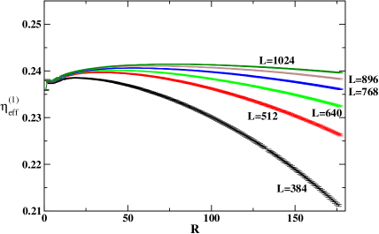
Figure 7: (Color online) $\eta^{(1)}_{\rm eff}$ versus $R$ at $\beta^{(1)}_{\rm c}=1.0510$ on lattices with $L=384,512,640,768,896,1024$.

An independent determination of the magnetic index $\eta$ can be achieved by the approach developed in Ref. [23]: an effective $\eta$ index is defined, through the spin-spin correlation function $\Gamma(R)$, according to

$$\eta^{(1)}_{\rm eff}(R)\equiv\frac{\ln[\Gamma(R)/\Gamma(R_{0})]}{\ln[R_{0}/R]}\quad,$$ (15)

with $R_{0}$ chosen equal to 10, as in Ref. [23]. This quantity is constructed in such a way that it exhibits a plateau in $R$ if the correlator obeys the law

$$\Gamma(R)\ \asymp\ \frac{1}{R^{\eta(T)}}\ ,$$ (16)

valid in the BKT phase, $\beta\geq\beta^{(1)}_{\rm c}$. In Fig. 7 we show the behavior of $\eta^{(1)}_{\rm eff}(R)$ at the infinite volume critical coupling $\beta^{(1)}_{\rm c}=1.0510$ on lattices with $L=384,512,640,768,896,1024$. It turns out that a plateau develops at small distances when $L$ increases and that the extension of this plateau gets larger with $L$, consistently with the fact that finite volume effects are becoming less important. The plateau value of $\eta^{(1)}_{\rm eff}$ can be estimated at about 0.24. We checked that this result is stable under variation of the parameter $R_{0}$. The discrepancy with the expected value of $1/4$ can be explained by the imperfect localization of the critical point and/or by the effect of logarithmic corrections [25, 26] that we were not able to include in our analysis.

Table 5: Values of $\beta^{(2)}_{\rm pc}$ in $Z(5)$ on $L^{2}$ lattices. The last two columns give the susceptibility $\chi^{(M_{R})}_{L}$ and the rotated magnetization $M_{R}$ at the infinite volume coupling constant $\beta^{(2)}_{\rm c}$=1.1048.

$L$	$\beta^{(2)}_{\rm pc}$	$\chi^{(M_{R})}_{L}(\beta^{(2)}_{\rm c})$	$M_{R}(\beta^{(2)}_{\rm c})$
16	1.1323(19)	-	-
32	1.1363(11)	-	-
64	1.13212(60)	-	-
128	1.12875(66)	-	-
256	1.12290(16)	-	-
384	1.12103(50)	47116(77)	0.1618(18)
512	1.11912(28)	80057(139)	0.1575(19)
640	-	120777(229)	0.1557(20)
768	-	169358(298)	0.1517(19)
896	-	224879(339)	0.1502(16)
1024	1.11596(38)	288151(532)	0.1473(18)

4 The transition from the massless to the low-temperature ordered phase

The second inflection point in the plot of the population $S_{L}$ and the second peak in the plot of the susceptibility $\chi_{L}^{(S)}$ (see Fig. 3) indicate the transition from the massless to the ordered phase. The couplings where this transition occurs (denoted as the pseudocritical couplings $\beta_{\rm pc}^{(2)}(L)$) have been determined by a Lorentzian interpolation around the peak of the susceptibility $\chi_{L}^{(S)}$. Their values are summarized in the second column of Table 5.

Available results in the literature [5, 11] suggest that the correlation length diverges according to essential scaling scenario when the critical point is approached from above. Our aim is to check the validity of this statement and then extract relevant indices characterizing the system at this transition. Again, first order transition is ruled out by data in Table 5 (and by the aforementioned analysis of the Binder cumulant of the action), while second order is not. We assume that a BKT transition is at work here and, therefore, that pseudocritical couplings scale with $L$ according to the law (10). As before, 4-parameter fits of the data for $\beta^{(2)}_{\rm pc}(L)$ are unstable and we moved to 3-parameter fits of the data, with $\nu$ fixed at 1/2, finding that the parameter $B_{2}$ turns out to be compatible with zero, so that, in fact, a 2-parameter fit works well:

$$\beta^{(2)}_{\rm c}=1.1042(12)\;,\;\;A_{2}=0.578(41)\;,\;\;B_{2}=0.\;,\;\;\chi^{2}/{\rm d.o.f.}=0.61\;,\;\;L_{\rm min}=128\;.$$

Now $\beta^{(2)}_{\rm c}$ is not far from the value of $\beta^{(2)}_{\rm pc}$ on the largest available lattice, thus supporting the reliability of the extrapolation to the thermodynamic limit.

Table 6: Results of the fit to the data of $\chi^{(M_{R})}_{L}(\beta^{(2)}_{\rm c})$ with the scaling law (14) on $L^{2}$ lattices with $L\geq L_{\rm min}$.

$L_{\rm min}$	$A$	$\gamma/\nu$	$\chi^{2}$/d.o.f.
384	0.799(11)	1.8459(21)	0.23
512	0.791(17)	1.8473(32)	0.19
640	0.784(28)	1.8487(53)	0.22
768	0.793(50)	1.8470(92)	0.39

Table 7: Results of the fit to the data of $M_{R}(\beta^{(2)}_{\rm c})$ with the scaling law (13) on $L^{2}$ lattices with $L\geq L_{\rm min}$.

$L_{\rm min}$	$A$	$\beta/\nu$	$\chi^{2}$/d.o.f.
384	0.281(26)	0.093(14)	0.15
512	0.288(41)	0.096(22)	0.18
640	0.322(77)	0.112(36)	0.12
768	0.30(12)	0.102(60)	0.19

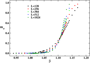
Figure 8: (Color online) Behavior of $m_{\psi}$ versus $\beta$ on lattices with $L$ ranging from 128 to 1024.

In order to localize the critical coupling $\beta_{\rm c}^{(2)}$, we looked for the crossing point at higher $\beta$ of the Binder cumulant $B_{4}^{(M_{R})}$ defined in Eq. (12) and repeated the analysis based on the optimal overlap of data points when they are plotted against $(\beta-\beta_{\rm c})(\ln L)^{1/\nu}$, with $\nu$ fixed at 1/2. The same procedure was carried on using also the observable $m_{\psi}$, which is itself an RG-invariant quantity and shares therefore the same properties of a Binder cumulant (see Fig. 8 for the behavior of $m_{\psi}$ versus $\beta$ on various lattices, which shows two crossing points, the one at higher $\beta$ corresponding to the transition from the massless to the ordered phase). This analysis led to the result $\beta^{(2)}_{\rm c}=1.1048(10)$, which agrees with the infinite volume extrapolation of the corresponding pseudocritical couplings.

We can now determine the ratios of critical indices $\beta/\nu$ and $\gamma/\nu$ as we did in the previous Section. It should be noted, however, that the population $S_{L}$ and its susceptibility are not suitable observables for this purpose, being defined in a non-local manner and, thus, not directly related to the two-point correlator. We use, instead, the rotated magnetization $M_{R}$ and its susceptibility $\chi^{(M_{R})}_{L}$ and compare their values at the infinite volume critical coupling $\beta^{(2)}_{\rm c}$ (see the last two columns of Table 5) with the scaling laws (13) and (14), respectively. Results for $\beta/\nu$ and $\gamma/\nu$ are summarized in Tables  6 and 7.

All the values for $\eta^{(2)}=2-\gamma/\nu$ given in Table 6 are in agreement with the prediction $4/N^{2}$, which gives 0.16 for $N=5$. The hyperscaling relation $\gamma/\nu+2\beta/\nu=d$ is always satisfied, within the statistical error.

The determination of the magnetic critical index based on the effective $\eta$ index defined in (15) is plagued, in this region of values of $\beta$, by a sizeable dependence on the choice of the arbitrary parameter $R_{0}$. The shape of the curves for $\eta_{\rm eff}(R)$ and the way they depend on $R_{0}$ suggest that here logarithmic corrections to the scaling could be at work. However, our data are not accurate enough to include them reliably in our fits.

We conclude this Section by presenting several examples of a posteriori check of consistency of our determinations for $\eta^{(1)}$ and $\eta^{(2)}$. The basic idea is to build plots in which we correlate two RG-invariant quantities and to check that sequences of data points, corresponding to different values of $\beta$, fall on a universal curve, irrespective of the lattice size $L$ [27, 28].

The first example is the plot of the rescaled susceptibility $\chi_{L}^{(M_{R})}L^{\eta-2}$ against the Binder cumulant $B_{4}^{(M_{R})}$. One can see from Fig. 9(a) that for $\eta=0.26\simeq\eta^{(1)}$ data points from different lattices fall on the same curve in the lower branch, corresponding to $\beta$ values in the region of the first transition; for $\eta=0.16\simeq\eta^{(2)}$, on the contrary, data points from different lattices fall on the same curve in the upper branch, corresponding to $\beta$ values in the region of the second transition (see Fig. 9(b)).

Another example is provided by the plot of the rescaled magnetization $M_{R}L^{\eta/2}$ against $m_{\psi}$. For $\eta=0.16\simeq\eta^{(2)}$, again data points from different lattices fall on the same curve (see Fig. 10).

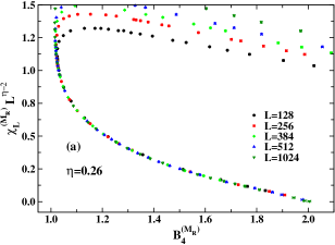
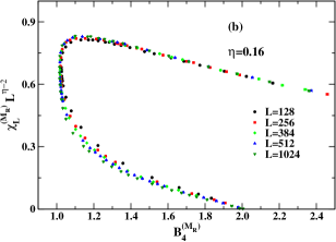
Figure 9: (Color online) Correlation between $\chi_{L}^{(M_{R})}L^{\eta-2}$ and the Binder cumulant $B_{4}^{(M_{R})}$ for (a) $\eta=0.26$ and (b) $\eta=0.16$ on lattices with $L$ ranging from 128 to 1024. For $\eta=0.26$ (a) data from different lattices tend to fall on a universal curve in the lower branch, corresponding to $\beta$ values in the region of the first transition. For $\eta=0.16$ (b) data from different lattices tend to fall on a universal curve in the upper branch, corresponding to $\beta$ values in the region of the second transition.

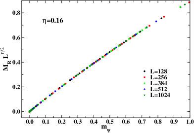
Figure 10: (Color online) Correlation between $M_{R}L^{\eta/2}$ and $m_{\psi}$ for $\eta=0.16$ on lattices with $L$ ranging from 128 to 1024.

5 Discussion and conclusions

In this paper we have presented a wealth of numerical data aimed at shedding light on the phase structure of the $2D$ $Z(5)$ vector model. By means of a Monte Carlo cluster updating algorithm, designed to work for $Z(N)$ models with odd $N$, we have outlined a scenario compatible with the existence of three phases: disorder (small $\beta$), massless or BKT (intermediate $\beta$), order (large $\beta$). We have determined

• the critical points $\beta^{(1)}_{\rm c}$ and $\beta^{(2)}_{\rm c}$ in the infinite volume limit, by means of the FSS of suitable Binder cumulants;

• the critical indices $\beta/\nu$ and $\gamma/\nu$ at the two critical points, by means of the FSS of suitable definitions of the magnetization and of its susceptibility.

The determination of $\beta^{(2)}_{\rm c}$ has been cross-checked with the infinite volume extrapolation of the (volume dependent) pseudocritical couplings of the second transition, assuming essential scaling. We have found the following values of the critical couplings: $\beta^{(1)}_{\rm c}=1.0510(10)$ and $\beta^{(2)}_{\rm c}=1.1048(10)$. As mentioned in the Introduction, values of the critical points are related by the duality transformations. In the Appendix we check, via the duality, the accuracy of our predictions and show that our determination of the critical couplings is in rather good agreement with it.

The determination of the index $\eta^{(1)}=2-\gamma/\nu$ at the first transition has been cross-checked with the effective $\eta$ index method. The values of the index $\gamma/\nu$ at both critical points agree well with theoretical predictions obtained for the Villain formulation [5] thus supporting the conjecture that both standard and Villain formulations are in the same universality class. The behavior of the complex magnetization as well as the two-point correlation function strongly indicate that the intermediate phase is a massless phase whose symmetry is $U(1)$. Moreover, using spin-wave–vortex approximation and conventional perturbation theory one can calculate the two-point correlation function analytically and extract the perturbative beta-function in the intermediate phase. It turns out that the beta-function vanishes in this phase - a property which further supports the presence of the BKT transition and massless phase.

For completeness, we have tested a scenario in which both transitions are second order. In this case, the infinite volume extrapolation of the pseudocritical couplings should obey

$$\beta^{(1,2)}_{\rm pc}=\beta^{(1,2)}_{\rm c}+\frac{A}{L^{\frac{1}{\nu}}}\quad,$$

whereas the overlap method of the Binder cumulants should work when data are plotted against $(\beta-\beta_{c})L^{\frac{1}{\nu}}$. Under these conditions, we found

$$\beta^{(1)}_{\rm c}=1.0425(25)\;, \;\;\;1/\nu^{(1)}=0.50(5)\;,$$

$$\beta^{(2)}_{\rm c}=1.1075(25)\;, \;\;\;1/\nu^{(2)}=0.45(5)\;.$$

In Fig. 11 we show the overlap of the curves for the Binder cumulant $U_{L}^{(M)}$ obtained on various lattices when plotted versus $(\beta-\beta_{\rm c})L^{1/\nu}$, with $1/\nu$ fixed at 0.5 and $\beta_{\rm c}=1.0425$. The quality of the overlap seems to be overall better than in the BKT scenario of Fig. 6, but a closer inspection shows that it is worse in the region near the critical point.

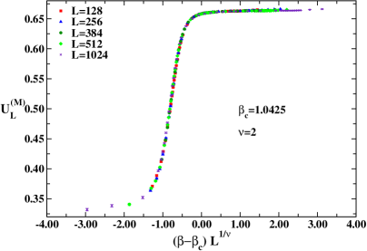
Figure 11: (Color online) Reduced 4-th order Binder cumulant $U^{(M)}_{L}$ versus $(\beta-\beta_{\rm c})L^{1/\nu}$, for $\beta_{\rm c}=1.0425$ and $\nu=2$ on lattices with $L$ ranging from 128 to 1024.

Second order transition at $\beta^{(1)}_{\rm c}$, however, should be excluded by the numerical evidence that the intermediate phase is massless. In particular, two-point correlators tend to vanish at large distances for large volumes, whereas one should expect spontaneous symmetry breaking and non-vanishing values of long distance correlations in the case of second order phase transition. The exclusion of the second order transition at $\beta^{(2)}_{\rm c}$ seems to be a more subtle problem, at least on the numerical side. One should probably simulate the system on larger lattices to reliably distinguish the BKT scenario from the second order one, if we deal with the quantities studied so far. However, one could consider more traditional observables to determine the order of the phase transition. The BKT phase transition is of infinite order. In particular, it is expected that the singular part of the free energy of the $XY$ model behaves like $F_{s}\sim\xi^{-2}$. Hence, all derivatives of the free energy are analytic functions of the temperature. In turn, the second derivative of the free energy shows a finite jump if the system undergoes a second order phase transition. We have decided, therefore, to compute the specific heat $C_{V}$ of the $Z(5)$ model. Figure 12 shows the result of simulations for various lattice sizes. As suggested by this plot, the specific heat shows neither a divergence nor a finite jump. We interpret this behavior as further evidence in favor of the infinite order phase transition. On the theoretical side, the second order transition seems incompatible with the analysis of the dual transformations [15, 16].

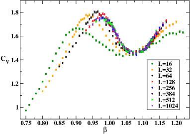
Figure 12: (Color online) Specific heat $C_{V}$ measured on lattices with $L$ ranging from 16 to 1024.

As discussed in the Introduction, in a recent work [19] it has been claimed that the phase transition at $\beta^{(1)}_{\rm c}$ is not a standard BKT phase transition. The main tool in the analysis of Ref. [19] was the helicity modulus $\Upsilon$, which was not considered in this work. The key observation in Ref. [19] was that the helicity modulus does not jump to zero across the phase transition. This property prompted the authors of Ref. [19] to conclude that the phase transition at $\beta^{(1)}_{\rm c}$ is a weaker cousin of the standard BKT transition. Our data indicate that there seem to be no influence of such behavior of the helicity modulus on other characteristic features of the phase transition. Most important on our opinion is the fact that both standard and Villain formulation are still in the same universality class since they show equal critical indices. Moreover, one could consider the critical index which governs the behavior of the helicity modulus [29]

$$\Upsilon\ \sim\ \left(\frac{T-T_{c}}{T_{c}}\right)^{\upsilon}\ ,\;\;\;\;\;\upsilon=2\beta-\eta\nu\ .$$

Our data for the indices $\beta$ and $\eta^{(1)}$ are compatible with a vanishing value of $\upsilon$. Thus, $\Upsilon=const$ right at the critical point. Obviously, $\upsilon=0$ also for the Villain model. The non-vanishing value of $\Upsilon$ at $\beta<\beta^{(1)}_{\rm c}$ seems to characterize rather the high-temperature phase than the massless BKT phase. Indeed, a physical interpretation given in Ref. [19] refers to lack of free vortices in the high-temperature phase of the $Z(5)$ models. It would then be interesting and important to study the dynamics of the vortex–anti-vortex pairs in both formulations. This dynamics can indeed be different. This task, however is beyond the scope of the present paper.

Appendix

Consider general $Z(5)$ vector Potts model with Boltzmann weight given by

$$Q(s)\ =\ 1+2x(\beta)\ \cos\frac{2\pi}{5}s+2y(\beta)\ \cos\frac{4\pi}{5}s\ .$$

Duality transformations read [14]

$$x_{d}(\beta) = (1+2x(\beta)\cos(2\pi/5)+2y(\beta)\cos(4\pi/5))/(1+2x(\beta)+2y(\beta))\ ,$$

$$y_{d}(\beta) = (1+2x(\beta)\cos(4\pi/5)+2y(\beta)\cos(2\pi/5))/(1+2x(\beta)+2y(\beta))\ .$$

The initial couplings $x(\beta)$ and $y(\beta)$ can be calculated from the Fourier transform of the original Boltzmann weight and in our case they are given by

$$x(\beta)\ = \ (-1-\sqrt{5}+(-1+\sqrt{5})e^{\frac{\sqrt{5}\beta}{2}}+2e^{\frac{1}{4}(5+\sqrt{5})\beta})/(4+4e^{\frac{\sqrt{5}\beta}{2}}+2e^{\frac{1}{4}(5+\sqrt{5})\beta})\ ,$$ (17)

$$y(\beta)\ = \ (-1+\sqrt{5}-(1+\sqrt{5})e^{\frac{\sqrt{5}\beta}{2}}+2e^{\frac{1}{4}(5+\sqrt{5})\beta})/(4+4e^{\frac{\sqrt{5}\beta}{2}}+2e^{\frac{1}{4}(5+\sqrt{5})\beta})\ .$$ (18)

It follows that

$$x_{d}(\beta)\ = \ e^{\frac{1}{4}(-5+\sqrt{5})\beta}\ ,$$ (19)

$$y_{d}(\beta)\ = \ e^{-\frac{1}{4}(5+\sqrt{5})\beta}\ .$$ (20)

Now, consider original and dual partition functions,

$$Z(x(\beta),y(\beta))\ =\ C(\beta)\ Z(x_{d}(\beta),y_{d}(\beta))\ .$$

They have the same form and differ only by a smooth function $C(\beta)$. Suppose the original partition function is critical at $\beta_{c}^{(1)}$ and $\beta_{c}^{(2)}$. These values correspond to $(x^{(1)},y^{(1)})$ and $(x^{(2)},y^{(2)})$. Let $(x_{d}^{(1)},y_{d}^{(1)})$ and $(x_{d}^{(2)},y_{d}^{(2)})$ be the values of dual couplings at critical points. The interaction in original and dual partition functions is the same. Therefore, numerical values of the critical points in terms of $(x,y)$ and $(x_{d},y_{d})$ should be the same. However, we know from the solution of the self-dual equation (see [14]) that the self-dual point is not a critical point for the vector Potts model. This leaves the only one possibility, that at the critical points one must have

$$x^{(1)}=x_{d}^{(2)}\;,\;\;\;\;\;y^{(1)}=y_{d}^{(2)}$$

and

$$x^{(2)}=x_{d}^{(1)}\;,\;\;\;\;\>y^{(2)}=y_{d}^{(1)}\;.$$

Results for critical points reported in the text are $\beta_{c}^{(1)}=1.051$ and $\beta_{c}^{(2)}=1.1048$. So, we easily find from (17)-(20)

$$x(1.051)=0.466532\;, x_{d}(1.1048)=0.46608$$

$$y(1.051)=0.136626\;, y_{d}(1.1048)=0.135523$$

and

$$x(1.1048)=0.485097\;, x_{d}(1.051)=0.483733$$

$$y(1.1048)=0.149612\;, y_{d}(1.051)=0.149378\;.$$

References

- [1] V. L. Berezinsky, Sov. Phys. JETP 32 (1971) 493.
- [2] J. Kosterlitz, D. Thouless, J. Phys. C 6 (1973) 1181.
- [3] J. Kosterlitz, J. Phys. C 7 (1974) 1046.
- [4] F. Y. Wu, Rev. Mod. Phys. 54 (1982) 235.
- [5] S. Elitzur, R. B. Pearson, J. Shigemitsu, Phys. Rev. D 19 (1979) 3698.
- [6] M. B. Einhorn, R. Savit, E. Rabinovici, Nucl. Phys. B 170, 16 (1980).
- [7] C. J. Hamer, J. B. Kogut, Phys. Rev. B 22 (1980) 3378.
- [8] B. Nienhuis, J. Statist. Phys. 34 (1984) 731.
- [9] L. P. Kadanoff, J. Phys. A 11 (1978) 1399.
- [10] J. Fröhlich, T. Spencer, Commun. Math. Phys. 81 (1981) 527.
- [11] Y. Tomita, Y. Okabe, Phys. Rev. B 65 (2002) 184405 [arXiv:cond-mat/0202161].
- [12] B. Svetitsky, L. Yaffe, Nucl. Phys B 210 (1982) 423.
- [13] A. Ukawa, P. Windey, A. Guth, Phys. Rev. D 21 (1980) 1013.
- [14] F. Y. Wu, J. Phys. C 12 (1979) L317.
- [15] J. l. Cardy, J. Phys. A 13 (1980) 1507.
- [16] E. Domany, D. Mukamel, A. Schwimmer, J. Phys. A 13 (1980) L311.
- [17] P. Ruján, G. O. Williams, H. L. Frisch, G. Forgács, Phys. Rev. B 23 (1981) 1362; H. H. Roomany, H. W. Wyld, Phys. Rev. B 23 (1981) 1357.
- [18] C. M. Lapilli, P. Pfeifer, C. Wexler, Phys. Rev. Lett. 96 (2006) 140603 [arXiv:cond-mat/0511559]
- [19] S.K. Baek and P. Minnhagen, Phys. Rev. E 82 (2010) 031102 [arXiv:1009.0356 [cond-mat.stat-mech]].
- [20] S.K. Baek, P. Minnhagen and B.J. Kim, Phys. Rev. E 80 (2009) 060101(R) (2009) [arXiv:0912.2830 [cond-mat.stat-mech]].
- [21] M. Hasenbusch, J. Stat. Mech. 2008 P08003.
- [22] O. Borisenko, G. Cortese, R. Fiore, M. Gravina, A. Papa, Critical properties of the two-dimensional Z(5) vector model, PoS LATTICE2010 (2010) 274.
- [23] O. Borisenko, M. Gravina, A. Papa, J. Stat. Mech. 2008 (2008) P08009 [arXiv:0806.2081 [hep-lat]].
- [24] O. Borisenko, R. Fiore, M. Gravina, A. Papa, J. Stat. Mech. 2010 (2010) P04015 [arXiv:1001.4979 [hep-lat]].
- [25] R. Kenna and A. C. Irving, Nucl. Phys. B 485 (1997) 583 [arXiv:hep-lat/9601029].
- [26] M. Hasenbusch, J. Phys. A 38 (2005) 5869 [arXiv:cond-mat/0502556v2 [cond-mat.stat-mech]].
- [27] M. S. S. Challa, D. P. Landau and K. Binder, Phys. Rev. B 34 (1986) 1841.
- [28] D. Loison, J. Phys.: Condens. Matter 11 (1999) L401.
- [29] M. E. Fisher, M. N. Barber, D. Jasnow, Phys. Rev. A 8 (1973) 1111.