KEK Preprint 2010-41

FTUV-10-1129

Measuring Anomalous Couplings in $H\to WW^{\ast}$ Decays at the International Linear Collider

Yosuke Takubo^(a), Robert N. Hodgkinson^(b), Katsumasa Ikematsu^(a),

Keisuke Fujii^(a), Nobuchika Okada^(c), and Hitoshi Yamamoto^(d)

^(a)High Energy Accelerator Research Organization (KEK), Tsukuba, Japan
^(b)Departamento de Fìsica Teòrica and IFIC, Universitat de València–CSIC, València, Spain
^(c)Department of Physics and Astronomy, University of Alabama, Tuscaloosa, AL 35487, USA
^(d)Department of Physics, Tohoku University, Sendai, Japan

1 Introduction

The announcement of the discovery of the Higgs boson candidate at the Large Hadron Collider (LHC), has elevated the question of its properties to the top of the list of questions in high energy physics [1, 2]. The Higgs field is crucial to the Standard Model (SM), as it provides the mechanism for electroweak (EW) symmetry breaking and gives rise to the masses of both the $W^{\pm}$ and $Z$ gauge bosons and all charged fermions when it develops a vacuum expectation value (VEV).

In practice, the discovery of a SM-like Higgs boson is only the beginning of the story. Over the last thirty years, a number of alternative models have been proposed, notably low-energy supersymmetry and models with extra dimensions, which attempt to resolve the so-called hierarchy problem of the SM. It is crucial to measure the properties of the Higgs particle in order to ascertain to which, if any, of the proposed models it belongs. Of particular importance will be the task of verifying that the discovered Higgs boson candidate really is the particle responsible for EW symmetry breaking and the generation of fermion masses.

Indeed, it is notable that one of the “gold plated” Higgs boson discovery channels at the LHC involves production of the Higgs particle through gluon fusion, followed by its decay into photon pairs, i.e. $gg\to H\to\gamma\gamma$. This channel involves loop-induced couplings in both production and decay and the discovery of such a resonance tells us very little about EW symmetry breaking! For this, accurate measurements of the Higgs boson couplings to the EW gauge bosons must be made. The LHC can be used to extract some information on the Higgs boson coupling to $Z$ bosons using the decay $H\to ZZ\to(l^{+}l^{-})(l^{\prime+}l^{\prime-})$ [5], since this final state can be efficiently triggered; effects of anomalous $HW^{+}W^{-}$ couplings can also be probed through their contribution to $WW$ scattering [6] and the gauge-boson fusion Higgs production mechanism [7]. For a direct measurement of the $HW^{+}W^{-}$ coupling, however, the best environment is a lepton collider, such as the International Linear Collider (ILC).

In an electron-positron collider such as the ILC, Higgs bosons are predominantly produced through EW interactions, either through Higgs-strahlung from virtual $Z$-bosons or through gauge boson fusion; such reactions can therefore be used to probe anomalous Higgs-gauge-gauge couplings [8]. Furthermore, the clean environment of a lepton collider also allows for studies based on the asymmetries in the decays of the Higgs boson [9]. For an additional heavy Higgs boson (with mass $\>\raisebox{-2.15277pt}{$\stackrel{{\scriptstyle\textstyle>}}{{\sim}}$}\>200$ GeV), if any, the authors of [10] have proposed to accurately measure the couplings instead at a future photon collider.

If, as we expect, the underlying theory is gauge invariant, then anomalous $HWW$ couplings necessarily imply anomalous contributions to the $HZZ,\ H\gamma\gamma$, and mixed $HZ\gamma$ vertices. Whilst measurements of anomalous Higgs boson couplings to the neutral vector bosons may make use of the very high rates of the Higgs-strahlung process, determining the structure of the $HW^{+}W^{-}$ vertex relies on either the gauge-boson fusion production process or on the decay $H\to WW^{\ast}$. Furthermore, these measurements should be performed independently of one another, as a test of the underlying gauge invariance. In this paper we concentrate on the decay process for two reasons; firstly, the differential cross sections considered do not depend on the additional $HNN,\ N=Z,\gamma$ anomalous couplings at leading order and secondly, this process allows us to study the effects of CP-violating parameters. In contrast, since the final state forward neutrinos are not measured in the gauge-boson fusion process $e^{+}e^{-}\to H\nu\bar{\nu}$, this process has no sensitivity to CP-violating parameters; furthermore, there are large backgrounds from the related process $e^{+}e^{-}\to He^{+}e^{-}$, where the final state electrons also escape detection, which introduces a significant dependence on the $HNN$ anomalous couplings.

In particular, we study the feasibility of measurements for anomalous Higgs boson couplings to $W^{+}W^{-}$ pairs using $ZH$ production followed by $H\to WW^{\ast}$ and $Z\to\nu\nu$ at the ILC, based on realistic Monte Carlo simulations. We stress that this is the first full simulation study of its kind using a full detector simulator based on geant4 and a real event reconstruction chain. The Higgs production mechanism clearly depends on the presence of anomalous $HZZ$ and $HZ\gamma$ couplings, however the distributions of the Higgs boson decay products which constitute our signal do not. The only possible effect of anomalous $HNN$ couplings in the production mechanism is a change in the overall rate $e^{+}e^{-}\to ZH\to ZWW^{\ast}$ and can easily be measured at relatively low integrated luminosities [8]. Hence, we feel justified in neglecting the effect of these couplings in our analysis focusing on the Higgs decay $H\to WW^{\ast}$.

The structure of our paper is as follows. In the next section we outline the effective interaction Lagrangian under discussion and present analytic formulas for the relevant differential decay rates. In Section 3, we present details of the Monte Carlo simulation and results of the analysis. We discuss these results and a simple example of new physics model which give rise to the effective interaction Lagrangian in Section 4. The final section is reserved for summary and conclusions.

2 Physics Model

We may parametrise the relevant terms of the general interaction Lagrangian, which couples the Higgs boson to EW vector bosons in a Lorentz-symmetric fashion, as

$$\mathcal{L}_{\rm HWW}=2M_{W}^{2}\left(\frac{1}{v}+\frac{a}{\Lambda}\right)H\ W_{\mu}^{+}W^{-\mu}+\frac{b}{\Lambda}H\ W^{+}_{\mu\nu}W^{-\mu\nu}+\frac{\tilde{b}}{\Lambda}H\ \epsilon^{\mu\nu\sigma\tau}W^{+}_{\mu\nu}W^{-}_{\sigma\tau}\ ,$$ (2.1)

where $M_{W}$ is the mass of the $W$-boson, $W_{\mu\nu}^{\pm}$ is the usual gauge field strength tensor, $\epsilon^{\mu\nu\sigma\tau}$ is the Levi-Civita tensor, $v$ is the VEV of the Higgs field, $a,b,\tilde{b}$ are real dimensionless coefficients and $\Lambda$ is a cutoff scale. The SM interaction is recovered in the limit $a,b,\tilde{b}\to 0$. The dimensionless couplings $b,\tilde{b}$ parametrise the leading dimension-five non-renormalisable interactions, which we assume are due to contributions arising from some new physics at the scale $\Lambda$. The dimensionless coupling $a$ represents corrections to the SM term, assumed to originate at the same scale $\Lambda$. The Lagrangian (2.1) is not by itself gauge invarient; to restore explicit gauge invarience we must also include the corresponding anomalous couplings of the Higgs boson to $Z$ bosons and photons.

We will assume the Higgs boson mass to be $M_{H}<2M_{W}$, being consistent with the recent discovery of the Higgs boson candidate at the LHC [1, 2], so that the decay to real $W^{+}W^{-}$ pairs is kinematically forbidden; the anomalous couplings may however contribute to the decay $H\to WW^{\ast}$ with distinct signatures. The $a$ parameter is simply a rescaling of the SM coupling and therefore manifests itself as a shift in the overall partial width for this channel. By comparison, the non-renormalisable coupling $b$ has a different Lorentz structure to the SM term and leads to a change in the ratio of couplings to the transverse or longitudinal components of the gauge bosons. Finally, the coupling $\tilde{b}$ introduces a CP-violating operator which can affect angular correlations, as discussed below.

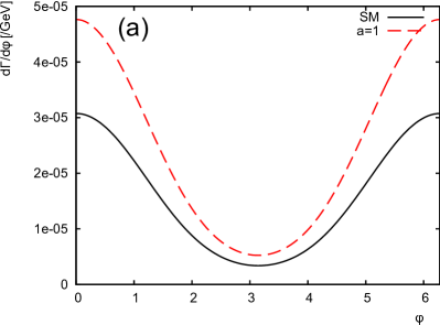
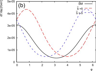
Figure 1: The $\phi$-distribution of the decay $H\to WW^{\ast}\to 4j$ with the inclusion of anomalous couplings. (a) The SM curve along with that for $a=1$, $b=\tilde{b}=0$, same for both distributions. (b) The SM result with the cases $\tilde{b}=\pm 5$, $a=\tilde{b}=0$, $\Lambda=1$ TeV; the position of the minimum is now shifted as discussed in the text.

Assuming all final state fermions to be massless, the differential partial width for the decay chain $H\to WW^{\ast}\to 4j$ as a function of the on-shell $W$-boson momentum $p_{W}$ and the azimuthal angle between the up-type quark and anti-quark $\phi$ (with axis of rotation in the direction of the $W^{+}$ momentum) is given by

$$\frac{d^{2}\Gamma}{dp_{W}d\phi} = \left(N_{c}\sum_{\stackrel{{\scriptstyle i=u,c}}{{j=d,s,b}}}|V_{ij}|^{2}\right)^{2}\frac{1}{2M_{H}\ 2M_{W}\Gamma_{W}}\frac{M_{W}^{10}k^{2}p_{W}^{2}}{(k^{2}-M_{W}^{2})^{2}\pi^{5}E_{W}v^{6}}$$ (2.2)

$$\hskip 28.45274pt\times\left[\frac{c_{0}}{36}+\left(\frac{c_{\phi}e^{i\phi}+c_{\phi}^{\ast}e^{-i\phi}}{512}\right)+\left(\frac{c_{2\phi}e^{i2\phi}+c_{2\phi}^{\ast}e^{-i2\phi}}{288}\right)\right]\ ,$$

where $N_{c}=3$ is the number of colors, $V_{ij}$ is the Cabibbo-Kobayashi-Maskawa quark mixing matrix, $\Gamma_{W}$ is the $W$-boson width, $E_{W}=\sqrt{M_{W}^{2}+p_{W}^{2}}$ is the energy of the on-shell $W$-boson and $k^{2}=(M_{H}-E_{W})^{2}-p_{W}^{2}$ is the invariant squared mass of the off-shell $W$-boson. The coefficient functions $c_{0},\ c_{\phi},\ c_{2\phi}$ can be written in terms of two dimensionless combinations of parameters,

$$c_{0} = |T|^{2}+\frac{1}{2}L^{2}\ ,$$

$$c_{\phi} = \pi^{2}TL\ ,$$

$$c_{2\phi} = T^{2}\ ,$$ (2.3)

where the real function $L$ is due to contribution from longitudinally polarized on-shell $W$-bosons and the complex function $T$ from transversely polarized bosons. Explicitly, they are given by

$$T = \left(1+\frac{av}{\Lambda}\right)-\frac{bv}{\Lambda}\frac{\left(p^{\mu}_{W}k_{\mu}\right)}{M_{W}^{2}}-i\frac{2M_{H}p_{W}}{M_{W}^{2}}\frac{v\;\tilde{b}}{\Lambda}\ ,$$

$$L = \left(1+\frac{av}{\Lambda}\right)\frac{\left(p^{\mu}_{W}k_{\mu}\right)}{M_{W}k}-\frac{bv}{\Lambda}\frac{\left(\left(p^{\mu}_{W}k_{\mu}\right)^{2}-M_{H}^{2}p_{W}^{2}\right)}{M_{W}^{3}k}\ ,$$ (2.4)

where $k_{\mu}$ is the $4$-momentum of the off-shell $W$-boson and $k=\sqrt{k_{\mu}k^{\mu}}$. The 4-vector product $p^{\mu}_{W}k_{\mu}$ can be expanded as $p^{\mu}_{W}k_{\mu}=M_{H}E_{W}-M_{W}^{2}$.

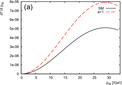
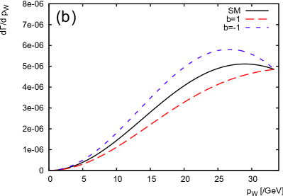
Figure 2: The $p_{W}$ distribution of the decay $H\to WW^{\ast}\to 4j$ with the inclusion of anomalous couplings. (a) The SM curve along with that for $a=1$, $b=\tilde{b}=0$, $\Lambda=1$ TeV. (b) The SM result with the cases $b=\pm 1$, $a=\tilde{b}=0$, $\Lambda=1$ TeV.

We see that for $\tilde{b}=0$, all coefficients $c_{0},\ c_{\phi},\ c_{2\phi}$ are real and the partial decay width is a function of cosines only. In the SM limit, the magnitudes of the transverse function $T$ and the longitudinal function $L$ are approximately equal, assuming a $W$-boson energy of the order of the $W$ mass, $E_{W}\sim M_{W}$. From (2), in this limit we have the ratio of coefficients $c_{\phi}/c_{2\phi}\sim\pi^{2}$ so that the $\cos\phi$ term dominates, the minimum of the distribution is seen to be at $\phi_{\rm min}=\pi$. Non-zero values of $\tilde{b}$ shift the minimum of the $\phi$ distribution to $\phi_{\rm min}=\pi+\delta$ with $\delta={\rm arg}(T)$. This effect is illustrated in Fig. 1, where we plot the $\phi$-dependence of the partial width in both the SM and taking $a=1,b=\tilde{b}=0$ (Fig. 1 (a)) and $a=0,\tilde{b}=\pm 5$ (Fig. 1 (b)), with $\Lambda=1$ TeV.

The energy of the on-shell $W$ boson in the decay $H\to WW^{\ast}$ is not fixed by kinematic constraints. After integrating (2.2) over $\phi$ we see that only the $c_{0}$ term contributes to the differential decay rate $d\Gamma/dp_{W}$. The presence of the anomalous couplings $b,\tilde{b}$ modifies the energy-dependence of this expression through the $L$ and $T$ functions, as shown in Fig. 2, which compares the effect of non-zero $a$ and $b$ terms. In particular, the contribution of $b$ is seen to vanish at the kinematic limit of the distribution.

3 Monte Carlo Simulation

3.1 Simulation Conditions and Tools

For the simulation of the measurement of the anomalous $HWW$ couplings, we take the Higgs mass to be $120\,$GeV along with a center of mass energy of $250\,$GeV and an integrated luminosity of $250\,$fb^-1 as assumed in the Letters of Intent (LoI) for the ILC detectors [12, 13, 14]. Notice that for a Higgs mass of $120\,$GeV the $ZH$ cross-section attains its maximum at around this energy and the branching ratio for $H\to WW^{*}$ decay is 15.0%, which is subdominant. The angular analyses and $W$ momentum measurement discussed in the previous section necessitate the identification of the four jets from the $H\to WW^{\ast}$ decay and their correct pairing. Given the branching fraction of this decay mode and the additional combinatorial background in the jet paring which would otherwise hamper the analyses, we require the associated $Z$ to decay into $\nu\bar{\nu}$. Our signal thus consists of four jets plus missing energy. Consequently, four fermion final states such as $\nu\nu qq$, $qq\ell\nu$, $\ell\ell\ell\ell$, $qq\ell\ell$, and $qqqq$, primarily coming from $WW$ and $ZZ$ production, comprise the SM background. In order to suppress these backgrounds, which would otherwise dominate in this study, we use 80% right-handed polarization for the electron beam and 30% left-handed polarization for the positron beam in the following analysis.

The signal events $ZH\to\nu\nu WW^{\ast}$ were generated using Physsim [15], with the cutoff scale $\Lambda$ taken to be 1 TeV when the anomalous couplings were switched on. $ZH\to\nu\nu H$ events for decay modes other than $H\to WW^{\ast}$ were generated by WHIZARD, together with all the other SM backgrounds. In both generators, initial-state radiation and beamstrahlung have been included in the event generation. The beam energy spread was set to 0.28% for the electron beam and 0.18% for the positron beam. We have ignored the finite crossing angle between the electron and positron beams. In the event generation, helicity amplitudes were calculated using the HELAS library [16], which allows us to deal with the effect of gauge boson polarizations properly. The event generator Pythia6.409 [17] was used for parton-showering and hadronization. The generator data for the SM background had been prepared as a common data sample for the LoI studies and stored in the StdHep format [18] at SLAC. The SM background sample consists of all the SM processes with up to 4 fermions in the final state, which is about 10 million events in total. Since the cross-section of 6 fermion events is small compared to that of the signal at $\sqrt{s}=250$ GeV and can be rejected easily, we ignored these events.

The 4-momenta of the (quasi-)stable particles after parton-showering and hadronization were fed into a geant4-based full detector simulator called Mokka [19], in which ILD_00 is implemented as the detector model [12]. The ILD_00 detector model consists, from inside to outside, of a very thin 6-layer vertex detector with a point resolution of about $3\,\mu$m, silicon internal and forward trackers, a time projection chamber (TPC) having about 200 sample points with a point resolution of $100\,\mu$m or better, silicon external and endcap trackers, ultra high granularity electro-magnetic and hadron calorimeters, a superconducting solenoid of $3.5\,$T, and return yokes interleaved with muon detectors. With this detector model, we expect the transverse momentum resolution ($\Delta(1/p_{\mathrm{T}})=\Delta p_{\mathrm{T}}/p_{\mathrm{T}}^{2}$) to be $2.0\times 10^{-5}$ GeV^-1 asymptotically, rising to $9.0\times 10^{-5}$ GeV^-1 at 10 GeV, and to $9.0\times 10^{-4}$ GeV^-1 at 1 GeV.

The generated detector hits and signals were processed through a real event reconstruction program called MarlinReco implemented in the Marlin framework [20]. In the event reconstruction, charged particle tracks were reconstructed from tracker hits by a realistic track finder and a Kalman-filter-based track fitter, taking into account signal overlapping as well as energy loss and multiple scattering. Calorimeter hits were then clustered and combined with the tracker information to perform a particle flow analysis (PFA) [21] to achieve the best jet energy resolution. The jet energy resolution for $45\,$GeV jets from $Z\to q\bar{q}$ events is estimated to be 3.7%, which improves to about 3% for $100\,$GeV jets. Jet clustering was done with the Durham algorithm [22], and the resultant jets were flavor-tagged on a jet-by-jet basis with the LCFIVertex package [23] after vertex finding with the ZVTOP algorithm [24].

3.2 Event Selection

The goal of our event selection is to isolate the signal events with four jets plus missing energy originating from $ZH$ production followed by $H\to WW^{\ast}$ and $Z\to\nu\bar{\nu}$ decays. We thus started our event selection by forcing all the events to cluster into four jets by adjusting the $Y_{\rm cut}$ value [22]. The Higgs boson and on-shell $W$ boson masses were then reconstructed by paring these four jets so as to minimize the $\chi^{2}$ function defined by

$$\chi^{2}=\frac{(^{\mathrm{rec}}M_{H}-M_{H})^{2}}{\sigma_{H}^{2}}+\frac{(^{\mathrm{rec}}M_{W}-M_{W})^{2}}{\sigma_{W}^{2}},$$ (3.5)

where ${}^{\mathrm{rec}}M_{H}$ is the reconstructed Higgs mass, $M_{H}$ is the input Higgs mass (120 GeV), ${}^{\mathrm{rec}}M_{W}$ is the reconstructed on-shell $W$ mass, $M_{W}$ is the nominal $W$ mass ($80.4\,$GeV) and $\sigma_{H(W)}$ is the mass resolution for the Higgs @($W$).

After the mass reconstruction, we required the reconstructed Higgs mass (${}^{\mathrm{rec}}M_{H}$) to lie in the range $110\,\mathrm{GeV}<\,^{\mathrm{rec}}M_{H}<130\,\mathrm{GeV}$. Since we assume a $Z$ boson decaying into a neutrino pair in the signal event, resulting in a missing mass peak at the $Z$ mass, we required a missing mass in the range $70\,$GeV $<\,^{\mathrm{miss}}M<140\,$ GeV.

The main backgrounds in this analysis are from $e^{+}e^{-}\to WW$ and $ZZ$. The angular distributions of these processes have peaks in the forward and backward regions. For this reason, we required the angle of the reconstructed Higgs boson with respect to the beam axis ($\cos\theta_{H}$) to be $|\cos\theta_{H}|<0.95$. We then looked at the $Y$-value for the forced 4-jet clustering, which is expected to be small for $\nu\nu qq$ and $\nu\nu\ell\ell$ events having only two “partons” in their final states. We therefore selected events with $Y_{\mathrm{-}}>0.0005$, where $Y_{\mathrm{-}}$ is the threshold $Y$-value at which the number of jets changes four to three. After the selection cuts described so far, the dominant background became $\ell\nu qq$. The lepton in the $\ell\nu qq$ final state comes from the leptonic decay of a $W$ and has a larger energy than leptons from jets. We hence required the maximum track energy ($E_{\mathrm{trk}}$) to be below 30 GeV.

Since we are focusing our attention on the $H\to WW^{\ast}$ decay in this analysis, the $ZH\to\nu\nu bb$ process is a background to be discarded. We thus rejected $ZH\to\nu\nu bb$ events by requiring the number of $b$-tagged jets (${}^{\mathrm{4-jet}}N_{b}$) to be ${}^{\mathrm{4-jet}}N_{b}\leq 1$. Since the $ZH\to\nu\nu bb$ channel has two jets in the final state, candidate events were further jet-clustered into two jets and then required to have no $b$-tagged jets, ${}^{\mathrm{2-jet}}N_{b}=0$.

After all the selection cuts, we performed a likelihood analysis as follows. We used ${}^{\mathrm{miss}}M$, $\cos\theta_{H}$, $Y_{-}$, ${}^{\mathrm{4-jet}}N_{b}$, and the number of charged tracks as the input variables of the likelihood function and tuned the likelihood cut position to maximize signal significance. We obtained a maximum signal significance of $7.6$ at a likelihood cut position $\mathcal{L}_{\mathrm{cut}}=0.79$. Figure 3 shows the reconstructed Higgs mass distribution after all cuts. Fitting the distribution with a double Gaussian plus a second order polynomial, we estimated the expected accuracy of the branching ratio BR($H\to WW^{\ast}$) to be $15.7\%$, assuming that the measurement accuracy of the $ZH$ cross-section is $2.5\%$ [12]. The branching ratio can be determined to an accuracy of $5\%$, however, by using processes with leptonic decays of the $W$ [25]. The number of events before and after the selection cuts are summarized in Table 1.

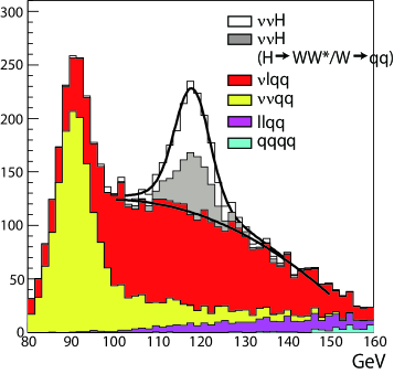
Figure 3: Distribution of the reconstructed Higgs mass after selection cuts.

Process	No cut	After cuts	$\mathcal{L}_{\mathrm{cut}}>0.79$	$N_{c}=2$
$\nu\nu H(H\to\mathrm{all})$	10,634	1,518	756	546
$\nu\nu H(H\to WW^{\ast}\to$ 4-jet)	680	512	348	258
$\ell\ell\ell\ell$	753,964	46	0	0
$qqqq$	378,726	8	3	2
$\ell\ell qq$	335,762	409	94	70
$\nu\ell qq$	299,866	8,571	1,063	692
$\nu\nu\ell\ell$	103,704	3	0	0
$\nu\nu qq$	63,649	1,090	207	110

Table 1: Cut summary.

3.3 Analysis Results

We investigated the distributions of the variables sensitive to the anomalous couplings. The distributions of the $W$ boson momenta in the Higgs rest-frame ($p_{W}$) and the jet angle in the $W$ boson rest-frame were plotted after selection cuts. The jet angle distributions were plotted for the on-shell ($\cos\theta_{j1}$) and off-shell $W$ bosons ($\cos\theta_{j2}$) separately. We also examined the distribution of the angle between the two $W$ boson decay planes ($\phi_{\mathrm{plane}}$) corresponding to that between the two up-type quarks from the decays of the $W$ bosons. We applied double $c$-tagging to select the two up-type quarks ($c$ quark) in $ZH\to\nu\nu WW^{*}\to\nu\nu cscs$, where the selection efficiency was 88% as shown in Table 1. The $\phi_{\mathrm{plane}}$ was histogrammed using the two $c$-tagged jets, without identifying their charges. Distributions for the $ZH$ events were obtained, evaluating the contamination from the SM backgrounds by fitting the Higgs mass distribution for each $\phi_{\mathrm{plane}}$ bin. Since the branching ratio of the Higgs to channels other than $H\to WW^{\ast}$ will be determined with much better accuracies than the statistical errors shown on the distributions [25], we subtracted the background from these decay modes ignoring their systematic errors on the cross-section to obtain the distributions of $p_{W}$, $\cos\theta_{j1}$, $\cos\theta_{j2}$, and $\phi_{\mathrm{plane}}$ for $ZH\to\nu\nu WW^{\ast}$ events.

As mentioned above, if the anomalous couplings exist in $H\to WW^{\ast}$, there should also be similar anomalous couplings of the same origin in $H\to ZZ^{\ast}$ and $Z\gamma$ decays. In order to make sure that the possible anomalies in the $HZZ$ and $HZ\gamma$ couplings would not affect our measurement of the anomalous $HWW$ couplings, we have evaluated the contamination from the $H\to ZZ^{\ast}$ and $Z\gamma$ decays. After all the selection cuts, the contamination of the $H\to WW^{\ast}$ sample from the $H\to ZZ^{\ast}$ and $H\to Z\gamma$ decays was only 23 events in the SM case and within the statistical error.

As long as the anomalous couplings stem from the same origin, it is reasonable to expect that the anomalous $HZZ$ and $HZ\gamma$ couplings, are of the same order to the anomalous $HWW$ couplings. The effect of the anomalous $HZZ$ and $HZ\gamma$ couplings on the contamination from the $H\to ZZ^{\ast}$ and $H\to Z\gamma$ decays (only the 23 events in the SM) in the $H\to WW^{\ast}$ sample can be ignored, since, if the effect on the $H\to ZZ^{\ast}$ and $H\to Z\gamma$ contamination is sizable, the effect on the $H\to WW^{\ast}$ should be much larger for our $H\to WW^{\ast}$ sample as long as the interference term with the SM amplitude dominates the anomalous coupling term squared. We thus conclude that the possible anomalous $HZZ$ and $HZ\gamma$ couplings will not affect the sensitivity of our measurement of the anomalous $HWW$ couplings using the $H\to WW^{\ast}$ decay.

It should also be worth noting that we can separately study the effect including its size of the anomalous $HZZ$ and $HZ\gamma$ couplings, for instance by measuring the production cross section: $e^{+}e^{-}\to ZH$ without looking at the Higgs decay at all, using the recoil mass technique [12].

To estimate the sensitivity to the Higgs anomalous couplings, the distributions of $p_{W}$, $\cos\theta_{j1}$, $\cos\theta_{j2}$, and $\phi_{\mathrm{plane}}$ for events with non-zero anomalous couplings were compared with the SM case. For the comparison we varied two of the parameters $a,\ b$, and $\tilde{b}$, whilst the third was set to zero. We then drew probability contours for $\Delta\chi^{2}=1,\ 2.28$ and $5.99$, corresponding to $39\%,\ 68\%$ and $95\%$ confidence levels (C.L.) respectively, as in Figs. 4 through 6.

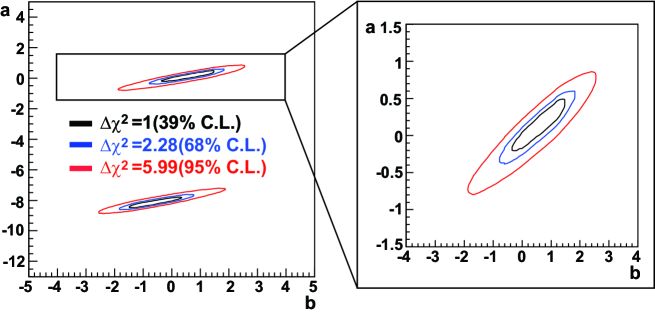
Figure 4: Probability contours for $\Delta\chi^{2}=$ 1, 2.28, and 5.99 in the $a$-$b$ plane, which correspond to 39%, 68%, and 95% C.L., respectively.

The contour plot in the $a$-$b$ plane (Fig. 4) shows a linear correlation between $a$ and $b$ due to changes in absolute value of the $ZH\to\nu\nu WW^{\ast}$ cross section, which increases with $a$ but decreases with increasing $b$. Note that with our conventions $a\simeq-4.1$ cancels the SM coupling of the Higgs to $W^{+}W^{-}$, which means that taking $a\simeq-8.2$ effectively reverses the sign of the SM coupling term. If we reverse the sign of the $b$ term in addition, we hence obtain exactly the same distribution provided that the other parameter, $\tilde{b}$, is kept at zero. For this reason we observe a second allowed region in Fig. 4, connected to the first region (containing the SM point $a=b=0$) by a $180^{\circ}$ rotation about $(a,b)=(-4.1,0)$.

By the same token, we have two allowed regions for the contours in the $a$-$\tilde{b}$ plane as plotted in Fig. 5.

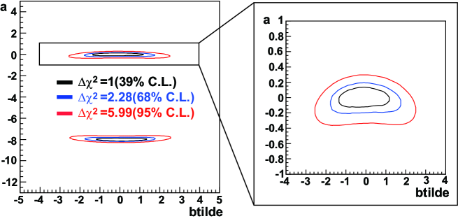
Figure 5: Contours similar to Fig. 4 plotted in the $a$-$\tilde{b}$ plane.

The additional mirror symmetry of the contours about $\tilde{b}=0$ is present because we did not identify the charge of the charm jets for the $\phi_{\mathrm{plane}}$ measurement. The prospects for resolving this additional degeneracy by measuring the jet charge are discussed in Section 4.1.

Finally, Fig. 6 shows the contours in the $b$-$\tilde{b}$ plane for $a=0$. We observe that these contours are also symmetric under the replacement $\tilde{b}\to-\tilde{b}$, again due to the non-identification of the jet charge.

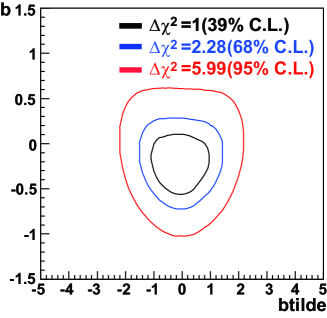
Figure 6: Contours similar to Fig. 5 plotted in the $b$-$\tilde{b}$ plane.

4 Discussions

4.1 Charge identification of $c$-jets

If the charge of $c$-jets can be identified, the shape of the $\phi_{\mathrm{plane}}$ distribution will change depending on the sign of $\tilde{b}$. For this reason, it might be possible to identify the sign of $\tilde{b}$ by using the charge identification of $c$-jets. Since the charge identification of $b$- and $c$-jets is considered possible at the ILC by measuring the number of positive and negative charged tracks in the jet clusters, we investigated the sensitivity to the anomalous coupling including identification of the jet charge.

The efficiency of the charge identification for $c$-jets was assumed to be $14.6\%$ [23] and the same efficiency was used for the backgrounds. We ignored the probability to mis-identify the jet charge as the opposite sign. If we require that the charge of at least one $c$-jet candidate is identified, $27\%$ of $ZH\to\nu\nu WW^{\ast}\to\nu\nu cscs$ events can be selected. By using these events, the $\phi_{\mathrm{plane}}$ distribution was produced considering the relative direction of the positive and negative charge ($\phi_{\mathrm{plane}}^{+-}$). When the charges of both $c$-jet candidates were not identified, $\phi_{\mathrm{plane}}$ was calculated just as the angle between two $c$-jet candidates ($\phi_{\mathrm{plane}}^{00}$). Then, the sensitivity to the anomalous coupling was evaluated by using $p_{W}$, $\cos\theta_{j1}$, $\cos\theta_{j2}$, $\phi_{\mathrm{plane}}^{+-}$, and $\phi_{\mathrm{plane}}^{00}$.

Figure 7 shows the probability contours for $\Delta\chi^{2}=1,\ 2.28,$ and $5.99$ in the $a$-$\tilde{b}$ plane. Here, the integrated luminosity is taken to be 1,000 fb^-1, since the statistics of $ZH\to\nu\nu WW^{*}\to\nu\nu cscs$ are not sufficient to evaluate the background contamination in the $\phi_{\mathrm{plane}}$ distribution after the charge identification with 250 fb^-1. In Fig. 7, we can see the weak linear correlation between $a$ and $\tilde{b}$. The mirror symmetry corresponding to $\tilde{b}\to-\tilde{b}$ is thus broken, although we still have the rotational symmetry corresponding to the combined transformation $(a,\tilde{b})\to(-8.2-a,-\tilde{b})$.

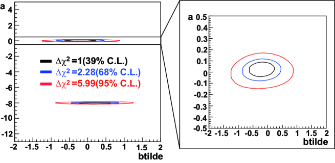
Figure 7: Contours similar to Fig. 5 plotted in the $a$-$\tilde{b}$ plane. Here, the integrated luminosity is assumed as 1,000 fb^-1.

4.2 Theoretical consideration

Here we discuss theoretical possibilities to induce the non-renormalizable interactions in Eq. (2.1) as low energy effective theory. A simple setup is the Randall-Sundrum model [26], in which the gauge hierarchy problem can be solved by virtue of the warped metric. In the effective four dimensional theory of this model, the effective cutoff at the TeV scale emerges as $\Lambda=M_{P}\omega$ with the reduced Planck scale $M_{P}=2.4\times 10^{18}$ GeV and the so-called warp factor $\omega\sim 10^{-15}$ associated with the warped metric. In this model, we can introduce effective higher-dimensional interactions [4]

$${\cal L}_{\rm int}=\sum_{A=1,2}\;c_{A}\;\frac{\phi^{\dagger}\phi}{\Lambda^{2}}\;{\rm tr}\left[{\cal F}_{A}^{\mu\nu}{\cal F}_{A\mu\nu}\right],$$ (4.6)

where $\phi$ is the SM Higgs doublet field, the constants $c_{A}$ are dimensionless parameters, and ${\cal F}_{A}$ are the field strengths of the corresponding SM gauge groups, U(1)_Y and SU(2)_L. After EW symmetry breaking, Eq. (4.6) is rewritten as interactions of the Higgs boson with photons, $Z$- and $W$-bosons,

$${\cal L}_{\rm int} = \frac{c_{WW}}{\Lambda}\left(\frac{v}{\Lambda}\right)HW^{+}_{\mu\nu}W^{-\mu\nu}+\frac{c_{ZZ}}{2\Lambda}HZ^{\mu\nu}Z_{\mu\nu}$$ (4.7)

$$+ \frac{c_{\gamma\gamma}}{\Lambda}\left(\frac{v}{\Lambda}\right)F^{\mu\nu}F_{\mu\nu}+\frac{c_{Z\gamma}}{2\Lambda}\left(\frac{v}{\Lambda}\right)Z^{\mu\nu}F_{\mu\nu},$$

where $W^{+}_{\mu\nu}$, $Z^{\mu\nu}$ and $F^{\mu\nu}$ are the field strengths of the $W$-boson, $Z$-boson and photon respectively. The couplings $c_{WW}$ etc. can be described in terms of the original two couplings $c_{1},\ c_{2}$ and the weak mixing angle $\theta_{w}$ as follows:

$$c_{WW} = c_{2},$$

$$c_{ZZ} = c_{1}\sin^{2}\theta_{w}+c_{2}\cos^{2}\theta_{w},$$

$$c_{\gamma\gamma} = c_{1}\cos^{2}\theta_{w}+c_{2}\sin^{2}\theta_{w},$$

$$c_{Z\gamma} = (-c_{1}+c_{2})\sin\theta_{w}\cos\theta_{w}.$$ (4.8)

We can identify $b=c_{WW}v/\Lambda$. In the same way, we can obtain $\tilde{b}$ in Eq. (2.1) by effective interactions

$${\cal L}_{\rm int}=\sum_{A}\;\tilde{c}_{A}\;\frac{\phi^{\dagger}\phi}{\Lambda^{2}}\;\epsilon^{\mu\nu\rho\sigma}{\rm tr}\left[{\cal F}_{A\mu\nu}{\cal F}_{A\rho\sigma}\right].$$ (4.9)

We can also introduce

$${\cal L}_{\rm int}=c_{0}\;\frac{\phi^{\dagger}\phi}{\Lambda^{2}}\;\left(D^{\mu}\phi\right)^{\dagger}\left(D_{\mu}\phi\right),$$ (4.10)

which gives rise to $a=c_{0}v/\Lambda$ in Eq. (2.1). If we allow $c_{A},\tilde{c}_{A},c_{0}=\pm{\cal O}(10)$, the parameters, $a,b,\tilde{b}$ can be as large as order unity for $\Lambda=1$ TeV.

5 Summary

In this work we have studied the sensitivity of the ILC to dimension-$5$ anomalous Higgs boson couplings to $W^{\pm}$ pairs, using the decay $H\to WW^{\ast}$. For historical reasons, we assumed a Higgs boson mass of $120$ GeV and considered the Higgs boson to be produced in association with a $Z$ boson through the Higgs-strahlung process. In order to avoid additional combinatorial backgrounds, we required the associated $Z$ boson to decay invisibly into $\nu\bar{\nu}$ pairs. A direct measurement of this type is not expected to be possible at the LHC, due to the large QCD background.

Around the SM point $a=b=\tilde{b}=0$, the coefficients of the anomalous couplings can be measured directly at the ILC by examining kinematic distributions such as the on-shell $W$ boson momentum and the angle between $W$ boson decay planes. Such a measurement will be able to probe the Lorentz structure of the $HW^{+}W^{-}$ vertex, providing a direct test of the mechanism of spontaneous symmetry breaking. The sensitivity may be enhanced by combining the $ZH\to\nu\bar{\nu}WW^{\ast}$ channel considered here with other decay modes of $Z$ such as $Z\to\ell^{+}\ell^{-}$ and $Z\to q\bar{q}$, although the large combinatorial background is expected to limit the sensitivity in the case of $Z\to q\bar{q}$.

Although we typically consider the anomalous couplings to be small corrections to the SM term, in principle a SM-like measurement is compatible with two distinct regions around $a=0$ and $a\simeq-8.2$. This corresponds to a sign change in the coupling constant of the SM $HW^{+}W^{-}$ vertex, which is only observable once a sign convention has been fixed by some other coupling (for example, the Yukawa coupling to $b$-quarks). The sign of the SM term could in principle be measured in interference effects.

Acknowledgments

The authors would like to thank all the members of the ILD detector optimization working group [27] and ILC physics subgroup [28] for useful discussions. This work is supported in part by the Creative Scientific Research Grant (No. 18GS0202) of the Japan Society for Promotion of Science, JSPS Grant-in-Aid for Scientific Research (No. 22244031 and No. 23000002) and the DOE Grants (No. DE-FG02-10ER41714). RNH is grateful to the Japan Society for the Promotion of Science for support during the initial stages of this project.

References

- [1] ATLAS Collaboration Phys. Rev. B 716 (2012) 1-29 [arXiv:hep-ex/1207.7214];
- [2] CMS Collaboration Phys. Rev. B 716 (2012) 30-61 [arXiv:hep-ex/1207.7235];
- [3] See, for example, H. Itoh, N. Okada and T. Yamashita, Phys. Rev. D 74, 055005 (2006) [arXiv:hep-ph/0606156].
- [4] K. Fujii, H. Hano, H. Itoh, N. Okada and T. Yoshioka, Phys. Rev. D 78, 015008 (2008) [arXiv:0802.3943 [hep-ex]].
- [5] R. M. Godbole, D. J. . Miller and M. M. Muhlleitner, JHEP 0712 (2007) 031 [arXiv:0708.0458 [hep-ph]].
- [6] B. Zhang, Y. P. Kuang, H. J. He and C. P. Yuan, Phys. Rev. D 67 (2003) 114024 [arXiv:hep-ph/0303048]; Y. H. Qi, Y. P. Kuang, B. J. Liu and B. Zhang, Phys. Rev. D 79 (2009) 055010 [arXiv:0811.3099 [hep-ph]].
- [7] T. Plehn, D. L. Rainwater and D. Zeppenfeld, Phys. Rev. Lett. 88 (2002) 051801 [arXiv:hep-ph/0105325].
- [8] K. Hagiwara and M. L. Stong, Z. Phys. C 62 (1994) 99 [arXiv:hep-ph/9309248]; J. F. Gunion, T. Han and R. Sobey, Phys. Lett. B 429 (1998) 79 [arXiv:hep-ph/9801317]; K. Hagiwara, S. Ishihara, J. Kamoshita and B. A. Kniehl, Eur. Phys. J. C 14 (2000) 457 [arXiv:hep-ph/0002043].
- [9] S. S. Biswal, R. M. Godbole, R. K. Singh and D. Choudhury, Phys. Rev. D 73 (2006) 035001 [Erratum-ibid. D 74 (2006) 039904] [arXiv:hep-ph/0509070]; S. S. Biswal, D. Choudhury, R. M. Godbole and Mamta, Phys. Rev. D 79 (2009) 035012 [arXiv:0809.0202 [hep-ph]]; S. S. Biswal and R. M. Godbole, Phys. Lett. B 680 (2009) 81 [arXiv:0906.5471 [hep-ph]].
- [10] P. Niezurawski, A. F. Zarnecki and M. Krawczyk, Acta Phys. Polon. B 36 (2005) 833 [arXiv:hep-ph/0410291].
- [11] S. Dutta, K. Hagiwara and Y. Matsumoto, Phys. Rev. D 78 (2008) 115016 [arXiv:0808.0477 [hep-ph]]; V. Barger, T. Han, P. Langacker, B. McElrath and P. Zerwas, Phys. Rev. D 67 (2003) 115001 [arXiv:hep-ph/0301097].
- [12] The International Large Detector: Letter of Intent, arXiv:1006.3396 [hep-ex].
- [13] SiD Letter of Intent, arXiv:0911.0006 [physics.ins-det].
- [14] Letter of Intent from the Fourth Detector Collaboration at the International Linear Collider, http://www.4thconcept.org/4LoI.pdf.
- [15] http://acfahep.kek.jp/subg/sim/softs.html.
- [16] H. Murayama, I. Watanabe, K. Hagiwara, KEK-91-11, (1992) 184.
- [17] PYTHIA 6.4 physics and Manual, http://home.thep.lu.se/ torbjorn/pythia/lutp0613man2.pdf.
- [18] StdHep 3.01 Monte Carlo Standardization at FNAL, http://www.fnal.gov/docs/products/stdhep/stdhep.ps
-
[19]
G. Musat, Proccedings of LCWS 2004, 437;
P. Mora de Freitas , Procceedings of LCWS2004, 441. - [20] O. Wendt, et al, Pramana 69 (2007) 1109.
- [21] M. A. Thomson, AIP Conf. Proc. 896, 215 (2007).
- [22] S. Catani, Yu. L. Dokshitzer, M. Olsson, G Turnock and B. R. Webber, Phys. Lett. B 269 (1991) 432
- [23] D. Bailey, et al, Nucl. Instr. Meth. A 610 (2009) 573-589.
- [24] D. J. Jackson, Nucl. Instr. Meth. A 388 (1997) 247.
- [25] International Linear Collider Reference Design Report Volume 2: Pysics at the ILC, arXiv:0709.1893 [hep-ph]
- [26] L. Randall and R. Sundrum, Phys. Rev. Lett. 83, 3370 (1999) [arXiv:hep-ph/9905221].
- [27] http://www.ilcild.org/.
- [28] http://www-jlc.kek.jp/subg/physics/ilcphys/.