Numerical Regularized Moment Method for High Mach Number Flow

Abstract

This paper is a continuation of our earlier work [4] in which a numerical moment method with arbitrary order of moments was presented. However, the computation may break down during the calculation of the structure of a shock wave with Mach number $M_{0}\geqslant 3$. In this paper, we concentrate on the regularization of the moment systems. First, we apply the Maxwell iteration to the infinite moment system and determine the magnitude of each moment with respect to the Knudsen number. After that, we obtain the approximation of high order moments and close the moment systems by dropping some high-order terms. Linearization is then performed to obtain a very simple regularization term, thus it is very convenient for numerical implementation. To validate the new regularization, the shock structures of low order systems are computed with different shock Mach numbers.

Keywords: Boltzmann-BGK equation; Maxwellian iteration; Regularized moment equations

1 Introduction

In the field such as high altitude flight and microscopic flows, gas is considered to be very rarefied and outside the hydrodynamic regime. In this case, usual fluid models such as Euler equations and Navier-Stokes-Fourier system will fail when the rarefied effect is significant. The moment method, which was first proposed by Grad [6], is focused on the description of the rarefied gases using a small number of variables. Almost all moment methods are derived from the Boltzmann equation which is regarded to be able to capture the rarefied effects accurately. In [4], a special expansion of the distribution functions is adopted to make it possible the solve the associated Grad-type moment equations numerically without the explicit expressions of the system. Then, we followed [16] and numerically regularized the system using the technique of a modified Chapman-Enskog expansion. In [4], it has been verified numerically that a smooth shock structure with Mach number $M_{0}=2$ can be obtained by solving the R20 equations with a Riemann problem until the steady state. However, it was found in our numerical experiments that if we set the shock Mach number $M_{0}\geqslant 3$, the computation will break down with negative temperature appearing inside the shock wave before a steady structure of the shock wave is formed, which is possibly caused by the non-hyperbolic nature of the moment system.

In this paper, we present a new regularization method which is able to produce smooth profile for large Mach number shock waves and low order moment systems. The idea originates from the order-of-magnitude method [15, 13], where the order of magnitude for each moment with respect to the Knudsen number is investigated in order to obtain a transport system with a specified order of accuracy. Additionally, from the computational perspective, a conservative form of moment equations is preferred, so we put this idea into the framework of [4] and derive a uniform expression of the regularization terms for all moment systems.

As the first step, we derive the analytical form of the moment equations using the same set of moments as in [4]. Once the moment equations are given explicitly, we find that only conservative variables and the moments within four successive orders appear in each equation. With the help of Maxwellian iteration [8], the order of magnitude can be obtained for each moment, and this skill has been used in [10]. The closure of the moment system is achieved using a similar skill as in [10, 14]. We approximate the $(M+1)$-st order moments by removing all terms with higher orders of magnitude than the leading order in the corresponding equation to get the closed system of all moments with orders lower than $M$. Eventually, a parabolic system is explicitly obtained.

The resulting regularization term is somewhat complicated and is simplified using the technique of linearization for the sake of convenient numerical implementation. As in [16], the fluid is considered to be in the vicinity of velocity-free equilibrium states, thus the derivatives are small. Dropping the terms which are nonlinear in small values, the remaining linear part turns to be very compact. In the 1D case, it is obvious that the regularization introduces additional diffusion to the $M$-th order moments. With the simplified regularization term, the numerical investigation of the shock tube problem shows the convergence to the Boltzmann-BGK equation in moments. And it is numerically demonstrated that smooth shock profiles can be obtained for large Mach numbers.

The layout of this paper is as follows: in Section 2, an overview of Boltzmann-BGK model and our discretization of the distribution function is introduced as some preliminaries. In section 3, the details of the new regularization method are presented. In section 4, we present two numerical examples to make comparisons between results for different moment equations, different Knudsen numbers and different Mach numbers. At last, some concluding remarks will be given in Section 5.

2 Preliminaries

2.1 The Boltzmann-BGK model

In the mesoscopic view, the gas can be characterized by the distribution function $f(t,\boldsymbol{x},\boldsymbol{\xi})$, where $t$, $\boldsymbol{x}$ and $\boldsymbol{\xi}$ stand for the time, the spatial position and the particle velocity respectively, and $\boldsymbol{x},\boldsymbol{\xi}\in\mathbb{R}^{D}$, $D\leqslant 3$. The macroscopic quantities including the density $\rho$, the velocity $\boldsymbol{u}$ and the temperature $T$ can be related with $f$ by

$$\begin{split}\rho(t,\boldsymbol{x})&=\int_{\mathbb{R}^{D}}f(t,\boldsymbol{x},\boldsymbol{\xi})\,\mathrm{d}\boldsymbol{\xi},\\ \rho(t,\boldsymbol{x})\boldsymbol{u}(t,\boldsymbol{x})&=\int_{\mathbb{R}^{D}}\boldsymbol{\xi}f(t,\boldsymbol{x},\boldsymbol{\xi})\,\mathrm{d}\boldsymbol{\xi},\\ \rho(t,\boldsymbol{x})|\boldsymbol{u}(t,\boldsymbol{x})|^{2}+D\rho(t,\boldsymbol{x})RT(t,\boldsymbol{x})&=\int_{\mathbb{R}^{D}}|\boldsymbol{\xi}|^{2}f(t,\boldsymbol{x},\boldsymbol{\xi})\,\mathrm{d}\boldsymbol{\xi},\end{split}$$ (2.1)

where $R$ is the gas constant. As usual, we use $\theta(t,\boldsymbol{x})=RT(t,\boldsymbol{x})$ to simplify the notation. Since $R$ is a constant, $\theta$ can also be considered as the temperature in the non-dimensional case.

The Boltzmann-BGK model is a simplification of the classical Boltzmann equation, which uses a relaxation term instead of the binary collision operator. The Boltzmann-BGK equation reads

$$\dfrac{\partial{f}}{\partial{t}}+\boldsymbol{\xi}\cdot\nabla_{\boldsymbol{x}}f=\frac{1}{\tau}(f_{M}-f),$$ (2.2)

where $\tau$ is the relaxation time, and $f_{M}$ is the local Maxwellian defined as

$$f_{M}(t,\boldsymbol{x},\boldsymbol{\xi})=\frac{\rho(t,\boldsymbol{x})}{[2\pi\theta(t,\boldsymbol{x})]^{D/2}}\exp\left(-\frac{|\boldsymbol{\xi}-\boldsymbol{u}(t,\boldsymbol{x})|^{2}}{2\theta(t,\boldsymbol{x})}\right).$$ (2.3)

By multiplying the Boltzmann equation by $(1,\boldsymbol{\xi},|\boldsymbol{\xi}|^{2}/2)^{T}$, and integrating both sides over $\mathbb{R}^{D}$ with respect to $\boldsymbol{\xi}$, we get the conservation laws as

$$\dfrac{\mathrm{d}{\rho}}{\mathrm{d}{t}}+\rho\sum_{k=1}^{D}\dfrac{\partial{u_{k}}}{\partial{x_{k}}}=0,$$ (2.4)

$$\rho\dfrac{\mathrm{d}{u_{i}}}{\mathrm{d}{t}}+\dfrac{\partial{p}}{\partial{x_{i}}}+\sum_{k=1}^{D}\dfrac{\partial{\sigma_{ik}}}{\partial{x_{k}}}=0,$$ (2.5)

$$\frac{D}{2}\rho\dfrac{\mathrm{d}{\theta}}{\mathrm{d}{t}}+\sum_{k=1}^{D}\dfrac{\partial{q_{k}}}{\partial{x_{k}}}=-\sum_{i=1}^{D}\sum_{j=1}^{D}p_{ij}\dfrac{\partial{u_{i}}}{\partial{x_{j}}},$$ (2.6)

where $\frac{\mathrm{d}}{\mathrm{d}t}$ is the material derivative, $p_{ij}$, $\sigma_{ij}$ and $q_{k}$ are the pressure tensor, the stress tensor and the heat flux, respectively. The precise definitions are

$$\begin{split}\dfrac{\mathrm{d}{\psi}}{\mathrm{d}{t}}&=\dfrac{\partial{\psi}}{\partial{t}}+\boldsymbol{u}\cdot\nabla_{\boldsymbol{x}}\psi,\quad\psi=\rho,u_{i},\theta,\\ p_{ij}&=\int_{\mathbb{R}^{D}}(\xi_{i}-u_{i})(\xi_{j}-u_{j})f\,\mathrm{d}\boldsymbol{\xi},\quad\sigma_{ij}=p_{ij}-p\delta_{ij},\quad p=\rho\theta,\\ q_{k}&=\frac{1}{2}\int_{\mathbb{R}^{D}}|\boldsymbol{\xi}-\boldsymbol{u}|^{2}(\xi_{k}-u_{k})f\,\mathrm{d}\boldsymbol{\xi},\quad i,j,k=1,\cdots,D,\\ \end{split}$$ (2.7)

where we have used the ideal gas law in $p=\rho\theta$.

2.2 Discretization of the distribution function

Suppose $\boldsymbol{x}$ and $t$ are fixed, we expand the distribution function into Hermite functions as in [6]

$$f(\boldsymbol{\xi})=\sum_{\alpha\in{\mathbb{N}^{D}}}f_{\alpha}\mathcal{H}_{\theta,\alpha}(\boldsymbol{v}),$$ (2.8)

where $\alpha=(\alpha_{1},\cdots,\alpha_{D})$ is a $D$-dimensional multi-index, and

$$\boldsymbol{v}=\frac{\boldsymbol{\xi}-\boldsymbol{u}}{\sqrt{\theta}}.$$ (2.9)

The basis functions $\mathcal{H}_{\theta,\alpha}$ are chosen as

$$\mathcal{H}_{\theta,\alpha}(\boldsymbol{v})=\prod_{d=1}^{D}\frac{1}{\sqrt{2\pi}}\theta^{-\frac{\alpha_{d}+1}{2}}\mathit{He}_{\alpha_{d}}(v_{d})\exp\left(-\frac{v_{d}^{2}}{2}\right),$$ (2.10)

where $\mathit{He}_{\alpha_{d}}$ is the Hermite polynomial defined by

$$\mathit{He}_{n}(x)=(-1)^{n}\exp\left(\frac{x^{2}}{2}\right)\frac{\mathrm{d}^{n}}{\mathrm{d}x^{n}}\exp\left(-\frac{x^{2}}{2}\right).$$ (2.11)

$\mathit{He}_{n}$ is assumed to be zero if $n$ is negative. Thus $\mathcal{H}_{\theta,\alpha}$ is zero if any component of $\alpha$ is negative. Some useful properties of the Hermite polynomials are listed in Appendix A. It has been derived in [4] from these properties that the following relations hold

$$f_{0}=\rho,\quad f_{e_{i}}=0,\quad\sum_{d=1}^{D}f_{2e_{d}}=0,\qquad i=1,\cdots,D.$$ (2.12)

The stress tensor and heat flux can also be expressed in a simple form:

$$\begin{gathered}\sigma_{ij}=f_{e_{i}+e_{j}},\quad\sigma_{jj}=2f_{2e_{j}},\qquad i,j=1,\cdots,D,\quad i\neq j,\\ q_{k}=2f_{3e_{k}}+\sum_{d=1}^{D}f_{2e_{d}+e_{k}},\qquad k=1,\cdots,D.\end{gathered}$$ (2.13)

In fact, (2.8) defines a set of moments $\mathcal{M}=\{f_{\alpha}\}_{\alpha\in\mathbb{N}^{D}}$, which will result in an “infinite moment system” if we put (2.8) into (2.2). In order to get a system with finite number of equations, we choose a positive integer $M\geqslant 3$ and consider only a subset of $\mathcal{M}$ which contains $f_{\alpha}$ with $|\alpha|\leqslant M$. If we simply force the remaining moments to be zero, the Grad-type system associated with the moment set $\{f_{\alpha}\}_{|\alpha|\leqslant M}$ is obtained.

In [4], the same set of moments has been used and we have already constructed a numerical algorithm for solving the associated Grad-type systems. In the remaining part of this paper, we will focus on the regularization of such moment systems.

3 Regularization of the moment method

Using a similar technique as in [16], one possible regularization for the Grad-type systems with moments $\{f_{\alpha}\}_{|\alpha|\leqslant M}$ has been introduced in [4], where a numerical regularization algorithm is proposed without deriving the analytical expressions of the regularization terms. However, such regularization can cause breakdown of the computation due to the appearance of negative temperature while solving the shock structure with Mach number $M_{0}\geqslant 3$. This is possibly caused by the non-hyperbolic nature of the moment system. In this section, a new regularization method is proposed following the idea of Struchtrup [13].

3.1 Maxwellian iteration

The Maxwellian iteration was introduced by Ikenberry and Truesdell in [8] as a technique to derive NSF and Burnett equations from the moment equations. Later in [10], it is used as a tool to analyse the order of magnitude of each moment and to derive equations for extended thermodynamics, which is known as the COET method. Below we apply Maxwellian iteration to the moment set $\mathcal{M}$, and give a uniform description on the orders of magnitude for the moments.

In order to perform the Maxwellian iteration, we first need to derive the explicit expressions of the infinite moment equations. This can be done by substituting the distribution function $f$ in (2.2) with its expansion (2.8). After some calculation, both sides of (2.2) can be expanded into Hermite series. Then, we match the coefficient of each basis function and then the moment equations can be obtained. The details can be found in Appendix B. Here, we write the moment equations (B.8) as the following form with only one moment on the left of each equality:

$$\begin{split}f_{\alpha}=&-\tau\bigg{\{}\dfrac{\partial{f_{\alpha}}}{\partial{t}}+\sum_{d=1}^{D}\dfrac{\partial{u_{d}}}{\partial{t}}f_{\alpha-e_{d}}+\frac{1}{2}\dfrac{\partial{\theta}}{\partial{t}}\sum_{d=1}^{D}f_{\alpha-2e_{d}}\\ &\qquad+\sum_{j=1}^{D}\bigg{[}\left(\theta\dfrac{\partial{f_{\alpha-e_{j}}}}{\partial{x_{j}}}+u_{j}\dfrac{\partial{f_{\alpha}}}{\partial{x_{j}}}+(\alpha_{j}+1)\dfrac{\partial{f_{\alpha+e_{j}}}}{\partial{x_{j}}}\right)\\ &\qquad+\sum_{d=1}^{D}\dfrac{\partial{u_{d}}}{\partial{x_{j}}}\left(\theta f_{\alpha-e_{d}-e_{j}}+u_{j}f_{\alpha-e_{d}}+(\alpha_{j}+1)f_{\alpha-e_{d}+e_{j}}\right)\\ &\qquad+\frac{1}{2}\dfrac{\partial{\theta}}{\partial{x_{j}}}\sum_{d=1}^{D}\left(\theta f_{\alpha-2e_{d}-e_{j}}+u_{j}f_{\alpha-2e_{d}}+(\alpha_{j}+1)f_{\alpha-2e_{d}+e_{j}}\right)\bigg{]}\bigg{\}},\quad|\alpha|\geqslant 2.\end{split}$$ (3.1)

Note that the cases of $|\alpha|=0$ and $|\alpha|=1$ are not included, since when $|\alpha|=0$, the collision term is zero and the form with $f_{0}$ on the left hand side does not exist, and $f_{\alpha}\equiv 0$ when $|\alpha|=1$ following (2.12).

The equation (3.1) can be taken as an iterative scheme

$$f_{\alpha}^{(n+1)}=-\tau\mathcal{G}_{\alpha}\left(f_{\beta}^{(n)}\mid\beta\in\mathbb{N}^{D}\right),\quad\forall\alpha\in\mathbb{N}^{D}\text{ and }|\alpha|\geqslant 2,\qquad n=0,1,2,\cdots$$ (3.2)

with the initial value to be the Maxwellian

$$f_{0}^{(0)}=\rho,\quad f_{\alpha}^{(0)}=0,\quad\forall|\alpha|\geqslant 1.$$ (3.3)

During the iteration, $f_{0}$ and $f_{e_{j}}$ are never changed since they never appear on the left hand side of (3.1). $\boldsymbol{u}$ and $\theta$ do not change with $n$ either. Thus, the operator $\mathcal{G}_{\alpha}$ in (3.2) can be considered as a linear operator according to its analytical form (3.1). For a simpler notation, we define the following vectors:

$$\boldsymbol{F}_{M}^{(n)}=(f_{\alpha}^{(n)})_{|\alpha|=M},\quad\boldsymbol{F}^{(n)}=(\boldsymbol{F}_{0}^{(n)},\boldsymbol{F}_{1}^{(n)},\boldsymbol{F}_{2}^{(n)},\cdots).$$ (3.4)

Here $\boldsymbol{F}^{(n)}$ is an infinite dimensional vector, but we will reveal that only finite number of its components are nonzero. Thus, (3.2) can be written as

$$\boldsymbol{F}^{(n+1)}=-\tau\mathcal{G}(\boldsymbol{F}^{(n)}),$$ (3.5)

and precisely, it is a system as

$$f_{\alpha}^{(n+1)}=-\tau\mathcal{G}_{\alpha}\left(\boldsymbol{F}_{|\alpha|-3}^{(n)},\boldsymbol{F}_{|\alpha|-2}^{(n)},\boldsymbol{F}_{|\alpha|-1}^{(n)},\boldsymbol{F}_{|\alpha|}^{(n)},\boldsymbol{F}_{|\alpha|+1}^{(n)}\right),\quad|\alpha|\geqslant 2.$$ (3.6)

Now we start the iteration, and the first two steps will be concretely presented as below.

The first step of iteration

As the first step, we start from the initial values and put (3.3) into (3.2). Noting that most terms in the right hand side of (3.2) are zero, we have

$$\begin{split}&f_{2e_{j}}^{(1)}=-\tau\left(\frac{1}{2}\rho\dfrac{\partial{\theta}}{\partial{t}}+\rho\theta\dfrac{\partial{u_{j}}}{\partial{x_{j}}}+\frac{1}{2}\rho\boldsymbol{u}\cdot\nabla_{\boldsymbol{x}}\theta\right),\\ &f_{e_{i}+e_{j}}^{(1)}=-\tau\rho\theta\left(\dfrac{\partial{u_{i}}}{\partial{x_{j}}}+\dfrac{\partial{u_{j}}}{\partial{x_{i}}}\right),\quad i\neq j,\\ &f_{2e_{i}+e_{j}}^{(1)}=-\frac{1}{2}\tau\rho\theta\dfrac{\partial{\theta}}{\partial{x_{j}}},\\ &f_{e_{i}+e_{j}+e_{k}}^{(1)}=0,\quad i\neq j\neq k,\\ &f_{\alpha}^{(1)}=0,\quad|\alpha|\geqslant 4,\end{split}$$ (3.7)

where all $f_{0}$’s are replaced by the density $\rho$. Taking $\tau$ as a small quantity, all moments produced in the first iteration are not larger than $O(\tau)$. Thus we have

$$\boldsymbol{F}^{(1)}=\boldsymbol{F}^{(0)}-\tau\widetilde{\boldsymbol{F}}^{(1)},\quad\widetilde{\boldsymbol{F}}^{(1)}=O(1).$$ (3.8)

The second step of iteration

Due to the excessive complexity of the expressions, the detailed formulas in the second step of the iteration are not presented while the orders of magnitude can be observed. Since $\mathcal{G}$ is a linear operator, we have

$$\boldsymbol{F}^{(2)}=-\tau\mathcal{G}(\boldsymbol{F}^{(1)})=-\tau\mathcal{G}(\boldsymbol{F}^{(0)})+\tau^{2}\mathcal{G}(\widetilde{\boldsymbol{F}}^{(1)})=\boldsymbol{F}^{(1)}+\tau^{2}\mathcal{G}(\widetilde{\boldsymbol{F}}^{(1)}).$$ (3.9)

Thus only second order terms are added in this step of iteration. Due to (3.7), the moments $f_{\alpha}^{(2)}$ with $|\alpha|=2,3$ are not larger than $O(\tau)$, and the moments with $|\alpha|\geqslant 4$ are no larger than $O(\tau^{2})$. Furthermore, the moments with $|\alpha|\geqslant 7$ are zeros, which can be revealed by (3.6) and the last equation in (3.7).

Let us go one step closer. For $|\alpha|=3$, since

$$f_{\alpha}^{(2)}=-\tau\sum_{j=1}^{D}\theta\dfrac{\partial{f_{\alpha-e_{j}}^{(1)}}}{\partial{x_{j}}}+\cdots,\quad|\alpha|=3,$$ (3.10)

$f_{\alpha}^{(2)}$ with $|\alpha|=3$ is known to be no less than $O(\tau^{2})$. More precisely, we have

$$f_{3e_{k}}^{(2)}=O(\tau),\quad f_{2e_{i}+e_{j}}^{(2)}=O(\tau),\quad f_{e_{i}+e_{j}+e_{k}}^{(2)}=O(\tau^{2}),\qquad i\neq j\neq k.$$ (3.11)

For $|\alpha|=4$, we have

$$f_{\alpha}^{(2)}=-\tau\sum_{j=1}^{D}\sum_{d=1}^{D}\dfrac{\partial{u_{d}}}{\partial{x_{j}}}\theta f_{\alpha-e_{d}-e_{j}}^{(1)}+\cdots=O(\tau^{2}),\quad|\alpha|=4.$$ (3.12)

For $|\alpha|=5,6$, since $D\leqslant 3$, $f_{\alpha}^{(2)}$ can be estimated as

$$f_{\alpha}^{(2)}=-\tau\sum_{j=1}^{D}\frac{1}{2}\dfrac{\partial{\theta}}{\partial{x_{j}}}\sum_{d=1}^{D}\theta f_{\alpha-2e_{d}-e_{j}}^{(1)}+\cdots=O(\tau^{2}),\quad|\alpha|=5,6.$$ (3.13)

The final conclusion

The technique used here can be applied to further iterations recursively. It is then found by induction that for any positive integer $n$, one has

$$\begin{gathered}\boldsymbol{F}^{(n)}=\boldsymbol{F}^{(n-1)}+\tau^{n}\mathcal{G}(\widetilde{\boldsymbol{F}}^{(n)}),\quad\widetilde{\boldsymbol{F}}^{(n)}=O(1).\end{gathered}$$ (3.14)

And for $|\alpha|\geqslant 1+3n$, $f_{\alpha}^{(n)}$ is zero. This implies that for any $\alpha$ and $n$, $f_{\alpha}^{(n)}$ is never larger than $O(\tau^{\lceil|\alpha|/3\rceil})$. Moreover, a careful investigation similar as (3.12) and (3.13) gives

$$f_{\alpha}^{(n)}=O(\tau^{\lceil|\alpha|/3\rceil}),\qquad\forall\alpha\in\mathbb{N}^{D}\text{ and }|\alpha|\geqslant 4,\quad n\geqslant|\alpha|/3.$$ (3.15)

For $|\alpha|\leqslant 3$, detailed results have been given in (2.12), (3.7) and (3.11).

Remark 1.

The equation (3.14) indicates that for any moment $f_{\alpha}$, the leading order term is never changed once it is obtained. Thus the leading order terms of the stress tensor $\sigma_{ij}$ and the heat flux $q_{k}$ can be derived by (3.7) as

$$q_{k}=2f_{3e_{k}}+\sum_{d=1}^{D}f_{e_{k}+2e_{d}}=-\frac{D+2}{2}\tau\rho\theta\dfrac{\partial{\theta}}{\partial{x_{k}}}+O(\tau^{2}),\qquad k=1,\cdots,D,$$ (3.16)

$$\sigma_{ij}=f_{e_{i}+e_{j}}=-\tau\rho\theta\left(\dfrac{\partial{u_{i}}}{\partial{x_{j}}}+\dfrac{\partial{u_{j}}}{\partial{x_{i}}}\right)+O(\tau^{2}),\qquad i,j=1,\cdots,D,\quad i\neq j,$$ (3.17)

$$\sigma_{jj}=2f_{2e_{j}}=-\tau\left[\rho\left(\dfrac{\partial{\theta}}{\partial{t}}+\boldsymbol{u}\cdot\nabla_{\boldsymbol{x}}\theta\right)+2\rho\theta\dfrac{\partial{u_{j}}}{\partial{x_{j}}}\right]+O(\tau^{2}),\qquad j=1,\cdots,D.$$ (3.18)

As expected, the Fourier law is deduced as (3.16). Using (2.6), (3.18) can be further simplified as

$$\begin{split}\sigma_{jj}&=-2\tau\left[-\frac{1}{D}\left(\sum_{i=1}^{D}\sum_{k=1}^{D}(\rho\theta\delta_{ik}+\sigma_{ik})\dfrac{\partial{u_{i}}}{\partial{x_{k}}}+\sum_{k=1}^{D}\dfrac{\partial{q_{k}}}{\partial{x_{k}}}\right)+\rho\theta\dfrac{\partial{u_{j}}}{\partial{x_{j}}}\right]+O(\tau^{2})\\ &=-2\tau\rho\theta\left(\dfrac{\partial{u_{j}}}{\partial{x_{j}}}-\frac{1}{D}\sum_{i=1}^{D}\dfrac{\partial{u_{i}}}{\partial{x_{i}}}\right)+O(\tau^{2}),\end{split}$$ (3.19)

where we have used the fact that $\sigma_{ik}=O(\tau)$, $q_{k}=O(\tau)$. The equations (3.17) and (3.19) can be written uniformly as

$$\sigma_{ij}=-2\tau\rho\theta\dfrac{\partial{u_{\langle i}}}{\partial{x_{j\rangle}}}+O(\tau^{2}),\quad i,j=1,\cdots,D,$$ (3.20)

which is the Navier-Stokes law. It is obvious that the above equations and (3.16) yield a Prandtl number $\mathrm{Pr}=1$, which agrees with the common knowledge that the BGK equation produces the incorrect Prandtl number $1$. This is a validation of the Maxwellian iteration.

Actually, the Maxwellian iteration can be considered equivalent to the Chapman-Enskog expansion, which also gives successive order of the distribution function (see e.g. [15]). Here the Maxwellian iteration is much easier to use than the Chapman-Enskog expansion, though the latter one is able to give the same results.

Remark 2.

It is possible in our calculation that some lower order terms will cancel each other and only high order terms remain in the iteration. That means some $f_{\alpha}$ with $\alpha\geqslant 4$ may have a smaller order of magnitude $o(\tau^{\lceil|\alpha|/3\rceil})$. However, the analysis has depicted the essential trend of the variation of the moments’ magnitudes, which can be validated by comparing (3.15) with the tables in [10]. Meanwhile, the conciseness of (3.15) is very helpful to our later use.

3.2 The moment closure

In order to close the moment system, as stated in Section 2.2, we first choose a positive integer $M\geqslant 3$ and discard all equations containing the term $\partial f_{\alpha}/\partial t$ with $|\alpha|>M$. Then, since $f_{\alpha}$ with $|\alpha|=M+1$ remains in the system, it is to be substituted by some expression consists of lower order moments only.

This can be done by using (3.1) and removing the high order terms. With the help of (3.15), the equation (3.1) can be reformulated as

$$\begin{split}f_{\alpha}=&-\tau\Bigg{\{}\left(\sum_{d=1}^{D}\dfrac{\partial{u_{d}}}{\partial{t}}f_{\alpha-e_{d}}+\frac{1}{2}\dfrac{\partial{\theta}}{\partial{t}}\sum_{d=1}^{D}f_{\alpha-2e_{d}}\right)\\ &\qquad+\sum_{j=1}^{D}\Bigg{[}\left(\theta\dfrac{\partial{f_{\alpha-e_{j}}}}{\partial{x_{j}}}+\sum_{d=1}^{D}\dfrac{\partial{u_{d}}}{\partial{x_{j}}}(\theta f_{\alpha-e_{d}-e_{j}}+u_{j}f_{\alpha-e_{d}})\right)\\ &\qquad{}+\frac{1}{2}\dfrac{\partial{\theta}}{\partial{x_{j}}}\sum_{d=1}^{D}\left(\theta f_{\alpha-2e_{d}-e_{j}}+u_{j}f_{\alpha-2e_{d}}+(\alpha_{j}+1)f_{\alpha-2e_{d}+e_{j}}\right)\Bigg{]}\Bigg{\}}+h.o.t.,\end{split}$$ (3.21)

where “$h.o.t.$” stands for high order terms, and it will not be explicitly written later on. Note that

$$\dfrac{\mathrm{d}{u_{d}}}{\mathrm{d}{t}}=\dfrac{\partial{u_{d}}}{\partial{t}}+\sum_{j=1}^{D}u_{j}\dfrac{\partial{u_{d}}}{\partial{x_{j}}},\quad\dfrac{\mathrm{d}{\theta}}{\mathrm{d}{t}}=\dfrac{\partial{\theta}}{\partial{t}}+\sum_{j=1}^{D}u_{j}\dfrac{\partial{\theta}}{\partial{x_{j}}}.$$ (3.22)

Putting them into (3.21), we get

$$\begin{split}f_{\alpha}=&-\tau\Bigg{\{}\left(\sum_{d=1}^{D}\dfrac{\mathrm{d}{u_{d}}}{\mathrm{d}{t}}f_{\alpha-e_{d}}+\frac{1}{2}\dfrac{\mathrm{d}{\theta}}{\mathrm{d}{t}}\sum_{d=1}^{D}f_{\alpha-2e_{d}}\right)+\sum_{j=1}^{D}\Bigg{[}\sum_{d=1}^{D}\dfrac{\partial{u_{d}}}{\partial{x_{j}}}\theta f_{\alpha-e_{d}-e_{j}}\\ &\qquad{}+\theta\dfrac{\partial{f_{\alpha-e_{j}}}}{\partial{x_{j}}}+\frac{1}{2}\dfrac{\partial{\theta}}{\partial{x_{j}}}\sum_{d=1}^{D}(\theta f_{\alpha-2e_{d}-e_{j}}+(\alpha_{j}+1)f_{\alpha-2e_{d}+e_{j}})\Bigg{]}\Bigg{\}}.\\ \end{split}$$ (3.23)

Substituting the material derivatives by the equations (2.5) and (2.6), (3.23) is reformulated as

$$\begin{split}f_{\alpha}&=\tau\Bigg{\{}\frac{1}{\rho}\sum_{d=1}^{D}\sum_{j=1}^{D}\dfrac{\partial{p_{dj}}}{\partial{x_{j}}}f_{\alpha-e_{d}}+\frac{1}{D\rho}\left[\sum_{j=1}^{D}\left(\dfrac{\partial{q_{j}}}{\partial{x_{j}}}+\sum_{d=1}^{D}p_{dj}\dfrac{\partial{u_{d}}}{\partial{x_{j}}}\right)\right]\sum_{d=1}^{D}f_{\alpha-2e_{d}}-\\ &\quad\sum_{j=1}^{D}\left[\theta\dfrac{\partial{f_{\alpha-e_{j}}}}{\partial{x_{j}}}+\sum_{d=1}^{D}\left(\dfrac{\partial{u_{d}}}{\partial{x_{j}}}\theta f_{\alpha-e_{d}-e_{j}}+\frac{1}{2}\dfrac{\partial{\theta}}{\partial{x_{j}}}(\theta f_{\alpha-2e_{d}-e_{j}}+(\alpha_{j}+1)f_{\alpha-2e_{d}+e_{j}})\right)\right]\Bigg{\}}.\\ \end{split}$$ (3.24)

Recall that $\sigma_{ij}$ and $q_{j}$ have the order of magnitude $O(\tau)$, and $p_{ij}=p\delta_{ij}+\sigma_{ij}$. The parts containing $\sigma_{ij}$ and $q_{j}$ can also be discarded from (3.24). After that, one obtains

$$\begin{split}f_{\alpha}&=\tau\Bigg{\{}\frac{1}{\rho}\sum_{j=1}^{D}\dfrac{\partial{p}}{\partial{x_{j}}}f_{\alpha-e_{j}}+\frac{\theta}{D}\left(\sum_{j=1}^{D}\dfrac{\partial{u_{j}}}{\partial{x_{j}}}\right)\sum_{d=1}^{D}f_{\alpha-2e_{d}}-\sum_{j=1}^{D}\Bigg{[}\theta\dfrac{\partial{f_{\alpha-e_{j}}}}{\partial{x_{j}}}\\ &\qquad{}+\sum_{d=1}^{D}\left(\dfrac{\partial{u_{d}}}{\partial{x_{j}}}\theta f_{\alpha-e_{d}-e_{j}}+\frac{1}{2}\dfrac{\partial{\theta}}{\partial{x_{j}}}(\theta f_{\alpha-2e_{d}-e_{j}}+(\alpha_{j}+1)f_{\alpha-2e_{d}+e_{j}})\right)\Bigg{]}\Bigg{\}}.\end{split}$$ (3.25)

This equation can be further simplified by coupling it with (3.16) and (3.20), and then dropping small terms. The final result is

$$\begin{split}f_{\alpha}&=\tau\left(\frac{1}{\rho}\sum_{j=1}^{D}\dfrac{\partial{p}}{\partial{x_{j}}}f_{\alpha-e_{j}}-\sum_{j=1}^{D}\theta\dfrac{\partial{f_{\alpha-e_{j}}}}{\partial{x_{j}}}\right)\\ &\qquad{}+\frac{1}{\rho}\sum_{j=1}^{D}\sum_{d=1}^{D}\left[\frac{1}{2}\sigma_{ij}f_{\alpha-e_{d}-e_{j}}+\frac{1}{(D+2)\theta}q_{j}(\theta f_{\alpha-2e_{d}-e_{j}}+(\alpha_{j}+1)f_{\alpha-2e_{d}+e_{j}})\right].\end{split}$$ (3.26)

The equation (3.26) will be used for all $|\alpha|=M+1$, and we ultimately obtain a closed parabolic system for the moment set $\{f_{\alpha}\}_{|\alpha|\leqslant M}$.

Remark 3.

As is well known, the most serious deficiency of the BGK collision operator is that it predicts an incorrect Prandtl number. Therefore, some other models such as the ES-BGK [7] and Shakhov [12] models are proposed as a remedy. Until now, these models are known to be very accurate in most cases. All these models have a unified form of the collision term:

$$Q(f)=\bar{\nu}(G-f),$$ (3.27)

where $\bar{\nu}$ is the average collision frequency, and $G$ is some pseudo-equilibrium. The discretization of such collision operator has been discussed in [4]. Here we emphasize that models with such form can always be easily written as an iteration scheme like (3.21) due to the existence of the term $-f$ in the collision operator. Thus we can still use Maxwellian iteration to analyse the order of magnitude for each moment.

3.3 Linearization of the regularization terms

Once the regularization term (3.26) is constructed, the system is closed. However, recalling that such moment systems are mainly used for computation, it is clear that (3.26) is not concise enough for implementation in numerical simulation. Therefore, we are going to linearize (3.26) and make its expression neater. The similar way has been used in [17] for simplified numerical schemes.

The linearization will be taken in the neighbourhood of a velocity-free Maxwellian. Suppose the radius $\epsilon$ of the neighbourhood is small and

$$\begin{split}&\rho=\rho_{0}(1+\epsilon\hat{\rho}),\quad\boldsymbol{u}=\sqrt{\theta_{0}}\epsilon\hat{\boldsymbol{u}},\quad\theta=\theta_{0}(1+\epsilon\hat{\theta}),\\ &\boldsymbol{x}=L\epsilon\hat{\boldsymbol{x}},\quad\tau=\frac{L}{\sqrt{\theta_{0}}}\epsilon\hat{\tau},\quad f_{\alpha}=\rho_{0}\theta_{0}^{|\alpha|/2}\epsilon\hat{f}_{\alpha}\quad\text{for}\quad|\alpha|\geqslant 1,\end{split}$$ (3.28)

where $\rho_{0}$ and $\theta_{0}$ are constants, $L$ is the characteristic length, and variables with $\hat{\cdot}$ are dimensionless of $O(1)$. Thus $\sigma_{ij}$ and $q_{j}$ can be expressed as

$$\sigma_{ij}=\rho_{0}\theta_{0}\epsilon\hat{\sigma}_{ij},\qquad q_{j}=\rho_{0}\theta_{0}^{3/2}\epsilon\hat{q}_{j}.$$ (3.29)

Now we substitute (3.28) and (3.29) for the corresponding terms in (3.26). After eliminating the constant factors on both sides, the result reads

$$\begin{split}\hat{f}_{\alpha}&=\hat{\tau}\left[\frac{1}{1+\epsilon\hat{\rho}}\sum_{j=1}^{D}\dfrac{\partial{(1+\epsilon\hat{\rho})(1+\epsilon\hat{\theta})}}{\partial{\hat{x}_{j}}}\hat{f}_{\alpha-e_{j}}-\sum_{j=1}^{D}(1+\epsilon\hat{\theta})\dfrac{\partial{\hat{f}_{\alpha-e_{j}}}}{\partial{\hat{x}_{j}}}\right]\\ &\qquad{}+\frac{1}{1+\epsilon\hat{\rho}}\sum_{j=1}^{D}\sum_{d=1}^{D}\frac{1}{2}\epsilon^{2}\hat{\sigma}_{ij}\hat{f}_{\alpha-e_{d}-e_{j}}\\ &\qquad{}+\frac{1}{1+\epsilon\hat{\rho}}\sum_{j=1}^{D}\sum_{d=1}^{D}\frac{\epsilon^{2}\hat{q}_{j}}{(D+2)(1+\epsilon\hat{\theta})}\left[(1+\epsilon\hat{\theta})\hat{f}_{\alpha-2e_{d}-e_{j}}+(\alpha_{j}+1)\hat{f}_{\alpha-2e_{d}+e_{j}}\right].\end{split}$$ (3.30)

After collecting the terms of $O(\epsilon)$, (3.30) is reformulated as

$$\hat{f}_{\alpha}=-\hat{\tau}\sum_{j=1}^{D}(1+\epsilon\hat{\theta})\dfrac{\partial{\hat{f}_{\alpha-e_{j}}}}{\partial{\hat{x}_{j}}}+O(\epsilon),$$ (3.31)

and the $O(\epsilon)$ term is then simply dropped. Note that one $O(\epsilon)$ term is intentionally kept in (3.31) for the convenience of variable restoration, which is performed by

$$\begin{split}f_{\alpha}&=\rho_{0}\theta_{0}^{|\alpha|/2}\epsilon\hat{f}_{\alpha}=-\rho_{0}\theta_{0}^{|\alpha|/2}\epsilon\hat{\tau}\sum_{j=1}^{D}(1+\epsilon\hat{\theta})\dfrac{\partial{\hat{f}_{\alpha-e_{j}}}}{\partial{\hat{x}_{j}}}\\ &=-\frac{L}{\sqrt{\theta_{0}}}\epsilon\hat{\tau}\cdot\theta_{0}(1+\epsilon\hat{\theta})\sum_{j=1}^{D}\dfrac{\partial{(\rho_{0}\theta_{0}^{(|\alpha|-1)/2}\epsilon\hat{f}_{\alpha-e_{j}})}}{\partial{(L\epsilon\hat{x}_{j})}}=-\tau\theta\sum_{j=1}^{D}\dfrac{\partial{f_{\alpha-e_{j}}}}{\partial{x_{j}}}.\end{split}$$ (3.32)

Obviously, (3.32) is much neater than (3.26), and this linearized regularization term is used in our numerical examples.

Remark 4.

In the 1D case, the regularization term (3.32) becomes

$$f_{\alpha}=-\tau\theta\dfrac{\partial{f_{\alpha-e_{1}}}}{\partial{x}},\quad|\alpha|=M+1.$$ (3.33)

And this term is only used in the following term in (B.8)

$$(\alpha_{1}+1)\dfrac{\partial{f_{\alpha+e_{1}}}}{\partial{x}},\quad|\alpha|=M.$$ (3.34)

The equations (3.33) and (3.34) yields a diffusion on the $M$-th order term

$$-\dfrac{\partial{}}{\partial{x}}\left((\alpha_{1}+1)\tau\theta\dfrac{\partial{f_{\alpha}}}{\partial{x}}\right),\quad|\alpha|=M,$$ (3.35)

which reveals the effect of regularization on the Grad-type systems.

Remark 5.

In the case that $M$ is not a multiple of $3$, one may find that the linearized regularization term (3.32) becomes $O(\tau^{\lceil|\alpha|/3\rceil+1})$ while it ought to be $O(\tau^{\lceil|\alpha|/3\rceil})$. This is caused by using different conceptions of “magnitude” between regularization and linearization. Despite of this, the linear regularization (3.32) indeed convert the moment system to a parabolic one. As known, Grad’s moment equations restrict the distribution function in a pseudo-equilibrium manifold (see [15]), but the regularization (3.32) relieves such restriction and allow a small perturbation around the manifold. Although the perturbation may not be large enough, it introduces additional flexibility for the moment system to agree with the real physics. Also, in our numerical experiments, only slight difference can be found between (3.26) and (3.32).

Remark 6.

One may argue that the large moment system is aimed at non-equilibrium fluids, and the assumption that the fluid is around a velocity-free equilibrium may lead to remarkable deviations. Actually, if we define

$$g(\boldsymbol{\xi})=\sum_{|\alpha|\leqslant M-3}f_{\alpha}\mathcal{H}_{\theta,\alpha}(\boldsymbol{v}),$$ (3.36)

and then linearize (3.26) around $g(\boldsymbol{\xi})$ instead of the Maxwellian, it can be found that the linearized result is exactly as (3.32). This explains why there is no significant difference between the linear and nonlinear regularizations in numerical results when $M$ is large.

3.4 Comparison with earlier approaches

In [4], an approach to solve moment system of arbitrary order has been proposed. There we use the asymptotic expansion

$$f=f_{0}+\varepsilon f_{1}+\varepsilon^{2}f_{2}+\cdots$$ (3.37)

to derive an approximation of $f_{1}$, where $f_{0}$ is the $M$-th order Hermite expansion:

$$f_{0}=\sum_{|\alpha|\leqslant M}f_{\alpha}\mathcal{H}_{\theta,\alpha}\left(\frac{\boldsymbol{\xi}-\boldsymbol{u}}{\sqrt{\theta}}\right).$$ (3.38)

And the result is

$$f_{1}=-\tau\left(\dfrac{\partial{f_{0}}}{\partial{t}}+\boldsymbol{\xi}\cdot\nabla_{\boldsymbol{x}}f_{0}\right).$$ (3.39)

The similarity between the method above and the current approach is clear. Actually, (3.21) can be obtained by taking moments on both sides of (3.39) and collecting some “high order terms”. Below we explain the differences between these two methods, which are the our major motivation to write this paper.

The first difference comes from a defect in the theory of the earlier method. In (3.37), the part $f-f_{0}$ is scaled by a small pseudo-timescale $\varepsilon$. However, it is not clear why this part can be considered as “small”. This is now clarified by the order-of-magnitude approach since the magnitude of each moment has been made clear.

As has been reported in Section 1, there exist some circumstances when the earlier method fails due to the possible loss of hyperbolicity while the new method does not. According to the common theory of the Grad-type methods, this only happens when the solution is relatively far away from Maxwellian, which means the “high order terms” that have been thrown away in this new approach cannot be simply neglected. However, it is extremely complicated how these terms affect the hyperbolicity of the equations, which we have no idea to make clear so far. Only in our numerical experiments, we find that dropping these terms alleviates the problem of hyperbolicity. One may argue that the new method decreases the accuracy of the approximation, while in our opinion, the loss of accuracy can be compensated for by increasing the number of moments.

Moreover, technical differences originate in designing numerical schemes for these two different approaches. In [4], we used (3.39) directly as the regularization term. In the discretization of (3.39), a direct temporal difference was used to approximate the temporal derivative. This is hard to be extended to the second order scheme. And for the part of spatial derivatives, it is known now that only three orders of moments contribute to $f_{1}$, which is exactly what we have done in the new method. While in the earlier numerical scheme, the difference of the whole distribution function was used for approximation, so that all the moments have contribution to this term. Let us demonstrate this point in detail in the 1D case: the old scheme approximates $F=\xi_{1}\nabla_{x}f_{0}$ on the $j$-th grid as

$$F_{j}=\frac{\xi_{1}f_{0,j+1}-\xi_{1}f_{0,j-1}}{2\Delta x},$$ (3.40)

Now, consider the $(M+1)$-st order moment of $F_{j}$:

$$\begin{split}F_{j,\alpha}&=C_{\theta_{j},\alpha}\int_{\mathbb{R}^{D}}\mathcal{H}_{\theta_{j},\alpha}(\boldsymbol{v}_{j})F_{j}(\boldsymbol{\xi})\exp(|\boldsymbol{v}_{j}^{2}|/2)\,\mathrm{d}\boldsymbol{v}_{j}\\ &=\frac{C_{\theta_{j},\alpha}}{2\Delta x}\left(\int_{\mathbb{R}^{D}}\mathcal{H}_{\theta_{j},\alpha}(\boldsymbol{v}_{j})\left[\xi_{1}f_{0,j+1}(\boldsymbol{\xi})-\xi_{1}f_{0,j-1}(\boldsymbol{\xi})\right]\exp(|\boldsymbol{v}_{j}^{2}|/2)\,\mathrm{d}\boldsymbol{v}_{j}\right),\end{split}$$ (3.41)

where $\boldsymbol{v}_{j}=(\boldsymbol{\xi}-\boldsymbol{u}_{j})/\sqrt{\theta_{j}}$, $|\alpha|=M+1$, and

$$C_{\theta_{j},\alpha}=\frac{(2\pi)^{D/2}\theta_{j}^{|\alpha|+D}}{\alpha!}.$$ (3.42)

Since $(\boldsymbol{u}_{j},\theta_{j})\neq(\boldsymbol{u}_{j-1},\theta_{j-1})$ and $(\boldsymbol{u}_{j},\theta_{j})\neq(\boldsymbol{u}_{j+1},\theta_{j+1})$ in general, the above calculation requires projections. Thus all moments of $f_{0,j+1}$ and $f_{0,j-1}$ contributes to $F_{j,\alpha}$. In the new method, we first write the $(M+1)$-st order moments of $F$ as

$$\begin{split}F_{\alpha}&=C_{\theta,\alpha}\int_{\mathbb{R}^{D}}\mathcal{H}_{\theta,\alpha}(\boldsymbol{v}_{j})\exp(|\boldsymbol{v}_{j}|^{2}/2)\cdot\xi_{1}\nabla_{x}f_{0}\,\mathrm{d}\boldsymbol{v}_{j}\\ &=\theta\frac{\partial f_{0,\alpha-e_{1}}}{\partial x}+\sum_{d=1}^{D}\frac{\partial u_{d}}{\partial x}\left(\theta f_{0,\alpha-e_{d}-e_{1}}+u_{1}f_{0,\alpha-e_{d}}\right)\\ &\qquad+\frac{1}{2}\frac{\partial\theta}{\partial x}\sum_{d=1}^{D}(\theta f_{0,\alpha-2e_{d}-e_{1}}+u_{1}f_{0,\alpha-2e_{d}}+(\alpha_{1}+1)f_{0,\alpha-2e_{d}+e_{1}}),\end{split}$$ (3.43)

and then this equation is adopted to design the numerical scheme. In this expression, it is clear that only three orders of moments have contribution to $F_{\alpha}$. This is the major difference between the two methods in the numerical fold, which might lead to large deviations in calculating numerical fluxes. The underlying reason of this difference lies in different understandings of the regularization term, although such disagreement can be eliminated by the refinement of the computational mesh.

Additionally, the new scheme is more efficient than the earlier one. Currently the most expensive part in the algorithm is the projection, which requires to solve an ordinary differential system. The above-mentioned differencing of distributions requires twice of such projection, which is no longer needed in the new framework. Considering the construction of a first order numerical scheme, it is found that the computational time can be almost halved by such improvement.

4 Numerical examples

In this section, two numerical examples of our method for the regularized moment equations are presented. In both tests, the global Knudsen number is denoted as $\mathit{Kn}$, and The CFL number is always $0.95$. We use the POSIX multi-threaded technique in our simulation, and at most $8$ CPU cores are used.

4.1 Shock tube test

To demonstrate that the new method is applicable to the examples in [4], the first example is a repetition of the shock tube problem in [4, 17].

As in [4, 17], the initial conditions are

$$\rho(0,x)=\begin{cases}7.0,&x<0,\\ 1.0,&x>0,\end{cases}\qquad p(0,x)=\rho\theta=\begin{cases}7.0,&x<0,\\ 1.0,&x>0,\end{cases}\qquad\boldsymbol{u}=0.$$ (4.1)

The computational domain is $[-1,1.5]$ and the stop time is $t=0.3$. The relaxation time $\tau$ (see (2.2)) is chosen as $\mathit{Kn}/\rho(t,\boldsymbol{u})$. The numerical scheme is an improved version [5] of the method used in [4], with the regularization term substituted by (3.32). The improved numerical scheme significantly reduces the computational cost by a large time step method and high spatial resolution. Since the BGK model fails to predict the correct Prandtl number, we plot the temperature instead of the heat flux below.

To validate the method with the new regularization term, we compare the results produced by the new method with the results in [4, 17] for both small and big Knudsen numbers. For small Knudsen number $\mathit{Kn}=0.02$, the plot of density for the distribution functions when $M=3$ and $t=0.3$ is presented in Figure 1. The density profile agrees with the result in [4, 17] perfectly.

For Knudsen number as great as $\mathit{Kn}=0.5$, both linearized and non-linearized results from $M=4$ to $M=15$ are computed, which are plotted in Figure 2. Meanwhile, we solve the Boltzmann-BGK equation directly using Mieussens’ discrete velocity method [9] on a very fine mesh grid. One can find that the differences between linearized and the original non-linear results are only observable when $M$ is small, which verifies the comments in Remark 6. Furthermore, the computational results still converge to the BGK solution gradually for both density and temperature, although the convergence rate becomes much slower, as can be seen in Figure 2.

\begin{overpic}[scale={.45}]{M=3.eps} \put(7.0,63.0){\small$\rho$} \put(95.0,63.0){\small$\theta$} \end{overpic}

Figure 1: Results for the shock tube test with $M=3$ and $\mathit{Kn}=0.02$. The thick curve with the left $y$-axis is the plot of density. The thin curve with the right $y$-axis is the plot of temperature. 200 grids are used in computation.

\begin{overpic}[width=192.0548pt]{ShockTube_Kn=0.5_M=4.eps} \put(7.0,63.0){\small$\rho$} \put(95.0,63.0){\small$\theta$} \end{overpic}

(a) $M=4$

\begin{overpic}[width=192.0548pt]{ShockTube_Kn=0.5_M=5.eps} \put(7.0,63.0){\small$\rho$} \put(95.0,63.0){\small$\theta$} \end{overpic}

(b) $M=5$

\begin{overpic}[width=192.0548pt]{ShockTube_Kn=0.5_M=6.eps} \put(7.0,63.0){\small$\rho$} \put(95.0,63.0){\small$\theta$} \end{overpic}

(c) $M=6$

\begin{overpic}[width=192.0548pt]{ShockTube_Kn=0.5_M=7.eps} \put(7.0,63.0){\small$\rho$} \put(95.0,63.0){\small$\theta$} \end{overpic}

(d) $M=7$

\begin{overpic}[width=192.0548pt]{ShockTube_Kn=0.5_M=8.eps} \put(7.0,63.0){\small$\rho$} \put(95.0,63.0){\small$\theta$} \end{overpic}

(e) $M=8$

\begin{overpic}[width=192.0548pt]{ShockTube_Kn=0.5_M=9.eps} \put(7.0,63.0){\small$\rho$} \put(95.0,63.0){\small$\theta$} \end{overpic}

(f) $M=9$

Figure 2: Results for the shock tube test with $\mathit{Kn}=0.5$. The dashed lines are the results for regularized moment equations without linearization, and the solid thin lines are the results with linearization. The dashdot lines are the results of discrete velocity model. The black lines denote the density and the gray lines denote the temperature (to be continued).

\begin{overpic}[width=192.0548pt]{ShockTube_Kn=0.5_M=10.eps} \put(7.0,63.0){\small$\rho$} \put(95.0,63.0){\small$\theta$} \end{overpic}

(g) $M=10$

\begin{overpic}[width=192.0548pt]{ShockTube_Kn=0.5_M=11.eps} \put(7.0,63.0){\small$\rho$} \put(95.0,63.0){\small$\theta$} \end{overpic}

(h) $M=11$

\begin{overpic}[width=192.0548pt]{ShockTube_Kn=0.5_M=12.eps} \put(7.0,63.0){\small$\rho$} \put(95.0,63.0){\small$\theta$} \end{overpic}

(i) $M=12$

\begin{overpic}[width=192.0548pt]{ShockTube_Kn=0.5_M=13.eps} \put(7.0,63.0){\small$\rho$} \put(95.0,63.0){\small$\theta$} \end{overpic}

(j) $M=13$

\begin{overpic}[width=192.0548pt]{ShockTube_Kn=0.5_M=14.eps} \put(7.0,63.0){\small$\rho$} \put(95.0,63.0){\small$\theta$} \end{overpic}

(k) $M=14$

\begin{overpic}[width=192.0548pt]{ShockTube_Kn=0.5_M=15.eps} \put(7.0,63.0){\small$\rho$} \put(95.0,63.0){\small$\theta$} \end{overpic}

(l) $M=15$

Figure 2: Results for the shock tube test with $\mathit{Kn}=0.5$. The dashed lines are the results for regularized moment equations without linearization, and the solid thin lines are the results with linearization. The dashdot lines are the results of discrete velocity model. The black lines denote the density and the gray lines denote the temperature.

In [18], it is pointed out that the Grad-type moment system is not globally hyperbolic even for 13-moment system. In the case of a large ratio of the density and the pressure, the solution leaves the region of hyperbolicity, which leads to strong oscillations and finally a breakdown of the computation [18]. Though the ratio of the density and the pressure is as large as $7.0$ in Figure 2, our method still works well and produces converging results. In order to verify this point, an even larger Knudsen number $\mathit{Kn}=5$ is investigated. Results with $M=3,6,9,12,15,18$ are considered, and the density and temperature profiles are listed in Figure 3. Until $M=18$, the regularzied moment method has given a satisfying agreement with the discrete velocity model.

\begin{overpic}[width=192.0548pt]{ShockTube_Kn=5_M=3.eps} \put(7.0,63.0){\small$\rho$} \put(95.0,63.0){\small$\theta$} \end{overpic}

(a) $M=3$

\begin{overpic}[width=192.0548pt]{ShockTube_Kn=5_M=6.eps} \put(7.0,63.0){\small$\rho$} \put(95.0,63.0){\small$\theta$} \end{overpic}

(b) $M=6$

\begin{overpic}[width=192.0548pt]{ShockTube_Kn=5_M=9.eps} \put(7.0,63.0){\small$\rho$} \put(95.0,63.0){\small$\theta$} \end{overpic}

(c) $M=9$

\begin{overpic}[width=192.0548pt]{ShockTube_Kn=5_M=12.eps} \put(7.0,63.0){\small$\rho$} \put(95.0,63.0){\small$\theta$} \end{overpic}

(d) $M=12$

\begin{overpic}[width=192.0548pt]{ShockTube_Kn=5_M=15.eps} \put(7.0,63.0){\small$\rho$} \put(95.0,63.0){\small$\theta$} \end{overpic}

(e) $M=15$

\begin{overpic}[width=192.0548pt]{ShockTube_Kn=5_M=18.eps} \put(7.0,63.0){\small$\rho$} \put(95.0,63.0){\small$\theta$} \end{overpic}

(f) $M=18$

Figure 3: Numerical results for shock tube problem with $\mathit{Kn}=5$. The dashed lines are the results for regularized moment equations with linearization, and the solid thin lines are the results of the discrete velocity model. The black lines denote the density and the gray lines denote the temperature.

4.2 Shock Structure Problem

In this section, we carry out the simulation of a steady shock structure with large Mach number. The shock structure can be obtained by solving a 1D Riemann problem based on the Rankine-Hugoniot condition. The left state is

$$\rho_{r}=1,\quad u_{r}=\sqrt{\frac{5}{3}}M_{0},\quad p_{r}=1.$$ (4.2)

and the right state is

$$\rho_{r}=\frac{4M_{0}^{2}}{M_{0}^{2}+3},\quad u_{r}=\sqrt{\frac{5}{3}}\frac{M_{0}^{2}+3}{4M_{0}},\quad p_{r}=\frac{5M_{0}^{2}-1}{4},$$ (4.3)

Both states are in equilibrium. After a sufficiently long time, a steady shock wave with fully developed structure can be obtained. This example is aimed at the validation of our algorithm in high Mach number. For high order moment systems, the current scheme still suffers the problem of hyperbolicity. However, the R20 equations ($M=3$) turn out to be very robust in our numerical experiments. Here we simulate the R20 equations with $M_{0}=1.53,1.76,2.05,2.31,3.38,3.8,6.5,9.0$ and compare the results with the experimental data in [2]. The relaxation time is chosen as

$$\tau=\sqrt{\frac{\pi}{2}}\frac{15\mathit{Kn}}{(5-2\omega)(7-2\omega)}\frac{\theta^{\omega-1}}{\rho},$$ (4.4)

which is the result of the VHS model (see e.g. [3]). The constant $\omega$ is chosen as $0.72$ as suggested in [2]. The Knudsen number $\mathit{Kn}=1.0$ and spatial grid size $\Delta x=0.1$ are used in this example. The results for the discrete velocity model are also presented as a reference. All the plots are shown in Figure 4. The density has been normalized to the interval $[0,1]$.

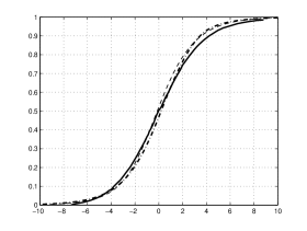
(a) $M_{0}=1.55$

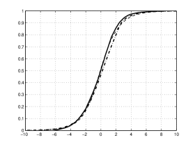
(b) $M_{0}=1.76$

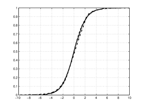
(c) $M_{0}=2.05$

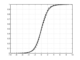
(d) $M_{0}=2.31$

Figure 4: The shock structure for different Mach numbers. All lines are density profiles. The solid lines are the experimental data, and the dashdot lines are R20 results. The thin dashed lines are the results of the discrete velocity model (to be continued).

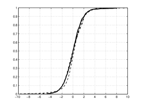
(e) $M_{0}=3.38$

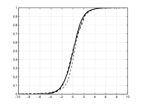
(f) $M_{0}=3.8$

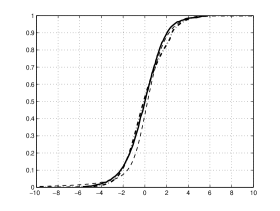
(g) $M_{0}=6.5$

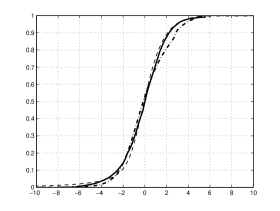
(h) $M_{0}=9.0$

Figure 4: The shock structure for different Mach numbers. All lines are density profiles. The solid lines are the experimental data, and the dashdot lines are R20 results. The thin dashed lines are the results of the discrete velocity model.

As stated in [11], in Grad’s moment theory, a continuous shock structure exists only up to the largest characteristic velocity. For the case of $M=3$, i.e. the 20-moment equations, Weiss [19] has found that no continuous shock is possible when the Mach number is larger than $1.808$. In Figure 4, the moment system with the new regularization produces stable and smooth shock structures for much greater Mach numbers. For $M_{0}<3$, the R20 equations give good agreement with the experimental data, while for larger Mach numbers, the profiles are generally correct, although the predicted density is somewhat lower than the physical case in the high density region.

5 Concluding remarks and discussions

A numerical regularized moment method has been presented. In order to construct the regularization term, we first use Maxwellian iteration to determine the order of magnitude for each moment, and then approximate the high order moments by eliminating terms with small magnitude. Finally, the approximation is greatly simplified by the strategy of linearization. Compared with the regularization in [4], this method not only makes it possible to solve high Mach number flow, but also keeps the convergence to the BGK solution in moment number. Currently, it is still a challenge to get physical shock profiles by this method, and the work on a comprehensive analysis on the shock structure of large moment systems is in progress.

Appendix

Appendix A Some properties of Hermite polynomials

The Hermite polynomials defined in (2.11) are a set of orthogonal polynomials over the domain $(-\infty,+\infty)$. Their properties can be found in many mathematical handbooks such as [1]. Some useful ones are listed below:

1. Orthogonality: $\displaystyle\int_{\mathbb{R}}\mathit{He}_{m}(x)\mathit{He}_{n}(x)\exp(-x^{2}/2)\,\mathrm{d}x=m!\sqrt{2\pi}\delta_{m,n}$;

2. Recursion relation: $\mathit{He}_{n+1}(x)=x\mathit{He}_{n}(x)-n\mathit{He}_{n-1}(x)$;

3. Differential relation: $\mathit{He}_{n}^{\prime}(x)=n\mathit{He}_{n-1}(x)$.

And the following equality can be derived from the last two relations:

$$[\mathit{He}_{n}(x)\exp(-x^{2}/2)]^{\prime}=-\mathit{He}_{n+1}(x)\exp(-x^{2}/2).$$ (A.1)

Appendix B Derivation of the moment equations

In order to derive the analytical form of the moment equations, we need to put the expanded distribution (2.8) into the Boltzmann-BGK equation (2.2). The subsequent calculation will involve the temporal and spatial differentiation of the basis function $\mathcal{H}_{\theta,\alpha}(\boldsymbol{v})$, which will be first calculated as

$$\begin{split}\dfrac{\partial}{\partial{s}}\mathcal{H}_{\theta,\alpha}(\boldsymbol{v})&=-\frac{|\alpha|+D}{2}(2\pi)^{-\frac{D}{2}}\theta^{-\frac{|\alpha|+D}{2}-1}\dfrac{\partial{\theta}}{\partial{s}}\prod_{d=1}^{D}\mathit{He}_{\alpha_{d}}(v_{d})\exp\left(-\frac{v_{d}^{2}}{2}\right)\\ &\quad-(2\pi)^{-\frac{D}{2}}\theta^{-\frac{|\alpha|+D}{2}}\sum_{j=1}^{D}\left[\dfrac{\partial{v_{j}}}{\partial{s}}\prod_{d=1}^{D}\mathit{He}_{\alpha_{d}+\delta_{jd}}(v_{d})\exp\left(-\frac{v_{d}^{2}}{2}\right)\right]\\ &=-\frac{|\alpha|+D}{2\theta}\dfrac{\partial{\theta}}{\partial{s}}\mathcal{H}_{\theta,\alpha}(\boldsymbol{v})-\sqrt{\theta}\sum_{d=1}^{D}\dfrac{\partial{v_{d}}}{\partial{s}}\mathcal{H}_{\theta,\alpha+e_{d}}(\boldsymbol{v}),\end{split}$$ (B.1)

where $s$ stands for $t$ or $x_{j}$, $j=1,2,3$. The partial derivative $\partial v_{d}/\partial s$ can be expanded as

$$\dfrac{\partial{v_{d}}}{\partial{s}}=\dfrac{\partial}{\partial{s}}\left(\frac{\xi_{d}-u_{d}}{\sqrt{\theta}}\right)=-\frac{1}{\sqrt{\theta}}\dfrac{\partial{u_{d}}}{\partial{s}}-\frac{v_{d}}{2\theta}\dfrac{\partial{\theta}}{\partial{s}}.$$ (B.2)

Noting that the recursion of the Hermite polynomials gives

$$v_{d}\mathcal{H}_{\theta,\alpha+e_{d}}(\boldsymbol{v})=\sqrt{\theta}\mathcal{H}_{\theta,\alpha+2e_{d}}(\boldsymbol{v})+\frac{\alpha_{d}+1}{\sqrt{\theta}}\mathcal{H}_{\theta,\alpha}(\boldsymbol{v}),$$ (B.3)

we conclude from (B.1), (B.2) and (B.3) that

$$\dfrac{\partial}{\partial{s}}\mathcal{H}_{\theta,\alpha}(\boldsymbol{v})=\sum_{d=1}^{D}\dfrac{\partial{u_{d}}}{\partial{s}}\mathcal{H}_{\theta,\alpha+e_{d}}(\boldsymbol{v})+\frac{1}{2}\dfrac{\partial{\theta}}{\partial{s}}\sum_{d=1}^{D}\mathcal{H}_{\theta,\alpha+2e_{d}}(\boldsymbol{v}).$$ (B.4)

Replacing $s$ with $t$ in the above equation, one can have the following expansion of the time derivative term in the Boltzmann-BGK equation (2.2) by some simple calculation:

$$\begin{split}\dfrac{\partial{f}}{\partial{t}}&=\sum_{\alpha\in\mathbb{N}^{D}}\left(\dfrac{\partial{f_{\alpha}}}{\partial{t}}\mathcal{H}_{\theta,\alpha}+f_{\alpha}\dfrac{\partial{\mathcal{H}_{\theta,\alpha}}}{\partial{t}}\right)\\ &=\sum_{\alpha\in\mathbb{N}^{D}}\left(\dfrac{\partial{f_{\alpha}}}{\partial{t}}+\sum_{d=1}^{D}\dfrac{\partial{u_{d}}}{\partial{t}}f_{\alpha-e_{d}}+\frac{1}{2}\dfrac{\partial{\theta}}{\partial{t}}\sum_{d=1}^{D}f_{\alpha-2e_{d}}\right)\mathcal{H}_{\theta,\alpha}.\end{split}$$ (B.5)

Now we consider the convection term. Substituting $x_{j}$ for $s$ in (B.4), and making use of (B.3) again, one has

$$\begin{split}\nabla_{\boldsymbol{x}}\cdot(\boldsymbol{\xi}f)&=\sum_{j=1}^{D}\xi_{j}\dfrac{\partial{f}}{\partial{x_{j}}}=\sum_{j=1}^{D}(u_{j}+\sqrt{\theta}v_{j})\sum_{\alpha\in\mathbb{N}^{D}}\left(\dfrac{\partial{f_{\alpha}}}{\partial{x_{j}}}\mathcal{H}_{\theta,\alpha}+f_{\alpha}\dfrac{\partial{\mathcal{H}_{\theta,\alpha}}}{\partial{x_{j}}}\right)\\ &=\sum_{\alpha\in\mathbb{N}^{D}}\mathcal{H}_{\theta,\alpha}\sum_{j=1}^{D}\bigg{[}\left(\theta\dfrac{\partial{f_{\alpha-e_{j}}}}{\partial{x_{j}}}+u_{j}\dfrac{\partial{f_{\alpha}}}{\partial{x_{j}}}+(\alpha_{j}+1)\dfrac{\partial{f_{\alpha+e_{j}}}}{\partial{x_{j}}}\right)\\ &\qquad{}+\sum_{d=1}^{D}\dfrac{\partial{u_{d}}}{\partial{x_{j}}}\left(\theta f_{\alpha-e_{d}-e_{j}}+u_{j}f_{\alpha-e_{d}}+(\alpha_{j}+1)f_{\alpha-e_{d}+e_{j}}\right)\\ &\qquad{}+\frac{1}{2}\dfrac{\partial{\theta}}{\partial{x_{j}}}\sum_{d=1}^{D}\left(\theta f_{\alpha-2e_{d}-e_{j}}+u_{j}f_{\alpha-2e_{d}}+(\alpha_{j}+1)f_{\alpha-2e_{d}+e_{j}}\right)\bigg{]}.\end{split}$$ (B.6)

Using $f_{M}=f_{0}\mathcal{H}_{\theta,0}(\boldsymbol{v})$, the relaxation term can be simply expanded as

$$\frac{1}{\tau}(f_{M}-f)=-\frac{1}{\tau}\sum_{|\alpha|\geqslant 1}f_{\alpha}\mathcal{H}_{\theta,\alpha}(\boldsymbol{v}).$$ (B.7)

Finally, we combine (B.5), (B.6) and (B.7) and find the ultimate moment equations as

$$\begin{split}&\left(\dfrac{\partial{f_{\alpha}}}{\partial{t}}+\sum_{d=1}^{D}\dfrac{\partial{u_{d}}}{\partial{t}}f_{\alpha-e_{d}}+\frac{1}{2}\dfrac{\partial{\theta}}{\partial{t}}\sum_{d=1}^{D}f_{\alpha-2e_{d}}\right)\\ &\qquad+\sum_{j=1}^{D}\bigg{[}\left(\theta\dfrac{\partial{f_{\alpha-e_{j}}}}{\partial{x_{j}}}+u_{j}\dfrac{\partial{f_{\alpha}}}{\partial{x_{j}}}+(\alpha_{j}+1)\dfrac{\partial{f_{\alpha+e_{j}}}}{\partial{x_{j}}}\right)\\ &\qquad{}+\sum_{d=1}^{D}\dfrac{\partial{u_{d}}}{\partial{x_{j}}}\left(\theta f_{\alpha-e_{d}-e_{j}}+u_{j}f_{\alpha-e_{d}}+(\alpha_{j}+1)f_{\alpha-e_{d}+e_{j}}\right)\\ &\qquad{}+\frac{1}{2}\dfrac{\partial{\theta}}{\partial{x_{j}}}\sum_{d=1}^{D}\left(\theta f_{\alpha-2e_{d}-e_{j}}+u_{j}f_{\alpha-2e_{d}}+(\alpha_{j}+1)f_{\alpha-2e_{d}+e_{j}}\right)\bigg{]}=-\frac{1-\delta_{0\alpha}}{\tau}f_{\alpha},\end{split}$$ (B.8)

where $\alpha\in\mathbb{N}^{D}$ and

$$\delta_{0\alpha}=\left\{\begin{array}[]{ll}1,&\alpha=0,\\ 0,&\text{otherwise}.\end{array}\right.$$ (B.9)

References

- [1] M. Abramowitz and I. A. Stegun. Handbook of Mathematical Functions with Formulas, Graphs, and Mathematical Tables. Dover, New York, 1964.
- [2] H. Alsmeyer. Density profiles in argon and nitrogen shock waves measured by the absorption of an electron beam. J. Fluid. Mech., 74(3):497–513, 1976.
- [3] G. A. Bird. Molecular Gas Dynamics and the Direct Simulation of Gas Flows. Oxford: Clarendon Press, 1994.
- [4] Z. Cai and R. Li. Numerical regularized moment method of arbitrary order for Boltzmann-BGK equation. SIAM J. Sci. Comput., 32(5):2875–2907, 2010.
- [5] Z. Cai, R. Li, and Y. Wang. An efficient NR method for Boltzmann-BGK equation. J. Sci. Comput., 2011. DOI: 10.1007/s10915-011-9475-5.
- [6] H. Grad. On the kinetic theory of rarefied gases. Comm. Pure Appl. Math., 2(4):331–407, 1949.
- [7] L. H. Holway. New statistical models for kinetic theory: Methods of construction. Phys. Fluids, 9(1):1658–1673, 1966.
- [8] E. Ikenberry and C. Truesdell. On the pressures and the flux of energy in a gas according to Maxwell’s kinetic theory I. J. Rat. Mech. Anal., 5(1):1–54, 1956.
- [9] L. Mieussens. Discrete velocity model and implicit scheme for the BGK equation of rarefied gas dynamics. Math. Models Methods Appl. Sci., 10(8):1121–1149, 2000.
- [10] I. Müller, D. Reitebuch, and W. Weiss. Extended thermodynamics – consistent in order of magnitude. Continuum Mech. Thermodyn., 15(2):113–146, 2002.
- [11] I. Müller and T. Ruggeri. Rational Extended Thermodynamics, Second Edition, volume 37 of Springer tracts in natural philosophy. Springer-Verlag, New York, 1998.
- [12] E. M. Shakhov. Generalization of the Krook kinetic relaxation equation. Fluid Dyn., 3(5):95–96, 1968.
- [13] H. Struchtrup. Stable transport equations for rarefied gases at high orders in the Knudsen number. Phys. Fluids, 16(11):3921–3934, 2004.
- [14] H. Struchtrup. Derivation of 13 moment equations for rarefied gas flow to second order accuracy for arbitrary interaction potentials. Multiscale Model. Simul., 3(1):221–243, 2005.
- [15] H. Struchtrup. Macroscopic Transport Equations for Rarefied Gas Flows: Approximation Methods in Kinetic Theory. Springer, 2005.
- [16] H. Struchtrup and M. Torrilhon. Regularization of Grad’s 13 moment equations: Derivation and linear analysis. Phys. Fluids, 15(9):2668–2680, 2003.
- [17] M. Torrilhon. Two dimensional bulk microflow simulations based on regularized Grad’s 13-moment equations. SIAM Multiscale Model. Simul., 5(3):695–728, 2006.
- [18] M. Torrilhon. Hyperbolic moment equations in kinetic gas theory based on multi-variate Pearson-IV-distributions. Commun. Comput. Phys., 7(4):639–673, 2010.
- [19] W. Weiss. Continuous shock structure in extended thermodynamics. Phys. Rev. E, 52(6):R5760–R5763, 1995.