Nonlinear effects in resonant layers in solar and space plasmas

Abstract

The present paper reviews recent advances in the theory of nonlinear driven magnetohydrodynamic (MHD) waves in slow and Alfvén resonant layers. Simple estimations show that in the vicinity of resonant positions the amplitude of variables can grow over the threshold where linear descriptions are valid. Using the method of matched asymptotic expansions, governing equations of dynamics inside the dissipative layer and jump conditions across the dissipative layers are derived. These relations are essential when studying the efficiency of resonant absorption. Nonlinearity in dissipative layers can generate new effects, such as mean flows, which can have serious implications on the stability and efficiency of the resonance.

1 Introduction

The dynamical response of the plasma in the solar atmosphere to rapid changes can be manifested through wave propagation along and across the magnetic field. Many of these waves are in the magnetohydrodynamic (MHD) threshold (waves with periods larger than the ion collisional time and wavelengths larger than the mean free path of ions) and they are observable by the new generation of space- and ground-based telescopes in almost all regions of the solar atmosphere (for extensive reviews on wave observation see, e.g., Acton at al., 1981; Nakariakov and Verwichte, 2005; Banerjee et al., 2007).

One of the most fundamental characteristics of solar and space plasmas is their very high degree of inhomogeneity along and across magnetic fields. It is well known that the properties of MHD waves are strongly modified by the plasma inhomogeneity. In particular, when the inhomogeneity of the medium is transversal to the direction of wave propagation a new phenomenon, called resonant absorption, can appear.

While homogenous plasmas have a spectrum of linear eigenmodes which can be divided into slow, fast and Alfvén subspectra, with the slow and fast subspectra having discrete eigenmodes and the subspectrum of Alfvén waves being infinitely degenerated, in inhomogeneous plasmas the three subspectra are substantially changed. According to spectral theories of waves in inhomogeneous plasmas (see, e.g., Goedbloed, 1983; Goedbloed and Poedts, 2004) the spectra of slow and Alfvén waves become continuous while the spectrum corresponding to fast waves becomes discrete. Eigenfunctions that correspond to frequencies in the continuum spectra are improper as they contain a non-square integrable singularity at the resonant position.

According to the accepted resonant wave theories, effective energy transfer between an energy carrying wave and the plasma occurs if the frequency of the wave falls into the slow or Alfvén continuum, i.e. at the slow or Alfvén resonances.

The process of resonant interaction of waves and the possibility of energy transfer between global and local waves has been studied intensively for the past few decades. First resonant absorption was studied as a means of supplementary heating fusion plasmas, but was later rejected due to technical difficulties (see, e.g., Tataronis and Grossman, 1973; Chen and Hasegawa, 1974; Poedts et al., 1989; van Eester et al., 1991).

In the Earth’s magnetosphere resonant MHD wave coupling is believed to generate low frequency pulsation or energize ULF waves (see, e.g. Lanzerotti et al., 1973; Southwood, 1974; Southwood and Hughes, 1983; Ruderman and Wright, 1998; Erdélyi and Taroyan, 2003; Taroyan and Erdélyi, 2002, 2003a, 2003b). Within the context of solar physics Ionson (1978) was the first who proposed resonant absorption as a possible mechanism for coronal heating. His idea was further developed in the last few decades by many authors (see, e.g. Kuperus et al., 1981; Davila, 1987; Hollweg, 1991; Goossens, 1991; Ofman and Davila, 1995; Erdélyi and Goossens, 1994, 1995, 1996; Erdélyi, 1997, 1998; Ballai et al., 2000, etc.), however it became clear soon that resonant absorption alone cannot explain the very high temperature of the corona. Resonant absorption was also used to explain the loss of power in p-modes when interacting with sunspots in the solar photosphere (see, e.g., Hollweg, 1988; Lou, 1990; Goossens and Poedts, 1992; Spruit and Bodgan, 1992; Erdélyi and Goossens, 1994; Keppens et al., 1994; Erdélyi, 1996; Tirry et al., 1998a, b).

Recently resonant absorption acquired a new application in coronal seismology where the rapid damping (with damping times of the order of a few periods) of kink oscillations in coronal loops is explained in terms of resonant interaction of global kink modes and the local Alfvén waves Ruderman and Roberts (2002); Goossens et al. (2002, 2006); Dymova and Ruderman (2006); Erdélyi and Verth (2007); Verth and Erdélyi (2008); Terradas et al. (2010). Coronal seismology is dependent on theoretical relations (dispersion relations) which link plasma parameters, such as the plasma density, to wave parameters, such as the wave frequency, in a precise way. Generally, plasma parameters are determined from wave parameters, which themselves are determined observationally. The dispersion relations for many plasma structures under the assumptions of ideal MHD are well known; they were derived long before accurate EUV observations were available (e.g. Edwin and Roberts, 1983; Roberts et al., 1984) using simplified models within the framework of ideal and linear MHD. Although the realistic interpretation of many observations are made difficult by the spatial and temporal resolution of present satellites not being adequate, considerable amount of information about the state of the plasma and the structure and magnitude of the coronal magnetic field have been already obtained.

At resonance, amplitudes of oscillations (i.e. the energy density) can grow without limits, however even a small amount of dissipation is able to prevent the unlimited increase of the amplitude. The presence of dissipation causes transforming the wave energy into heat. On the other hand solar and space plasmas are media with very high Reynolds numbers (i.e. weakly dissipative media), which means that the dissipation is an important ingredient in the description of dynamics only in a narrow region around the resonant magnetic surfaces called dissipative layer. Outside this layer the dynamics is described by the ideal MHD. This natural structuring of the domain of interest allows us to use the method of matched asymptotic expansions Nayfeh (1981); Bender and Országh (1991) to describe the problem of resonant absorption of MHD waves. The essence of this method resides in solving ideal MHD equations outside the dissipative layer, the non-ideal equations inside the dissipative layer (which contains the resonant surface), and matching the two sets of solutions in overlapping regions (for details see the review by Goossens et al. 2010, this issue).

The dissipation of energies in the solar atmosphere is a delicate problem as the dominance of a certain process over all other possible ones depends on the region where the dynamics will be described and also on the very physics of the problem under consideration. That is why the dynamics of waves in the solar atmosphere is going to be influenced by different dissipation mechanisms in, e.g. the photosphere and solar corona. A full analysis of particular dissipative mechanisms used in the present paper will be given in the next section.

Nonlinearity was systematically overlooked in many studies related to wave dynamics because the mathematical treatment of nonlinear problems is cumbersome, and because the complicated mathematical analysis can often obscure the physics and, therefore, make the results unusable for observers. Dynamics occurring over extended scales (as in the solar atmosphere) are likely to encounter situations which can lead to the increase in amplitudes resulting in breakdown of linear description. Very often the wave amplitudes can increase due to the change of the medium properties, e.g. acoustic waves propagating from the photosphere to the corona can steepen into shocks due to the decrease of the density with height.

A great advantage in tackling the complicated problem of resonant absorption is the notion of connection formulae introduced for the first time by Sakurai et al. (1991). The accuracy of the method by numerics was addressed by Stenuit et al. (1995). This approach assumes that the thin dissipative layer is treated as a surface of discontinuity with the dynamics at both sides of the discontinuity fully described by the ideal MHD. The system of non-ideal MHD equations describing the dynamics inside the dissipative layer is used to obtain the connection formulae that serve as boundary conditions at the surface of discontinuity in the same way as the Rankine-Hugoniot jump conditions for shocks.

A great deal of understanding of the process of resonant absorption came from recent numerical investigations (see, e.g., Ofman at al., 1994; Ofman and Davila, 1995, 1996; Poedts and Goedbloed, 1997), where issues like higher dimension resonance, time evolution of the resonance or randomly driven resonance were discussed in great detail.

The paper is organized as follows. In Section. 2 we introduce the equations used to describe the dynamics of waves and present the mathematical and physical tools employed in the mathematical presentation of the problem. In Section 3 we introduce scalings and dimensionless quantities required to quantify the importance of nonlinearity. The problem of nonlinear slow resonant waves is presented in Section 4, where we describe the nonlinear character of waves near resonance and we provide the jump conditions near the resonance. In Section 5 we show that there are two particular cases where the jump conditions can be simplified into an explicit form. The problem of nonlinear resonant Alfvén waves is discussed in Section 6. As an application to the nonlinear theory reviewed in this paper we will apply the equations to study the efficiency of resonance in the limiting cases of weak and strong nonlinearity. A direct consequence of the nonlinear framework used in our analysis is the generation of mean shear flows at both resonances, which will be presented in Section 8.

2 Basic equations

Solar and space plasmas are far from being an ideal environment with the plasma dynamics being affected by many dissipative and dispersive effects. As stressed earlier, the right choice of dissipative mechanism depends on the location where a particular physical phenomenon takes place as well as on the nature of this phenomenon. For the present paper, we are going to consider viscosity, electrical resistivity and thermal conduction. Dissipative processes are weak in the solar atmosphere; this means that the diffusion coefficients are small. The rate of dissipation, however, is dependent on the local spatial scales.

Many phenomena (e.g. resonant absorption, current sheets or turbulences) are inherently non-ideal and very often nonlinear as they are strongly influenced by dissipative and/or dispersive effects. In particular, dissipation is important for nonlinear dynamical processes because large-scale motions rapidly lead to the formation of small-scale structures, which corresponds to singularities in the ideal theory.

Viscosity and thermal conductivity are linked to hydrodynamical processes, while electrical conductivity and Hall dispersion are related to the presence of the electric and magnetic fields. In the context of solar physics, the general effect of dissipation and dispersion is to relax the accumulation of wave energy in a system. The relaxation can be performed by, e.g. converting the wave energy at resonance into heat by viscous or resistive dissipation or thermal conduction (via resonant absorption), or the dispersion of energy over a larger area by the Hall effect. The relaxation caused by dissipation and dispersion prevents the formation of singularities (entities abhorred by nature).

The key quantities in our discussion are the dimensionless products $\omega_{i}\tau_{i}$ and $\omega_{e}\tau_{e}$, where $\omega_{i(e)}$ is the ion (electron) cyclotron frequency and $\tau_{i(e)}$ is the mean ion (electron) collision time. Since viscosity is mainly due to ions, the product $\omega_{i}\tau_{i}$ is important in describing viscosity. On the other hand, thermal and electrical conductivity are effects attributed mainly to electrons, so the product $\omega_{e}\tau_{e}$ appears in the description of these two dissipative mechanisms.

The classical Braginskii (1965) expression for the viscosity tensor reads

$$\boldsymbol{\mathsf{S}}=\sum_{i=0}^{4}\eta_{i}\boldsymbol{\mathsf{S}}_{i},$$ (1)

where the coefficients $\eta_{0}$, $\eta_{1}$ and $\eta_{2}$ describe viscous damping and $\eta_{3}$ and $\eta_{4}$ are non-dissipative coefficients related to wave dispersion due to the finite ion gyroradius. The quantities $\boldsymbol{\mathsf{S}}_{i}$ are given in terms of the unit vector along the equilibrium magnetic field and the velocity vector. The viscous force in plasmas is given by $\nabla\cdot\boldsymbol{\mathsf{S}}$. In general the expressions for $\eta_{i}$ ($i=1,\dots,4$) and $\boldsymbol{\mathsf{S}}_{i}$ are quite complicated and we do not write them down. The coefficient of compressional viscosity $\eta_{0}$ is given by

$$\eta_{0}\approx\frac{\rho k_{B}T\tau_{i}}{m_{p}},$$ (2)

where $\rho$ and $T$ are the density and temperature of the plasma, $k_{B}$ is the Boltzmann constant and $m_{p}$ is the proton mass. When $\omega_{i}\tau_{i}\ll 1$ as in the solar photosphere, the other coefficients in Eq. (1) are given by

$$\eta_{1}\approx\eta_{2}\approx\eta_{0},\quad\eta_{3}\approx 2\eta_{4}\approx 0.8\eta_{0}(\omega_{i}\tau_{i}).$$ (3)

It can be seen that $\eta_{3},\eta_{4}\ll\eta_{0}$, so that the last two terms in Eq. (1) can be neglected. Then the viscous force is given by the approximate expression

$$\vec{F}_{\rm vis}=\nabla\cdot\boldsymbol{\mathsf{S}}\approx\eta_{0}\big{(}\nabla^{2}\vec{v}+\frac{{}_{1}}{{}^{3}}\nabla\nabla\cdot\vec{v}\big{)},$$ (4)

where $\vec{v}$ is the plasma velocity. This expression for the viscous force is isotropic in the sense that the force is independent of the magnetic field direction.

In the solar chromosphere and, especially in the corona, the condition $\omega_{i}\tau_{i}\gg 1$ is satisfied. In this case the remaining four dissipative coefficients are given by

$$\eta_{1}=\frac{\eta_{0}}{4(\omega_{i}\tau_{i})^{2}}\/,\quad\eta_{2}=4\eta_{1}\/,\quad\eta_{3}=\frac{\eta_{0}}{2\omega_{i}\tau_{i}}\/,\quad\eta_{4}=2\eta_{3}.$$ (5)

Now $\eta_{1},\eta_{2},\eta_{3},\eta_{4}\ll\eta_{0}$, so that, in particular, the compressional viscosity strongly dominates the shear viscosity. As a result all terms in Eq. (1) can be neglected in comparison with the first one, and we arrive at the following approximate expression for the viscous force,

$$\vec{F}_{\rm vis}=\nabla\cdot\boldsymbol{\mathsf{S}}\approx\eta_{0}\nabla\cdot\left(\vec{b}_{0}\otimes\vec{b}_{0}-\frac{{}_{1}}{{}^{3}}\boldsymbol{\mathsf{I}}\right)[3\vec{b}_{0}\cdot(\vec{b}_{0}\cdot\nabla)\vec{v}-\nabla\cdot\vec{v}].$$ (6)

Here $\vec{b}_{0}$ is the unit vector in the magnetic field direction, $\boldsymbol{\mathsf{I}}$ is the unit tensor, and $\vec{f}\otimes\vec{g}$ denotes the dyadic product of vectors $\vec{f}$ and $\vec{g}$.

However, Eq. (6) can be used only in slow dissipative layers. The compressional viscosity is identically zero for Alfvén waves. As a result, it cannot remove the ideal Alfvén singularity Ofman at al. (1994); Erdélyi et al. (1995); Ruderman and Goossens (1996); Mocanu et al. (2008). When studying the motion in Alfvén dissipative layers we have to keep the second and third terms in Eq. (1). On the other hand, in spite that $\eta_{1},\eta_{2}\ll\eta_{0}$, we can neglect the first term in Eq. (1). As for the fourth and fifth terms, they can be neglected because they do not provide dissipation. In addition, we can neglect the spatial variation of the unit vector in the magnetic field direction, $\vec{b}$, in the Alfvén dissipative layer. As a result, we obtain the following expression for the viscous force,

$$\vec{F}_{\rm vis} \approx \eta_{1}\nabla\cdot(\boldsymbol{\mathsf{S}}_{1}+4\boldsymbol{\mathsf{S}}_{2})\approx\eta_{1}\{\nabla^{2}\vec{v}+3\vec{b}_{0}\nabla^{2}(\vec{b}_{0}\cdot\vec{v})+4\vec{b}_{0}\/\/\vec{b}_{0}\cdot\nabla\nabla\cdot\vec{v}$$ (7)

$$+ 3(\vec{b}_{0}\cdot\nabla)[(\vec{b}_{0}\cdot 3\nabla)+\nabla(\vec{b}_{0}\cdot\vec{v})]+\nabla[\vec{b}_{0}\cdot\nabla(\vec{b}_{0}\cdot\vec{v})]$$

$$- 15\vec{b}_{0}\/\/\vec{b}_{0}\cdot\nabla[(\vec{b}_{0}\cdot\nabla(\vec{b}_{0}\cdot\vec{v})]\},$$

which is still rather complicated. However, in Alfvén dissipative layers $\nabla\cdot\vec{v}\approx 0$ which enables us to neglect the third term on the right-hand side of Eq. (7). In addition, in Alfvén dissipative layers large gradients can develop only in the direction perpendicular to the equilibrium magnetic field. This observation enables us to neglect also the fourth, fifth and sixth terms on the right-hand side of Eq. (7). Finally, the dominant component of the velocity in Alfvén dissipative layers is the component orthogonal to the equilibrium magnetic field, while the component along the magnetic field remains small. This means that we can also neglect the second term on the right-hand side of Eq. (7). As a result the very simple expression for the viscous force that can be used in Alfvén dissipative layers is

$$\vec{F}_{\rm vis}\approx\eta_{1}\nabla^{2}\vec{v}.$$ (8)

The wave energy can be also dissipated due to thermal conduction. In what follows we assume that the ions end electrons have equal temperatures. In this case the general expression for the heat flux $\vec{q}$ is given by

$$\vec{q}=-\kappa_{\parallel}\nabla_{\parallel}T-\kappa_{\perp}\nabla_{\perp}T-\kappa_{\wedge}\vec{b}_{0}\times\nabla T,$$ (9)

where $\kappa_{\parallel}$, $\kappa_{\perp}$ and $\kappa_{\wedge}$ are the parallel, perpendicular and skew coefficients of thermal conduction, $\nabla_{\parallel}=\vec{b}_{0}(\vec{b}_{0}\cdot\nabla)$, $\nabla_{\perp}=\nabla-\vec{b}_{0}(\vec{b}_{0}\cdot\nabla)$, and $T$ is the plasma temperature related to the plasma density, $\rho$, and pressure, $p$, by the ideal gas law,

$$p=\frac{k_{B}}{m_{p}}\rho T.$$ (10)

For the electron-proton plasmas, the expression for $\kappa_{\parallel}$ is given by

$$\kappa_{\parallel}\approx\frac{3k_{B}^{2}\rho T\tau_{e}}{m_{p}m_{e}},$$ (11)

where $m_{e}$ is the electron mass. When $\omega_{e}\tau_{e}\ll 1$ as in the lower part of the solar photosphere, $\kappa_{\perp}\approx\kappa_{\parallel}$ and $\kappa_{\wedge}\sim(\omega_{e}\tau_{e})\kappa_{\parallel}\ll\kappa_{\parallel}$. As a result the approximate expression for the heat flux reads

$$\vec{q}=-\kappa_{\parallel}\nabla T.$$ (12)

This expression is isotropic in the sense that it is independent of the magnetic field direction.

When $\omega_{e}\tau_{e}\gg 1$ as in the solar chromosphere and corona, $\kappa_{\perp}\sim(\omega_{e}\tau_{e})^{-2}\kappa_{\parallel}\ll\kappa_{\parallel}$, $\kappa_{\wedge}\sim(\omega_{e}\tau_{e})^{-1}\kappa_{\parallel}\ll\kappa_{\parallel}$, and the first term in Eq. (9) strongly dominates over two other terms. Therefore we can use the approximate expression for the heat flux

$$\vec{q}=-\kappa_{\parallel}\nabla_{\parallel}T.$$ (13)

We now see that the heat flux is in the magnetic field direction, and magnetic surfaces act as thermal insulators.

We write the expression of the generalized Ohm’s equation in the form

$$\vec{E}+\vec{v}\times\vec{B}=\frac{\vec{j}}{\sigma}+\frac{m_{p}}{\rho e}\vec{j}\times\vec{B},$$ (14)

where $e$ is the elementary electrical charge, $\sigma$ the electrical conductivity, $\vec{j}$ the electrical current density, and $\vec{E}$ and $\vec{B}$ are the electric and magnetic field, respectively. The first term on the right-hand side of Eq. (14) is related to the plasma resistivity. It disappears in the limit of infinitely conducting plasmas where $\sigma\to\infty$. The second term on the right-hand side of Eq. (14) describes the Hall current related to the account of the ion inertia. A more general form of the Omh’s equation contains also the term proportional to $\vec{B}\times(\vec{j}\times\vec{B})$ related to the so-called Cowling conductivity (see, e.g. Priest 2000). This term is identically zero for a fully ionized plasma, while in partially ionized plasmas, can be important only when the electron gyrofrequency is large and the plasma is sufficiently rarified, so that the mean collision time between electrons and neutrals is large. On this ground we disregard this term. In what follows we neglect the displacement current in Maxwell’s equations and use Ampere’s law to relate the electrical current density and magnetic field,

$$\mu_{0}\vec{j}=\nabla\times\vec{B},$$ (15)

where $\mu_{0}$ is permeability of free space.

In our analysis we use the system of MHD equations

$$\frac{\partial\rho}{\partial t}+\nabla\cdot{\rho\vec{v}}=0,$$ (16a)

$$\rho\left(\frac{\partial\vec{v}}{\partial t}+\vec{v}\cdot\nabla\vec{v}\right)=-\nabla p+\frac{1}{\mu_{0}}(\nabla\times\vec{B})\times\vec{B}+\vec{F}_{\rm vis},$$ (16b)

$$\frac{\partial\vec{B}}{\partial t}=-\nabla\times\vec{E},$$ (16c)

$$\frac{\partial}{\partial t}\left(\frac{p}{\rho^{\gamma}}\right)+\vec{v}\cdot\nabla\left(\frac{p}{\rho^{\gamma}}\right)=-\frac{\gamma-1}{\rho^{\gamma}}{\cal L}.$$ (16d)

In these equations $\vec{F}_{\rm vis}$ is given either by Eq. (4), Eq. (6) or Eq. (8), and $\vec{E}$ is given by Eq. (14); $\gamma$ is the ratio of specific heats or adiabatic index, and ${\cal L}$ is the loss function given by

$${\cal L}=\nabla\cdot\vec{v}-\frac{\vec{j}^{2}}{\sigma}-\boldsymbol{\mathsf{S}}:\nabla\vec{v},$$ (17)

where $\boldsymbol{\mathsf{S}}$ is the viscosity tensor and the colon indicates the double summation,

$$\boldsymbol{\mathsf{S}}:\nabla\vec{v}=S_{ij}\frac{\partial v_{i}}{\partial x_{j}}.$$ (18)

Recall that the magnetic field is solenoidal, i.e.

$$\nabla\cdot\vec{B}=0.$$ (19)

This equation can be considered as an initial condition imposed on the magnetic field because, if it is satisfied at $t=0$, then it follows from Eq. (16c) that it is satisfied for any $t>0$. If we neglect the Hall term in Eq. (14) then the induction equation (16c) reduces to

$$\frac{\partial\vec{B}}{\partial t}=\nabla\times(\vec{v}\times\vec{B})+\eta\nabla^{2}\vec{B},$$ (20)

where $\eta=1/\mu_{0}\sigma$ is the coefficient of magnetic diffusion. These equations must be supplemented by the Ohm’s law (14) expressing the connection between the electric field and magnetic field.

3 General discussion and dimensionless parameters

Traditionally the importance of dissipative processes in MHD is characterized by dimensionless parameters calculated as ratio of corresponding dissipative terms to dynamical terms. The importance of viscosity is quantified by the viscous Reynolds number. In the previous section we have seen that the coefficients of compressional and shear viscosity can be quite different, so that we have to introduce two Reynolds number, one related to compressional and another to shear viscosity,

$$R_{e}^{c}=\frac{\rho_{*}VL}{\eta_{0}},\qquad R_{e}^{s}=\frac{\rho_{*}VL}{\eta_{1}},$$ (21)

where $V$ is a characteristic speed, usually taken to be equal to the phase speed of waves, $L$ a characteristic length, and $\rho_{*}$ a characteristic density. Of course, where the viscosity is isotropic, $R_{e}^{c}=R_{e}^{s}=R_{e}$ and $\vec{F}_{\rm vis}$ is given by Eq. (4). The characteristic length $L$ plays a very important role in Eq. (21). Far from resonant layers it can be taken to be equal to the wave length. Typically in the solar corona we obtain very large values of $R_{e}^{c}$ and $R_{e}^{s}$, which enables us to neglect viscosity, for example, $R_{e}^{s}=10^{3}\div 10^{4}$ and $R_{e}^{s}=10^{12}\div 10^{14}$.

The importance of resistivity is characterised by the magnetic Reynolds number defined as

$$R_{m}=\frac{VL}{\eta}.$$ (22)

For the solar corona typically $R_{m}=10^{12}\div 10^{14}$.

Finally, the importance of thermal conduction is characterised by the Péclet number which is given by

$$P_{e}=\frac{k_{B}\rho_{*}VL}{m_{p}\kappa_{\parallel}}.$$ (23)

This number is very large in the solar photosphere ($10^{8}-10^{9}$), but it can be of the order of 100 in the solar corona.

The situation with the resistivity and thermal conduction is similar to that of viscosity. Usually we can neglect them far from dissipative layers and consider plasmas as infinitely conducting ($\sigma\to\infty)$ and their motions as adiabatic. However, these two dissipative processes can be again very important inside the dissipative layer.

Linear theory predicts the existence of slow and Alfvén dissipative layers (e.g. Goossens et al., 2010). When the dominant dissipative processes are the isotropic plasma viscosity and resistivity, as in the solar photosphere, it is convenient to introduce the total isotropic Reynolds number, $R_{i}$, defined by

$$\frac{1}{R_{i}}=\frac{1}{R_{e}}+\frac{1}{R_{m}}.$$ (24)

Let us also introduce the dimensionless wave amplitude far from a dissipative layer, $\epsilon\ll 1$. Then linear theory predicts that the amplitudes of perturbations of certain variables called ‘large variables’ in a slow dissipative layer embracing the slow resonant position are of the order of $\epsilon R_{i}^{1/3}$. The linear theory can be used to describe the motion in the slow dissipative layer only when dissipation in this layer strongly dominates over nonlinearity. Estimates show that the ratio of the largest typical nonlinear term in the MHD equations to the largest dissipative term is of the order of (see, e.g. Ruderman et al. 1997a)

$$N_{i}=\epsilon R_{i}^{2/3}.$$ (25)

The linear description is only valid when $N_{i}\ll 1$. In the solar photosphere, however, $\epsilon=10^{-2}\div 10^{-3}$ and $R_{i}\gtrsim 10^{6}$, so that $N_{i}\gtrsim 10$. This estimate clearly shows that the motion in slow dissipative layers is strongly nonlinear in the solar photosphere.

In the solar corona the dominant dissipative processes affecting slow waves are the compressional viscosity and thermal conduction (recall that it is strongly anisotropic and the heat flux is parallel to the magnetic field). To characterise both dissipative processes simultaneously we introduce the total anisotropic Reynolds number defined by (see, e.g. Ballai et al. 1998a)

$$\frac{1}{R_{a}}=\frac{1}{R_{e}^{c}}+\frac{1}{P_{e}}.$$ (26)

The linear theory predicts that the amplitude of large variables in dissipative layers is of the order of $\epsilon R_{a}$, while the ratio of the largest nonlinear term in the MHD equations to the largest dissipative term is of the order of

$$N_{a}=\epsilon R_{a}^{2}.$$ (27)

Again, the linear description is only valid when $N_{a}\ll 1$. In the solar corona for a typical $\epsilon=10^{-2}\div 10^{-3}$ and $R_{a}\gtrsim 100$, so we obtain $N_{a}\gtrsim 10$, and the motion in slow dissipative layers in the solar corona is strongly nonlinear.

Viscosity and resistivity are also the dominant dissipative processes in Alfvén dissipative layer in the solar photosphere. Hence their importance can be characterized by $R_{i}$. Since the quasi-Alfvénic motion in Alfvén dissipative layers practically do not perturb the plasma temperature, thermal conduction is not important in these layers. Since, in addition, compressional viscosity also does not operate in Alfvén dissipative layers, the dominant dissipative processes in these layers in plasmas with strongly anisotropic viscosity like in the solar corona are the shear viscosity and resistivity. These two processes can be simultaneously described by the total Alfvén Reynolds number $R_{A}$ defined by an equation similar to Eq. (24) but with $R_{e}^{s}$ substituted for $R_{e}$. Applying the same formal procedure as that resulted in Eq. (25) we obtain a similar estimate for the ratio of the typical largest nonlinear term in the MHD equations to the largest dissipative term $N_{A}$. On the basis of this estimate we conclude that the linear description of Alfvén dissipative layers breaks down as soon as $\epsilon\gtrsim R_{A}^{-2/3}$. However, as it will be explain later, this conclusion is wrong as in Alfvén dissipative layers the largest nonlinear terms in the MHD equations cancel each other.

4 Governing equation for motion in slow dissipative layers

In what follows we adopt Cartesian coordinates $x,\,y,\,z$ and assume that the equilibrium quantities depend on $x$ only, while the equilibrium magnetic field is unidirectional and parallel to the $yz$-plane. In the equilibrium plasma is at rest. We only consider a two-dimensional problem and assume that perturbations of all quantities are independent of $y$.

In order to derive the equation governing the wave motion inside slow dissipative layers we need to use the matching conditions with the solution of linear ideal MHD equations outside the dissipative layer, which we will call the external solution. Hence, before we embark on the derivation of the governing equation for slow dissipative layer we briefly discuss this external solutions.

To obtain the external solution we write all variables in the system of MHD equations as a sum of an equilibrium quantity and their Eulerian perturbation

$$p=p_{0}+p^{\prime},\quad\rho=\rho_{0}+\rho^{\prime},\quad\vec{B}=\vec{B}_{0}+\vec{b}.$$ (28)

We substitute these expressions in the ideal MHD equations and linearize them with respect to perturbations. We Fourier-analyse the obtained linear equations with respect to $z$ and $t$ and take all quantities proportional to $\exp(ikz-i\omega t)$. Finally, we eliminate all the variables from these equations in favour of the $x$-component of velocity, $u$, and the total pressure perturbation $P=p^{\prime}+\vec{B}_{0}\cdot\vec{b}/\mu_{0}$ to obtain the system of two first-order ordinary differential equations of the form

$$\frac{du}{dx}=\frac{i\omega P}{F},\qquad\frac{dP}{dx}=\frac{ik\rho_{0}D_{A}u}{V}.$$ (29)

In these equations $V=\omega/k$ is the phase velocity and

$$F=\frac{\rho_{0}D_{A}D_{C}}{V^{4}-V^{2}(v_{A}^{2}+c_{S}^{2})+v_{A}^{2}c_{S}^{2}\cos^{2}\alpha},$$ (30)

$$D_{A}=V^{2}-v_{A}^{2}\cos^{2}\alpha,\quad D_{C}=(v_{A}^{2}+c_{S}^{2})(V^{2}-c_{T}^{2}\cos^{2}\alpha),$$ (31)

where the Alfvén $v_{A}$, the sound $c_{S}$, and cusp $c_{T}$, speeds are defined as

$$v_{A}^{2}=\frac{B_{0}^{2}}{\mu_{0}\rho_{0}},\quad c_{S}^{2}=\frac{\gamma p_{0}}{\rho_{0}},\quad c_{T}^{2}=\frac{v_{A}^{2}c_{S}^{2}}{v_{A}^{2}+c_{S}^{2}},$$ (32)

with $\alpha$ being the angle between $\vec{B}_{0}$ and the $z$-axis, i.e. $\cos\alpha=B_{0z}/B_{0}$.

The system of equations (29) has two regular singular points, $x_{A}$ and $x_{c}$. The first point is defined by the equation $D_{A}(x_{A})=0$ and corresponds to the Alfvén resonance. The second point is defined by the equation $D_{C}(x_{c})=0$ and corresponds to the slow or cusp resonance. Using the Fröbenius expansions one can show that the asymptotic behaviour of solution in the vicinity of these points is given by $P\sim\mbox{const}$ and $u\sim\mbox{const}\times\ln|x-x_{A,c}|$. Hence, $P$ is a regular function in the vicinity of the Alfvén and slow singularity. The asymptotic behaviour of other quantities can be determined from the linearized MHD equations. Hence, in the vicinity of the Alfvén resonance, this behaviour is given by (see, e.g. Sakurai et al. 1991; Ofman et al. 1994; Erdélyi and Goossens 1995; Erdélyi 1997, 1998)

$$\begin{array}[]{lll}\displaystyle u\sim\mbox{const}\times\ln|x-x_{A}|,&v_{\parallel}\sim\mbox{const},&\displaystyle v_{\perp}\sim\frac{\mbox{const}}{x-x_{A}},\vspace*{1mm}\\ \displaystyle b_{x}\sim\mbox{const}\times\ln|x-x_{A}|,&b_{\parallel}\sim\mbox{const},&\displaystyle b_{\perp}\sim\frac{\mbox{const}}{x-x_{A}},\vspace*{1mm}\\ \rho^{\prime}\sim\mbox{const},&p^{\prime}\sim\mbox{const},&P\sim\mbox{const},\end{array}$$ (33)

where $v_{\parallel}$ is the velocity component parallel to the equilibrium magnetic field, and $v_{\perp}$ is the velocity component perpendicular both to the equilibrium magnetic field and to the $x$-direction. These two quantities are defined by

$$v_{\parallel}=\vec{v}\cdot\vec{B}_{0}/B_{0},\qquad v_{\perp}=\vec{v}\cdot(\vec{B}_{0}\times\vec{e}_{x})/B_{0},$$ (34)

where $\vec{e}_{x}$ is the unit vector in the $x$-direction. The quantities $b_{\parallel}$ and $b_{\perp}$ can be determined in a similar way. The asymptotic behaviour of perturbations at slow resonance are (see, e.g. Sakurai et al. 1991; Ballai et al. 2000a)

$$\begin{array}[]{lll}\displaystyle u\sim\mbox{const}\times\ln|x-x_{c}|,&\displaystyle v_{\parallel}\sim\frac{\mbox{const}}{x-x_{c}},&v_{\perp}\sim\mbox{const},\vspace*{1mm}\\ \displaystyle b_{x}\sim\mbox{const}\times\ln|x-x_{c}|,&\displaystyle b_{\parallel}\sim\frac{\mbox{const}}{x-x_{c}},&b_{\perp}\sim\mbox{const},\vspace*{1mm}\\ \displaystyle\rho^{\prime}\sim\frac{\mbox{const}}{x-x_{c}},&\displaystyle p^{\prime}\sim\frac{\mbox{const}}{x-x_{c}},&P\sim\mbox{const}.\end{array}$$ (35)

The obvious result of Eq. (33) is that the most singular variables at $x=x_{A}$ are $v_{\perp}$ and $b_{\perp}$ and here they have a $1/x$ singularity. Due to their behaviour at the resonant position they are called the large variables. In accordance with Eq. (35), the large variables at the slow resonant position $x_{c}$ are $v_{\parallel}$, $b_{\parallel}$, $\rho^{\prime}$ and $p^{\prime}$.

An important consequence of Eqs. (33) and (35) is that the perturbation of the total pressure, $P$, does not change across the dissipative layer. The physical reason for this behaviour resides in the fact that since the dissipative layer is thin, i.e. its inertia is very small, the acceleration of the dissipative layer is finite, the total force applied to it has to be small. This implies that the total pressure at the two sides of the dissipative layer has to be almost the same. If we denote the thickness of the dissipative layer as $\ell$ and the characteristic length of the problem as $L$, then the variation of the total pressure across the dissipative layer is zero in the zero-order approximation with respect to the small parameter $\ell/L$. The conclusion that there is no jump of total pressure perturbation across the dissipative layer is obtained here on the basis of ideal MHD. This conclusion is confirmed by the linear theory of dissipative layers based on dissipative MHD (e.g. Goossens et al. 1995 for Alfvén resonance and Erdélyi 1997 for slow resonance).

The linear theory suggests the following physical picture of wave motion in slow dissipative layers. The global motion of the plasma is in exact resonance with slow waves at the ideal resonant position, and it is in quasi-resonance with slow waves in a narrow dissipative layer embracing the resonant position. The variation of the external total pressure acts as a driver of slow waves in the dissipative layer. Hence, the aim of nonlinear theory is to derive the equation governing the nonlinear evolution of slow waves in the dissipative layer.

Ruderman et al. (1997a) were the first who considered this problem. In their analysis they assumed that the only dissipative processes operating in the plasma are resistivity and isotropic viscosity, and both dissipative processes are weak, i.e. dissipation is characterized by $R_{i}\gg 1$. They considered the motion in the form of a propagating wave with permanent shape, so that perturbations of all variables depend on the linear combination $\theta=z-Vt$ rather than $z$ and $t$ separately. The phase speed of slow waves at $x_{c}$ is equal $c_{Tc}\cos\alpha$, where the subscript ‘$c$’ indicates that a quantity is calculated at $x=x_{c}$, so $V=c_{Tc}\cos\alpha$. Finally, Ruderman et al. (1997a) assumed that perturbations of all variables are periodic with respect to $\theta$ with the period (wave length) equal to $L$. Later Ruderman and Erdélyi (2000) generalized this derivation to allow slow time variation of the wave shape, so that perturbations of all variables are functions of $x$, $\theta$ and ‘slow’ time $\tau$. In what follows we briefly outline this derivation.

To obtain the governing equation that simultaneously describes both nonlinear and dissipative effects we formally take $N_{i}\sim 1$, so that $R_{i}\sim\epsilon^{-3/2}$. This assumption is formal in the sense that one can consider $N_{i}\ll 1$, in which case we can neglect nonlinearity in comparison with dissipation, and $N_{i}\ll 1$, in which case we can neglect dissipation in comparison with nonlinearity. Linear theory predicts that the characteristic thickness of the dissipative layer is $LR_{i}^{1/3}\sim\epsilon^{1/2}$. This implies that it is convenient to introduce the stretching variable $\xi=\epsilon^{-1/2}(x-x_{c})$ in the dissipative layer. It is also practical to introduce the ‘slow’ time $\tau=\epsilon^{1/2}t$.

The nonlinear interaction of the wave motion in the dissipative layer with the plasma causes the mean flow in the $yz$-plane with the amplitude of the order of $\epsilon^{1/2}$. Hence, it is convenient to split the velocity components in the mean and oscillating parts,

$$v_{\parallel}=\bar{v}_{\parallel}+\tilde{v}_{\parallel},\quad v_{\perp}=\bar{v}_{\perp}+\tilde{v}_{\perp},\quad\bar{v}_{\parallel}=\langle v_{\parallel}\rangle,\quad\bar{v}_{\perp}=\langle v_{\perp}\rangle,$$ (36)

where the mean value of a period function $f(\theta)$ over the period is defined by

$$\langle f(\theta)\rangle=\frac{1}{L}\int_{0}^{L}f(\theta)\,d\theta.$$

It follows from Eq. (35) that, in the dissipative layer, $v_{\parallel}\sim\epsilon^{1/2}$, $b_{\parallel}\sim\epsilon^{1/2}$, $\rho^{\prime}\sim\epsilon^{1/2}$, $p^{\prime}\sim\epsilon^{1/2}$, $u\sim\epsilon\ln\epsilon$, $b_{x}\sim\epsilon\ln\epsilon$, $v_{\perp}\sim\epsilon$, $b_{\perp}\sim\epsilon$, and $P\sim\epsilon$. Since $|\ln\epsilon|$ is much smaller than any negative power of $\epsilon$ for $\epsilon\ll 1$, in what follows we consider $\ln\epsilon$ as a quantity of the order of unity and we look for the solution to the dissipative MHD equations in the form of power series expansions with respect to $\epsilon^{1/2}$. We write this expansions in the form $f=\epsilon^{1/2}f_{1}+\epsilon f_{2}+\dots$ for $p^{\prime}$, $\rho^{\prime}$, $\tilde{v}_{\parallel}$, $b_{\parallel}$, $\bar{v}_{\parallel}$ and $\bar{v}_{\perp}$, and in the form $g=\epsilon g_{1}+\epsilon^{3/2}g_{2}+\dots$ for $u$, $\tilde{v}_{\perp}$, $b_{x}$, $b_{\perp}$ and $P$.

Substituting the power series expansions in the dissipative MHD equation we obtain in the first order approximation a solution that recovers the results of the linear theory. The compatibility condition for the equations of the second order approximation gives the governing equation for the wave motion in the slow dissipative layer,

$$2\frac{\partial\tilde{v}_{\parallel}}{\partial t}-\frac{\Delta_{c}(x-x_{c})}{V}\frac{\partial\tilde{v}_{\parallel}}{\partial\theta}+\Lambda\tilde{v}_{\parallel}\frac{\partial\tilde{v}_{\parallel}}{\partial\theta}-\lambda_{i}\frac{\partial^{2}\tilde{v}_{\parallel}}{\partial x^{2}}=-\frac{c_{Tc}^{2}\cos\alpha}{\rho_{0c}v_{Ac}^{2}}\frac{dP}{d\theta},$$ (37)

where

$$\Delta_{c}=\left.\frac{d}{dx}(V^{2}-c_{T}^{2}\cos^{2}\alpha)\right|_{x=x_{c}},$$ (38)

$$\Lambda=\frac{v_{Ac}^{2}[(\gamma+1)v_{Ac}^{2}+3c_{Sc}^{2}]\cos\alpha}{(v_{Ac}^{2}+c_{Sc}^{2})^{2}},\quad\lambda_{i}=\frac{\eta_{0}}{\rho_{0c}}+\frac{c_{Tc}^{2}\eta}{v_{Ac}^{2}}.$$ (39)

When deriving Eq. (37) we considered that $\tilde{v}_{\parallel}\approx\epsilon^{1/2}\tilde{v}_{\parallel 1}$. In Eq. (37) $P$ is considered as a given function and it is determined by the solution to the linear ideal MHD equations outside the dissipative layer.

As we have already mentioned, the main idea of connection formulae is to consider the dissipative layer as a surface of discontinuity and use the expressions for the jumps of $P$ and $u$ across the dissipative layer as the boundary conditions for the system of equations (29). The jump of total pressure is the same as in linear theory (see, e.g., Hollweg, 1988; Sakurai et al., 1991; Goossens and Ruderman, 1995; Ruderman and Goossens, 1996),

$$[P]=0,$$ (40)

where, in general, the jump of a function $f$ across the dissipative layer is defined by

$$[f]=\lim_{\xi\to\infty}\{f(\xi)-f(-\xi)\}.$$

(recall that $\xi=\epsilon^{-1/2}(x-x_{c})$). To calculate the expression of $[u]$ we use the relation between $u$ and $\tilde{v}_{\parallel}$ obtained in the first order approximation in the process of derivation of Eq. (37), i.e.

$$\frac{\partial u}{\partial x}+\frac{c_{Tc}^{2}\cos\alpha}{v_{Ac}^{2}}\frac{\partial w}{\partial\theta}=0,$$ (41)

where we have assumed $u\approx\epsilon u_{1}$ and $\tilde{v}_{\parallel}\approx\epsilon^{1/2}\tilde{v}_{\parallel 1}$. It immediately follows from Eq. (41) that

$$[u]=-\frac{c_{Tc}^{2}\cos\alpha}{v_{Ac}^{2}}{\cal P}\int_{-\infty}^{\infty}\frac{\partial\tilde{v}_{\parallel}}{\partial\theta}\,dx.$$ (42)

In the above equation $\cal P$, denotes the Cauchy principal part of the integral which is used since $\tilde{v}_{\parallel}\sim x^{-1}$ as $x\to\infty$, so that the integral in Eq. (41) is divergent.

In linear theory the jump in the normal component of velocity, $[u]$, can be obtained explicitly in terms of $P$. In contrast, in the nonlinear theory we, in general, cannot solve Eq. (37) analytically and obtain an explicit expression for $[u]$, which makes the connection formulae perhaps less practical. However we will see in Sect. 5 that there is one exception.

Ballai et al. (1998a) extended the derivation by Ruderman et al. (1997a) where the dominant dissipation processes are compressional viscosity and thermal conduction along the magnetic field lines. They formally assumed that $N_{a}\sim 1$, so that $R_{a}\sim\epsilon^{-1/2}$. Only the motion periodic with respect to $\theta$ has been considered. Using the same procedure as one adopted by Ruderman et al. (1997a), Ballai et al. (1998a) obtained that the governing equation for the motion in slow dissipative layers is

$$\frac{\Delta_{c}(x-x_{c})}{V}\frac{\partial\tilde{v}_{\parallel}}{\partial\theta}-\Lambda\tilde{v}_{\parallel}\frac{\partial\tilde{v}_{\parallel}}{\partial\theta}+\lambda_{a}\frac{\partial^{2}\tilde{v}_{\parallel}}{\partial\theta^{2}}=\frac{c_{Tc}^{2}\cos\alpha}{\rho_{0c}v_{Ac}^{2}}\frac{dP}{d\theta},$$ (43)

where now

$$\lambda_{a}=\frac{\eta_{0}V^{2}(2v_{Ac}^{2}+3c_{Sc}^{2})^{2}}{3\rho_{c}v_{Ac}^{2}c_{Sc}^{2}(v_{Ac}^{2}+c_{Sc}^{2})}+\frac{(\gamma-1)^{2}m_{p}\kappa_{\parallel}V^{2}}{\gamma\rho_{0c}k_{B}c_{Sc}^{2}}.$$ (44)

The main difference between Eq. (44) and Eq. (37) is in the terms describing the effect of dissipation, which is the last term on the right-hand side of Eq. (44), where it is proportional to the second derivative with respect to $\theta$, while in Eq. (37) the corresponding term is proportional to the second derivative with respect to $x$. Another difference is that Eq. (44) does not contain the derivative with respect to time. This is related to the fact that Ballai et al. (1998a) did not allow slow time variation of the wave shape in the dissipative layer. The extension of the derivation to include this effect is straightforward.

The derivation of governing equations for wave motion in slow dissipative layers has been extended to include the effect of steady flow Ballai and Erdélyi (1998), cylindrical equilibrium Ballai et al. (2000) and the twist of magnetic field lines Ballai and Erdélyi (2002); Erdélyi and Ballai (2002).

Recently, Clack and Ballai (2008) generalized the derivation of governing equation for the wave motion in slow dissipative layers in order to take the Hall effect into account. The ratio of the second term on the right-hand side of the generalized Ohm’s equation (14) describing the Hall effect to the first term describing the plasma resistivity is of the order of $\omega_{e}\tau_{e}$. In the solar corona typically $\omega_{e}\tau_{e}\gtrsim 10^{6}$, so that the Hall term strongly dominates over the resistive term. In classical MHD the magnetic field is frozen in the plasma when the plasma is infinitely conducting. When the Hall term is taken into account the magnetic field is frozen in the electronic component of an infinitely conducting plasma, while the ions can drift with respect to the magnetic field lines. Hence, the account of the Hall term is equivalent to the account of ion inertia. The MHD theory where the Hall effect is taken into account is called the Hall MHD.

Clack and Ballai (2008) repeated the derivation carried out by Ballai et al. (1998a) however in the framework of the Hall MHD. As a result they obtained that the dynamics of waves inside the dissipative layer is given by

$$\frac{\Delta_{c}(x-x_{c})}{V}\frac{\partial\tilde{v}_{\parallel}}{\partial\theta}-\Lambda\tilde{v}_{\parallel}\frac{\partial\tilde{v}_{\parallel}}{\partial\theta}+\lambda_{a}\frac{\partial^{2}\tilde{v}_{\parallel}}{\partial\theta^{2}}+h_{a}\frac{\partial\tilde{v}_{\parallel}}{\partial x}\frac{\partial\tilde{v}_{\parallel}}{\partial\theta}=\frac{c_{Tc}^{2}\cos\alpha}{\rho_{0c}v_{Ac}^{2}}\frac{dP}{d\theta},$$ (45)

where

$$h_{a}=\frac{\eta(\omega_{e}\tau_{e})k^{2}V\tan\alpha}{c_{Sc}^{2}+v_{Ac}^{2}}.$$ (46)

In case when the dominant dissipative processes are the compressional viscosity and thermal conduction the characteristic thickness of slow dissipative layers given by the linear theory is

$$\delta_{c}^{a}=\frac{kV\lambda_{a}}{|\Delta_{c}|}.$$ (47)

This result is easily obtained assuming that the first and third terms in Eq. (45) are of the same order. Using Eq. (47) we obtain that the ratio of the second nonlinear term proportional to $h_{a}$ in Eq. (45) to the first nonlinear term proportional to $\Lambda$ is of the order of

$$\frac{\beta(\omega_{e}\tau_{e})}{R_{m}}\left(\frac{\beta}{R_{e}^{c}}+\frac{1}{P_{e}}\right)^{-1},$$

where the plasma-beta is defined by $\beta=c_{Sc}^{2}/v_{Ac}^{2}$. In particular, in the corona, where $\beta\lesssim 0.01$, $P_{e}\sim 100<R_{e}^{c}$, $R_{m}=10^{12}\div 10^{14}$ and $\omega_{e}\tau_{e}\sim 10^{7}$, this ratio does not exceed $10^{-5}$. Probably, it can be more pronounced in the chromosphere where $\omega_{e}\tau_{e}$ is already quite large, but $R_{m}$ is much smaller than in the corona.

5 Explicit connection formulae

As we have seen in the previous subsection, in general, the first connection formula, which expresses the continuity of the total pressure, is given in the explicit form no matter what is the value of the nonlinearity parameter in a slow dissipative layer (see Eq. (40)). In contrast, we cannot write down an explicit expression for the jump of the normal component of velocity $[u]$ , in general. Instead, to find $[u]$, we first need to solve the governing equation for $\tilde{v}_{\parallel}$, then substitute $\tilde{v}_{\parallel}$ in Eq. (42) and calculate the integral in this equation. As a result, we cannot separate solutions in the resonant layer and in the external regions. Instead, we have to solve the linear ideal MHD equations in the external regions and the governing equation for $\tilde{v}_{\parallel}$ in the dissipative layer simultaneously using the connection formulae Eqs. (40) and (42) to connect the solutions. This makes solving any problem involving nonlinear slow resonance quite complicated.

However, there are two exceptions when we can obtain the second connection formula in an explicit form. The first one is the linear theory. In this case the connection formulae for the cylindrical geometry have been derived by Erdélyi et al. (1995). These formulae are easily translated to the planar geometry. We do not give these formulae here because our aim is to study nonlinear effects in dissipative layer, but refer to Goossens et al. (2010) in this volume.

The second exceptional case is the limit of very strong nonlinearity, when nonlinearity in a slow dissipative layer strongly dominates over dissipation ($N_{i}\gg 1$ or $N_{a}\gg 1$). In this case the explicit expression for $[u]$ has been derived by Ruderman (2000). In what follows we briefly outline the derivation of this expression and the main points. Note that Ruderman (2000) assumed that the equilibrium magnetic field is in the $z$-direction. Here we consider the general case when the equilibrium magnetic field has both $y$ and $z$-component, the angle between the $z$-axis and the equilibrium magnetic field being $\alpha$.

In what follows we consider that the dominant dissipative processes are the isotropic viscosity and plasma resistivity. We assume that the motion is periodic with respect to the coordinate $z$. so that the wave motion in the dissipative layer is described by Eq. (37) with the time derivative equal to zero. Let us introduce the modified nonlinearity parameter

$$N=\epsilon^{3/2}(kx_{0})^{2}R_{i},$$ (48)

where $x_{0}$ is the characteristic spatial scale of inhomogeneity, $k=2\pi/L$, and $L$ is the period with respect to $z$. The condition that nonlinearity dominates over dissipation in the dissipative layer is written as $N\gg 1$. Let us introduce the dimensionless variables

$$\vartheta=k\theta,\;\;\sigma=-\frac{(x-x_{c})\mbox{sign}(\Delta_{c})}{\delta_{c}(2N)^{1/3}},\;\;q=\frac{V\Lambda\tilde{v}_{\parallel}}{\delta_{c}|\Delta_{c}|(2N)^{1/3}},\;\;Q=\frac{2c_{Tc}^{3}\Lambda P\cos^{2}\alpha}{\rho_{0c}v_{Ac}^{2}|\Delta_{c}|\delta_{c}(2N)^{2/3}},$$ (49)

where

$$\delta_{c}=\left[\frac{V}{k|\Delta_{c}|}\left(\frac{\eta_{0}}{\rho_{0c}}+\frac{c_{Tc}^{2}}{v_{Ac}^{2}}\eta\right)\right]^{1/3}$$ (50)

is the characteristic thickness of slow dissipative layer given by the linear theory. In the new variables Eq. (37) with $\partial\tilde{v}_{\parallel}/\partial t=0$ is rewritten as

$$2\sigma\frac{\partial q}{\partial\vartheta}+2q\frac{\partial q}{\partial\vartheta}-\frac{1}{N}\frac{\partial^{2}q}{\sigma^{2}}=-\frac{dQ}{d\vartheta}.$$ (51)

Now $q$ is a periodic function of $\vartheta$ with the period $2\pi$. Since $\langle\tilde{v}_{\parallel}\rangle=0$ it follows $\langle q\rangle=0$. It is easy to see that this restriction on $q$ is compatible with Eq. (51). Let us look for the solution to Eq. (51) satisfying this condition in the form of asymptotic expansion with respect to the small parameter $1/N$,

$$q=\sum_{n=0}^{\infty}N^{-n}q^{(n)}.$$ (52)

Let us assume that the function $Q(\vartheta)$ (and, consequently, $P(\vartheta)$) takes its maximum value in the interval $[0,2\pi]$ at exactly one point $\vartheta_{M}$. We denote this value as $Q_{M}$ and the maximum value of $P$ as $P_{M}$. This assumption implies that $Q(\vartheta_{M}+2\pi n)=Q_{M}$, and $Q(\vartheta)<Q_{M}$ when $\vartheta\neq\vartheta_{M}+2\pi n$, where $n$ is any integer number. Ruderman (2000) has shown that, under this condition, there is a quantity $\sigma_{0}>0$ so that the function $q^{(0)}$ can be written as

$$q^{(0)}=\left\{\begin{array}[]{ll}-\sigma+[Q_{M}-Q(\vartheta)]^{1/2},&\vartheta_{M}\leq\vartheta<\vartheta_{S},\vspace*{3mm}\\ -\sigma-[Q_{M}-Q(\vartheta)]^{1/2},&\vartheta_{S}<\vartheta\leq 2\pi+\vartheta_{M},\\ \end{array}\right.$$ (53)

for $|\sigma|<\sigma_{0}$. The quantity $\vartheta_{S}$ is a function of $\sigma$ implicitly defined by

$$\sigma=D(\vartheta_{S})\equiv\frac{1}{2\pi}\int_{\vartheta_{M}}^{\vartheta_{S}}[Q_{M}-Q(\vartheta)]^{1/2}\,d\vartheta-\frac{1}{2\pi}\int_{\vartheta_{S}}^{2\pi+\vartheta_{M}}[Q_{M}-Q(\vartheta)]^{1/2}\,d\vartheta.$$ (54)

Equation (54) determines $q^{(0)}$ for $\vartheta_{M}\leq\vartheta\leq\vartheta_{M}+2\pi$. We use the periodicity of $q^{(0)}$ with repsect to $\vartheta$ to define it beyond this interval. When $|\sigma|>\sigma_{0}$, the function $q^{(0)}$ satisfies the condition

$$q^{(0)}(-\sigma,\vartheta)=-q^{(0)}(\sigma,\vartheta).$$ (55)

Ruderman (2000) has shown that, in the zeroth order approximation, the wave energy dissipation in the resonant layer occurs in slow MHD shocks inside this layer rather than in the whole layer as it occurs in the linear theory. The shape of shocks is defined by the equation $\vartheta=\vartheta_{S}(\sigma)+2\pi n$, where $n$ is any integer number. The typical dependence of $q^{(0)}$ on $\vartheta$ at fixed $\sigma$, $|\sigma|<\sigma_{0}$, is shown in Fig. 1. Figure 2 displays the typical shape of slow shocks in the resonant layer.

Figure 1: The typical dependence of $q^{(0)}$ on $\vartheta$ at fixed $\sigma$, $|\sigma|<\sigma_{0}$ (the figure was adapted from the study by Ruderman 2000).

Figure 2: The typical shape of slow shocks in the resonant layer (the figure was adapted from the study by Ruderman 2000).

With the aid of Fig. 2 it is easy to understand that Eq. (53) is equivalent to

$$q^{(0)}=\left\{\begin{array}[]{ll}-\sigma-[Q_{M}-Q(\vartheta)]^{1/2},&-\sigma_{0}\leq\sigma<D(\vartheta),\vspace*{3mm}\\ -\sigma+[Q_{M}-Q(\vartheta)]^{1/2},&D(\vartheta)<\sigma\leq\sigma_{0}.\\ \end{array}\right.$$ (56)

Once again, this equation defines $q^{(0)}$ for $\vartheta_{M}\leq\vartheta\leq\vartheta_{M}+2\pi$, while $q^{(0)}$is extended periodically beyond this interval.

Now we are in a position to calculate $[u]$. Using Eq. (49) we rewrite Eq. (42) as

$$[u]=-\frac{kc_{Tc}\delta_{c}^{2}|\Delta_{c}|(2N)^{2/3}}{v_{Ac}^{2}\Lambda}\frac{\partial}{\partial\vartheta}{\cal P}\int_{-\infty}^{\infty}q^{(0)}\,d\sigma.$$ (57)

We note here that, due to the relation Eq. (55), the integrals of $q^{(0)}$ over $(-\infty,-\sigma_{0})$ and $(\sigma_{0},\infty)$ cancel out each other. Then, using Eqs. (54) and (56), we obtain

$${\cal P}\int_{-\infty}^{\infty}q^{(0)}\,d\sigma = \int_{-\sigma_{0}}^{\sigma_{0}}q^{(0)}\,d\sigma=-2D(\vartheta)[Q_{M}-Q(\vartheta)]^{1/2}$$ (58)

$$= -\frac{1}{\pi}[Q_{M}-Q(\vartheta)]^{1/2}\bigg{\{}\int_{\vartheta_{M}}^{\vartheta}[Q_{M}-Q(\tilde{\vartheta})]^{1/2}\,d\tilde{\vartheta}$$

$$- \int_{\vartheta}^{2\pi+\vartheta_{M}}[Q_{M}-Q(\tilde{\vartheta})]^{1/2}\,d\tilde{\vartheta}\bigg{\}}.$$

Substituting this result into Eq. (57) and returning to the original dimensional variables, we eventually arrive at

$$[u] = \frac{2kV^{3}c_{Tc}^{2}}{\rho_{0c}v_{Ac}^{4}|\Delta_{c}|}\frac{d}{d\theta}\bigg{\{}[P_{M}-P(\theta)]^{1/2}$$ (59)

$$\times \bigg{(}\int_{\theta_{M}}^{\theta}[P_{M}-P(\tilde{\theta})]^{1/2}\,d\tilde{\theta}-\int_{\theta}^{2\pi+\theta_{M}}[P_{M}-P(\tilde{\theta})]^{1/2}\,d\tilde{\theta}\bigg{)}\bigg{\}}.$$

This is the second connection formula for a strongly nonlinear slow resonant layer. Recall that $P_{M}$ is the maximum value of $P$, $P_{M}=P(\theta_{M})$, and $k=2\pi/L$, where $L$ is the period with respect to $\theta$.

Although we have used Eq. (37) to derive Eq. (59), the derivation and expression for $[u]$ are exactly the same in the case where the dominant dissipative processes are the compressional viscosity and thermal conduction, and the plasma motion in slow dissipative layers is described by Eq. (43).

On the basis of analysis presented in this section we can make one very important qualitative conclusion. The linear theory predicts that the dimensionless amplitude of large variables in slow dissipative layer is of the order of $\epsilon R_{i}^{1/3}$ in plasmas where the dominant dissipative processes are isotropic viscosity and resistivity, and of the order of $\epsilon R_{a}$ in plasmas where the dominant dissipative processes are the compressional viscosity and thermal conduction (recall that $\epsilon$ is the dimensionless amplitude of wave motion far from the resonant position). Hence, in accordance with linear theory, the amplitude of wave motion in slow dissipative layers tends to infinity in the limit of vanishing dissipation.

However, it follows from the analysis in this section that, in accordance with nonlinear theory just outlined, the amplitude of wave motion in slow dissipative layers is of the order of $\epsilon^{1/2}$ in the limit of very small dissipation. Hence, nonlinearity causes saturation of the wave amplitude growth when the dissipative coefficients tend to zero.

6 Nonlinear effects in Alfvén dissipative layers

Resonant Alfvén waves received much more attention than their slow wave counterparts since for a considerable time it was thought that Alfvén resonance is much more important in applications to the coronal low-beta plasma then slow resonance. In fact the hunt for finding Alfvén waves has not yet even been settled, see e.g. Erdélyi and Fedun (2007); Jess et al. (2009). In the last few years the Alfvén resonance received a new connotation related to the rapid damping of coronal loop kink oscillations, which is attributed to the resonant coupling of kink oscillations and local Alfvén waves (see the review by Andries et al. 2009).

Alfvén waves are incompressible and transversal, therefore the dissipative mechanisms affecting Alfvén waves are the shear viscosity and magnetic resistivity. Under coronal conditions the coefficients describing the magnitude of these mechanisms are very small, however dissipative terms in the momentum and induction equation can become as large as other terms in the region containing large spatial gradients.

Since dissipation is only important in a narrow layer embracing the resonant surface, the dynamics of waves outside the dissipative layer is described by the same system of linear MHD Eq. (29) as in the case of slow waves.

The Alfvén resonant position, $x_{A}$, is defined by

$$V=v_{A}(x_{A})\cos\alpha.$$ (60)

In accordance with the linear theory the characteristic thickness of the dissipative layer embracing the ideal resonant position is given by

$$\delta_{A}=\left(\frac{V(\eta_{1}+\rho_{0A}\eta)}{k\rho_{0A}|\Delta_{A}|}\right)^{1/3},$$ (61)

where now $V=v_{A}\cos\alpha$, and

$$\Delta_{A}=\left.\frac{d}{dx}(V^{2}-v_{A}^{2}\cos^{2}\alpha)\right|_{x=x_{A}},$$ (62)

and the subscript $A$ indicates that a quantity is calculated at $x=x_{A}$. The estimate $\delta_{A}\sim LR_{A}^{-1/3}$ immediately follows from Eq. (61), where $1/R_{A}=1/R_{e}^{s}+1/R_{m}$. In all applications to solar physics $R_{A}$ is very large ranging from about $10^{6}$ in the photosphere to up to $10^{14}$ in the corona.

Earlier in Sect. 4 we discussed that the large variables in Alfvén dissipative layers are $v_{\perp}$ and $b_{\perp}$. The liner theory predicts that they are of the order of $\epsilon R_{A}^{-1/3}$, where $\epsilon$ is the dimensionless amplitude. In the Alfvén dissipative layer the ratio of the largest nonlinear terms in the dissipative MHD equations to the largest dissipative terms is of the order of $N_{A}\sim\epsilon R_{A}^{-2/3}$. On the basis of this estimation we should conclude that nonlinearity starts to compete with dissipation as soon as $N_{A}\sim 1$. However, if we try to derive the governing equation for wave motion in Alfvén dissipative layers using the same procedure as one adopted to derive Eq. (37), we obtain a linear equation

$$(x-x_{A})\frac{\partial\tilde{v}_{\perp}}{\partial\theta}+\frac{V(\eta_{1}+\rho_{0A}\eta)}{\rho_{0A}\Delta_{A}}\frac{\partial^{2}\tilde{v}_{\perp}}{\partial x^{2}}=-\frac{V\sin\alpha}{\rho_{0A}\Delta_{A}}\frac{dP}{d\theta},$$ (63)

where $\tilde{v}_{\perp}$ is the oscillatory part of $v_{\perp}$. The fact that Eq. (63) does not contain nonlinear terms despite considering the full nonlinear MHD system of equations is in stark contrast to the nonlinear description of wave motion in slow dissipative layers presented in the previous sections. In fact, Clack et al. (2009a) have shown that the linear description of wave motion in Alfvén dissipative layers remains valid if $\epsilon R_{A}^{1/3}\ll 1$, i.e. if the dimensionless amplitude of wave motion is much smaller than unity. Hence, the nonlinear description is only needed when the wave motion amplitude becomes of the order of unity. Once again note a sharp difference between the slow and Alfvén dissipative layers. In slow dissipative layer the motion becomes strongly nonlinear as soon as its amplitude becomes of the order of $\epsilon^{1/2}$.

The result that the linear description is valid for the wave motion in Alfvén dissipative layers is the motion amplitude is much smaller than unity was predicted by Goossens and Ruderman (1995), but no explanation for this behaviour has been given. Clack and Ballai (2009a) showed that this result is related to the fact that the largest nonlinear terms in Alfvén dissipative layers cancel out each other. Using the series expansions with respect to $R_{A}^{-1/3}$ they also showed that the main nonlinear effect in Alfvén dissipative layers is generation of magnetosonic waves. The ratio of amplitudes of these magnetosonic waves to the amplitude of Alfvénic motion is of the order of $\epsilon R_{A}^{1/3}\ll 1$.

We do not describe the results of linear theory for Alfvén dissipative layers. They can be found elsewhere (see e.g. Goossens et al., 1995, 2010).

7 Resonant interaction of externally driven waves with inhomogeneous plasmas

The process of resonant absorption involves the interaction of two oscillating systems which results in the energy transfer between them. In this context, probably, the most obvious case is the resonant interaction between an external laterally driven wave and the local oscillations of the plasma. Resonant interaction between global and local oscillations takes place if the frequency (or phase speed) of the global wave matches any value from the local slow or Alfvén continuum, as stated in the Introduction.

The effect of nonlinearity in a slow dissipative layer on the interaction of sound wave with an inhomogeneous magnetized plasma was first studied by Ruderman et al. (1997b) and Ballai et al. (1998b) in the approximation of weak nonlinearity in the dissipative layer, and by Ruderman (2000) in the approximation of strong nonlinearity. In what follows we briefly outline the analysis carried out in these papers.

We consider the equilibrium schematically shown in Fig. 3 described with use of the Cartesian coordinates $x,y,z$. The equilibrium magnetic field is unidirectional, parallel to the $yz$-plane, and makes the angle $\alpha$ with the $z$-axis. The inhomogeneous plasma layer (region II) occupies the slab $0<x<x_{0}$. It is sandwiched by two semi-infinite regions containing homogeneous plasmas (regions I and III), region I being magnetic-free and region III being penetrated by homogeneous magnetic field. Obviously the model we use here is very simplistic. In reality the magnetic structures are much more complicated. However the approximation we have made will help us to understand the fundamental characteristics of resonant absorption and its effectiveness. The equilibrium quantities in region I, II and III are labelled by subscripts ‘$e$,’ ‘$0$’ and ‘$i$’, respectively.

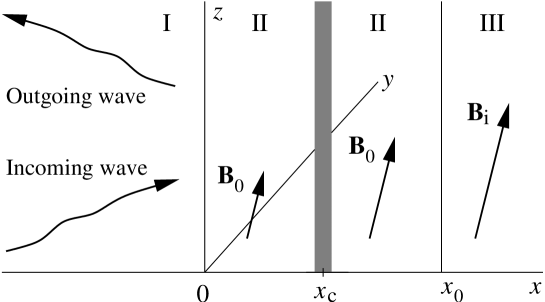
Figure 3: The sketch of the equilibrium state. The semi-infinite regions I ($x<0$) and III ($x>x_{0}$) contain homogeneous plasmas penetrated by homogeneous magnetic field, while the plasma and magnetic field in region II ($0<x<x_{0}$) are inhomogeneous. The resonant surface at $x=x_{c}$ is inside the dissipative layer shown by the shaded strip (adapted from Ruderman et al. 1997b and Ballai et al. 1998b).

All equilibrium quantities in region II depend on $x$ only. The equilibrium quantities are assumed to be continuous and satisfying the condition of the total pressure balance,

$$p_{e}=p_{0}(x)+\frac{B_{0}^{2}(x)}{2\mu_{0}}=p_{i}+\frac{B_{i}^{2}}{2\mu_{0}}.$$ (64)

This equation, in particular, implies that the ratio of equilibrium densities in regions III and I is given by

$$\frac{\rho_{i}}{\rho_{e}}=\frac{2c_{Se}^{2}}{2c_{Si}^{2}+\gamma v_{Ai}^{2}}.$$ (65)

The plasma dynamics outside the dissipative layer is described the system of linear ideal MHD equations. In what follows we consider solutions in the form of propagating waves with permanent shape, and assume that perturbations of all quantities depend on $x$ and $\theta=z-Vt$. Then the system of linear ideal MHD equations can be reduces to the system of two equations for the total pressure and $x$-component of the velocity,

$$\frac{\partial u}{\partial x}=\frac{V}{F}\frac{\partial P}{\partial\theta},\qquad\frac{\partial P}{\partial x}=\frac{\rho_{0}D_{A}}{V}\frac{\partial u}{\partial\theta},$$ (66)

where the quantities $F$ and $D_{A}$ are given by Eqs. (30) and (31). This system is written for region II. To use it in regions I and III we have to substitute $\rho_{0}$ by $\rho_{e}$ and $\rho_{i}$ respectively.

The physical picture of the wave interaction with the inhomogeneous plasma is as follows. The sound wave incoming from region I interacts with the inhomogeneous plasma in region II. It is partially reflected back in region I, partially penetrate in region III, and also partially absorbed in the dissipative layer. As a result we have an outgoing (or reflected) wave in region I in addition to the incoming wave and a transmitted wave in region III.

In what follows we assume that the incoming sound wave is monochromatic. We write its wave vector as $\vec{k}=(\chi k,0,k)$. Then its frequency is given by

$$\omega^{2}=k^{2}c_{Se}^{2}(1+\chi^{2}).$$ (67)

The solution to Eq. (66) describing the incoming wave can be written as

$$P=\epsilon p_{e}\cos[k(\theta+\chi x)],\quad u=\epsilon\frac{p_{e}\chi}{\rho_{e}V}\cos[k(\theta+\chi x)],$$ (68)

where $V=\omega/k=c_{Se}(1+\chi^{2})^{1/2}$. In general, the outgoing wave will contain not only the fundamental harmonic, but also the overtones. Hence, the expression for the pressure perturbation in the outgoing wave can be written as $P=\epsilon p_{e}A(\theta-\chi x)$, where $A$ is the function to be determined. Then the general solution to Eq. (66) describing the wave motion in region I is

$$P=\epsilon p_{e}\{\cos[k(\theta+\chi x)]+A(\theta-\chi x)\},\quad u=\epsilon\frac{p_{e}\chi}{\rho_{e}V}\{\cos[k(\theta+\chi x)]-A(\theta-\chi x)\}.$$ (69)

In region III the system of Eq. (66) can be reduced to

$$\frac{\partial P}{\partial x}+\kappa_{i}^{2}\frac{\partial P}{\partial\theta}=0,\quad\kappa_{i}^{2}=-\frac{V^{4}-V^{2}(c_{Si}^{2}+v_{Ai}^{2})+v_{Ai}^{2}c_{Si}^{2}\cos^{2}\alpha}{(c_{Si}^{2}+v_{Ai}^{2})(V^{2}-c_{Ti}^{2}\cos^{2}\alpha)}.$$ (70)

In what follows we assume that there is a resonance position $x_{c}$ in region II, so that $V=c_{T}(x_{c})\cos\alpha$. In addition we consider that $c_{T}(x)$ is a monotonically increasing function in region II. Then it is straightforward to show that $\kappa_{i}^{2}>0$, so that the wave motion in region III is evanescent. Using this result and expanding $P$ in the Fourier series with respect to $\theta$ we can write the solution to Eq. (66) decaying as $x\to\infty$ in the form

$$P=\sum_{n=-\infty}^{\infty}P_{n}\exp[k(in\theta-\kappa_{i}|n|(x-x_{0})],$$ (71)

where, at present, $P_{n}$ are arbitrary constants. Substituting this result in Eq. (66) we obtain that the $x$-component of the velocity in region III is given by

$$u=\frac{iV\kappa_{i}}{\rho_{i}(V^{2}-v_{Ai}^{2}\cos^{2}\alpha)}\sum_{n=-\infty}^{\infty}P_{n}\,{\rm sign}(n)\exp[k(in\theta-\kappa_{i}|n|(x-x_{0}))].$$ (72)

To obtain the solution in region II we expand $P$ and $u$ in the Fourier series with respect to $\theta$, and write the Fourier coefficients of these expansions as

$$P_{n}(x)=\rho_{e}V^{2}X_{n}(x),\quad u_{n}(x)=iVY_{n}(x).$$ (73)

Substituting these expressions in Eq. (66) we obtain the system of ordinary differential equations for $X_{n}$ and $Y_{n}$,

$$\frac{dX_{n}}{dx}=-\frac{\rho_{0}(V^{2}-v_{A}^{2}\cos^{2}\alpha)}{\rho_{e}V^{2}}nkY_{n},\quad\frac{dY_{n}}{dx}=\frac{\rho_{e}V^{2}}{F}nkX_{n}.$$ (74)

Consider the two solutions to this set of equations satisfying the boundary conditions at $x=0$,

$$X_{1n}^{-}=1,\quad Y_{1n}^{-}=0,$$ (75a)

$$X_{2n}^{-}=0,\quad Y_{2n}^{-}={\rm sign}(n),$$ (75b)

and the two solutions satisfying the boundary conditions at $x=x_{0}$,

$$X_{1n}^{+}=1,\quad Y_{1n}^{+}=0,$$ (76a)

$$X_{2n}^{+}=0,\quad Y_{2n}^{+}={\rm sign}(n).$$ (76b)

The solutions satisfying boundary conditions (75) are the two linearly independent solutions to the set of equations (74) regular in the interval $[0,x_{c})$. Any other solution regular in this interval can be written as a liner combination of these two solutions. Similarly, the solutions satisfying boundary conditions (76) are the two linearly independent solutions regular in the interval $(x_{c},x_{0}]$. Any other solution regular in this interval can be written as a liner combination of these two solutions.

Since the total pressure and $x$-component of the velocity are continuous at $x=0$ and $x=x_{0}$, the quantities $X_{n}$ and $Y_{n}$ satisfy the boundary conditions at $x=0$,

$$X_{n}=\frac{\epsilon p_{e}}{\rho_{e}V^{2}}\left(\frac{{}_{1}}{{}^{2}}\delta_{1|n|}+A_{n}\right),\quad Y_{n}=-\frac{i\epsilon\chi p_{e}}{\rho_{e}V^{2}}\left(\frac{{}_{1}}{{}^{2}}\delta_{1|n|}-A_{n}\right),$$ (77)

and at $x=x_{c}$,

$$X_{n}=\frac{P_{n}(x_{0})}{\rho_{e}V^{2}},\quad Y_{n}=\frac{\kappa\,{\rm sign}(n)P_{n}(x_{0})}{\rho_{i}(V^{2}-v_{Ai}^{2})},$$ (78)

where $\delta_{ij}$ is the Kronecker delta-symbol, and $A_{n}$ and $P_{n}$ are the coefficients in the expansions of functions $A(\theta)$ and $P(x,\theta)$ in the Fourier series with respect to $\theta$. Using these boundary conditions we immediately obtain that

$$X_{n}=\frac{\epsilon p_{e}}{\rho_{e}V^{2}}\left[\left(\frac{{}_{1}}{{}^{2}}\delta_{1|n|}+A_{n}\right)X_{1n}^{-}-i\chi\,{\rm sign}(n)\left(\frac{{}_{1}}{{}^{2}}\delta_{1|n|}-A_{n}\right)X_{2n}^{-}\right],$$ (79a)

$$Y_{n}=\frac{\epsilon p_{e}}{\rho_{e}V^{2}}\left[\left(\frac{{}_{1}}{{}^{2}}\delta_{1|n|}+A_{n}\right)Y_{1n}^{-}-i\chi\,{\rm sign}(n)\left(\frac{{}_{1}}{{}^{2}}\delta_{1|n|}-A_{n}\right)Y_{2n}^{-}\right],$$ (79b)

in $x<x_{c}$, and

$$X_{n}=\frac{P_{n}(x_{0})}{\rho_{e}V^{2}}\left(X_{1n}^{+}-\varsigma X_{2n}^{+}\right),\quad Y_{n}=\frac{P_{n}(x_{0})}{\rho_{e}V^{2}}\left(Y_{1n}^{+}-\varsigma Y_{2n}^{+}\right),$$ (80)

in $x>x_{c}$, where

$$\varsigma=\frac{\kappa\rho_{e}V^{2}}{\rho_{i}(v_{Ai}^{2}\cos^{2}\alpha-V^{2})}.$$ (81)

It follows from the first connection formula, Eq. (40), that $X_{n}(x)$ is continuous at $x=x_{c}$.

Equations (79) and (80) give the solution in region II. This solution contains the Fourier coefficients of the unknown function $A(\theta)$. Now we are in a position to derive the equation for $A(\theta)$. For this we calculate the jump of $u$ across the dissipative layer using Eqs. (79) and (80), and then compare it with the jump of $u$ given by the second connection formula. As a result we obtain the integral equation for $A(\theta)$.

Now we need to make one final remark. The procedure of derivation of the integral equation for $A(\theta)$ described above is only valid when the equilibrium magnetic field is in the $z$-direction, i.e. when $\alpha=0$. The reason is the following. We have assumed that $c_{T}(x)$ is a monotonically increasing function and the slow resonant position is determined by the equation $c_{T}(x_{c})\cos\alpha=V$. Since $v_{A}>c_{T}$, we have that $v_{A}(x_{c})\cos\alpha>V$. Since $v_{A}(0)=0$, this implies that there is at leas one point $x_{A}\in(0,x_{c})$ where $v_{A}(x_{A})\cos\alpha=V$, i.e. there is at least one Alfvén resonant position in $(0,x_{c})$. There is exactly one Alfvén resonant position when $v_{A}(x)$ is a monotonic function, while there could be a few Alfvén resonant positions if $v_{A}(x)$ is non-monotonic. In the simplest case when there is exactly one resonant position, $x_{A}<x_{c}$, we have to solve the ideal linear MHD equations in three intervals, $(0,x_{A})$, $(x_{A},x_{c})$ and $(x_{c},x_{0})$, use the solution to calculate the jumps of $u$ at $x_{A}$ and $x_{c}$, and then compare these jumps with those given by the connection formulae at the slow and Alfvén resonance. The case where $\alpha=0$ is exceptional because in this case there is no Alfvén resonance in spite that there is $x_{A}$ satisfying $v_{A}(x_{A})=V$.

7.1 Approximation of weak nonlinearity in dissipative layer

Ruderman et al. (1997b) studied the interaction of sound wave with an inhomogeneous plasma where the dominant dissipative processes are resistivity and isotropic viscosity under the assumption that $\alpha=0$. In the nonlinear theory, in general, we cannot obtain an explicit expression for $[u]$. To make analytical progress, however, Ruderman et al. (1997b) assumed that nonlinearity in the slow dissipative layer is weak and considered the nonlinear term in Eq. (37) as a perturbation. Then they carried out the asymptotic analysis using the modified nonlinearity parameter $N$ given by Eq. (48) as a small parameter. In particular, they calculated the coefficient of resonant absorption defined as

$$K=\frac{\Pi_{\rm in}-\Pi_{\rm out}}{\Pi_{\rm in}},$$ (82)

where $\Pi_{\rm in}$ and $\Pi_{\rm out}$ are the energy fluxes of the incoming and outgoing sound waves, respectively. They found that

$$K\approx K_{\rm L}+N^{2}K_{\rm cor},$$ (83)

where $K_{\rm L}$ is the coefficient of resonant absorption given by the linear theory, and $N^{2}K_{\rm cor}$ is the nonlinear correction, and obtained the analytical expressions for $K_{\rm L}$ and $K_{\rm cor}$ in the approximation of thin inhomogeneous layer ($kx_{0}\ll 1$). We do not give these expressions here. They can be found in Ruderman et al. (1997b). We only mention that $K_{\rm cor}<0$, so that nonlinearity supressess resonant absorption in the thin inhomogeneous layer approximation.

Ballai et al. (1998b) carried out a similar analysis but for plasmas where the dominant dissipative processes are compressional viscosity and thermal conduction, once again assuming that $\alpha=0$. They used $(kx_{0})N_{a}$ as a small parameter, where $N_{a}$ is given by Eq. (27). Ballai et al. (1998b) obtained the expression for $K$ similar to Eq. (83), however with $(kx_{0})N_{a}$ substituted for $N$. Once again, $K_{\rm cor}<0$ when $kx_{0}\ll 1$, however the expression for $K_{\rm cor}$ in terms of equilibrium quantities is different from that obtained by Ruderman et al. (1997b). The results obtained by Ruderman et al. (1997b) and Ballai et al. (1998b) clearly show that, while $K_{\rm L}$ remains the same no matter what type of dissipation operates in the slow dissipative layer, the coefficient of resonant absorption given by the nonlinear theory does depend on the dissipation type.

In a more recent study Clack and Ballai (2009a) investigated the efficiency of resonant absorption when inside the dissipative layer the dispersion was of the same order of magnitude as nonlinearity and dissipation. Using the limit of weak nonlinearity these authors found that the effect of dispersion is to increases the absolute value of the nonlinear correction (see Eq. 83), i.e. to decreases the net coefficient of absorption. Despite the change in the nonlinear correction this term still remained small compared to its linear counterpart.

7.2 Approximation of strong nonlinearity in dissipative layer

In this subsection we review studies about the same problem of absorption of the incoming wave energy in a slow resonant layer, however under assumption that the wave motion in the slow dissipative layer is strongly nonlinear. To simplify the analysis we assume that the equilibrium magnetic field is in the $z$-direction ($\alpha=0$), and region I is magnetic-free. The latter assumption implies that the incoming wave is a sound wave. The detailed investigation of this problem is given by Ruderman (2000). Here we only outline his analysis. In what follows we use the same notation as in Ruderman (2000).

The solution to the linear ideal MHD equations in regions I and III, and in region II outside the slow dissipative layer, have been already described above. As it has been explained, in order to obtain the equation for function $A(\theta)$ describing the outgoing wave we have to calculate $[u]$ using the solution of ideal linear MHD equations outside the dissipative layer, and then compare it with the expression for $[u]$ given by the second connection formula. In the case of strong nonlinearity in the dissipative layer this expression is given by Eq. (59). As a result we arrive at the integral equation determining $A(\theta)$,

$$M_{1}^{r}\cos(k\theta)+\chi M_{1}^{i}\sin(k\theta)+{\cal M}[A(\theta)]$$

$$\;\;=2k\zeta[S_{M}-S(\theta)]^{\frac{1}{2}}\left(\int_{\theta_{M}}^{\theta}[S_{M}-S(\tilde{\theta})]^{\frac{1}{2}}\,d\tilde{\theta}-\int_{\theta}^{L+\theta_{M}}[S_{M}-S(\tilde{\theta})]^{\frac{1}{2}}\,d\tilde{\theta}\right).$$ (84)

Here

$$S(\theta)=\frac{P_{c}(\theta)}{\epsilon p_{e}},\quad S_{M}=\frac{P_{M}}{\epsilon p_{e}},\quad\zeta=\frac{k\rho_{e}V^{6}}{\pi\rho_{0c}v_{Ac}^{4}|\Delta|}.$$ (85)

Recall that $P_{M}$ is the maximum value of $P$ in the dissipative layer. The operator ${\cal M}[A(\theta)]$ is given by

$${\cal M}[A(\theta)]=\sum_{n=1}^{\infty}\frac{1}{n}\left[M_{n}A_{n}\exp(ink\theta)+M_{n}^{*}A_{n}^{*}\exp(-ink\theta)\right],$$ (86)

where $A_{n}$ are the Fourier coefficients of function $A(\theta)$, the asterisk indicates the complex conjugate quantity, and the coefficients $M_{1}^{r}$, $M_{1}^{i}$ and $M_{n}$ are expressed in terms of the equilibrium quantities and the solutions $(X_{1n}^{\pm},Y_{1n}^{\pm})$ and $(X_{2n}^{\pm},Y_{2n}^{\pm})$ to the set of Eq. (74). We do not given these expressions here, they can be found in Ruderman (2000). The function $S(\theta)$ is expressed in terms of $A(\theta)$ by

$$S(\theta)=X_{11c}^{-}\cos(k\theta)+\chi X_{21c}^{-}\sin(k\theta)+{\cal L}[A(\theta)],$$ (87)

where the operator ${\cal L}[A(\theta)]$ is given by

$${\cal L}[A(\theta)]=\sum_{n=1}^{\infty}\left[(X_{1nc}^{-}+i\chi X_{2nc}^{-})A_{n}\exp(ink\theta)+(X_{1nc}^{-}-i\chi X_{2nc}^{-})A_{n}^{*}\exp(-ink\theta)\right].$$ (88)

Once again, the coefficients $X_{1nc}^{-}$ and $X_{2nc}^{-}$ are expressed in terms of the equilibrium quantities and the solutions to the set of Eq. (74). And, once again, we do not given these expressions here referring to Ruderman (2000) instead.

Since the operators ${\cal L}[A(\theta)]$ and ${\cal M}[A(\theta)]$ are expressed in terms of the Fourier coefficients of the function $A(\theta)$, and these Fourier coefficients, in turn, are expressed in terms of integrals of the function $A(\theta)$, the operators ${\cal L}[A(\theta)]$ and ${\cal M}[A(\theta)]$ are integral operators. Hence, Eq. (84) is the integral equation for the function $A(\theta)$.

In spite that Eq. (84) being a very complicated nonlinear equation, it has an extremely simple solution of the form

$$A(\theta)=a\cos(k\theta+\varphi),$$ (89)

where the quantities $a>0$ and $\varphi$ are expressed in terms of the equilibrium quantities and the solutions to the set of Eq. (74). We see that the outgoing wave is monochromatic in spite that the nonlinearity in the dissipative layer generates higher harmonics. The reason is that the amplitudes of these higher harmonics damp at distances of the order of thickness of the dissipative layer, so that only the fundamental harmonic survives at large distances from the slow resonant position.

Using the solution given by Eq. (89) Ruderman (2000) calculate the coefficient of resonant absorption. It immediately follows from Eq. (82) that $K=1-a^{2}$. Note that this expression is valid regardless whether we use the linear or nonlinear description of plasma motion in the slow dissipative layer. The nonlinearity only affects the value of $a$. In general, the set of Eq. (74) can be solved only numerically. However, in the thin inhomogeneous layer approximation $(kx_{0}\ll 1$) the analytical solution can be obtained in a straightforward way. In that case the expression for the coefficient of resonant absorption is given by

$$K_{\rm NL}=\frac{32\chi\zeta}{\chi^{2}+\varsigma^{2}}+{\cal O}(k^{2}x_{0}^{2}),$$ (90)

where we have used the subscript ‘NL’ to indicate that the coefficient of resonant absorption has been calculated using strongly nonlinear description of the wave motion in the slow dissipative layer. In Eq. (90) the quantity $\varsigma$ is given by Eq. (81) with $\alpha=0$, and $\zeta$ is given by Eq. (85). Note that $\zeta={\cal O}(kx_{0})$, so that $K_{\rm NL}={\cal O}(kx_{0})$, which implies that resonant absorption is weak in the thin inhomogeneous layer approximation. For the ratio of the coefficients of resonant absorption calculated using linear and strongly nonlinear descriptions we obtain

$$\frac{K_{\rm NL}}{K_{\rm L}}=\frac{8}{\pi^{2}}+{\cal O}(kx_{0})\approx 0.81.$$ (91)

We see that, in the thin inhomogeneous layer approximation, nonlinearity reduces the efficiency of resonant absorption. This result is in good agreement with the results obtained in the weak nonlinearity approximation and described in the previous subsection.

Ruderman (2000) studied numerically the dependence of $K_{\rm NL}/K_{\rm L}$ on $kx_{0}$ for different values of $\chi$ and a typical equilibrium. He found that $K_{\rm NL}/K_{\rm L}$ is a non-monotonic function of $kx_{0}$. First it grows, takes its maximum at $k_{m}x_{0}$, and then monotonically decreases. Typically $k_{m}x_{0}$ is between 4 and 6, and the maximum value of $K_{\rm NL}/K_{\rm L}$ is larger than 1. However the most important result is that, for $0<kx_{0}<10$, $K_{\rm NL}/K_{\rm L}$ does not deviate from unity by mode than 20%. Hence, we conclude that the effect of nonlinearity in slow dissipative layers on the coefficient of resonant absorption is moderate.

As pointed out previously, the nonlinear coefficient of resonant absorption depends on particular dissipative processes operating in a slow resonant layer. However, this dependence disappears in the approximation of strong nonlinearity. This result is related to the fact that, in the approximation of strong nonlinearity, dissipation in a slow resonant layer occurs not in the whole volume of this layer, but in slow shocks inside the layer. It is a very well known property of shocks that, while their internal structure is determined by particular dissipative processes operating in a shock, the amount of energy dissipated at the shock remains the same regardless what the dissipative processes are.

Recently Clack et al. (2010) introduced the concept of coupled resonances within the framework of nonlinear resonant MHD, where the transmitted waves at one of the resonances could play the role of the incoming wave for the second resonance. It is obvious that due to the $\beta\ll 1$ in the solar corona a coupled resonance (slow+Alfvén) would be impossible, however in plasmas where the plasma-$\beta$ is much closer to unity the coupled resonance could take place. In order to ensure that the second resonance takes place before the transmitted waves becomes evanescent, the proximity of the two resonances must be smaller than $k^{-1}$. When looking at the efficiency of the coupled resonances Clack et al. (2010) found that the absorption coefficient of the coupled resonance was larger than the sum of individual coefficients taken separately at the two resonances.

8 Generation of mean flows

When a wave propagates through a medium, the nonlinear interaction of the wave and medium generates a flow. This process is very well known in nonlinear acoustics where flows generated by propagating sound waves are called “acoustic flows” (see e.g. Rudenko and Soluyan, 1977).

We have already mentioned about the generation of flows by resonant MHD waves in Sect. 4 when we split the velocity in the slow dissipative layer in the mean and oscillatory parts. The flows very important for resonant and diagnostic purposes (see e.g. Doyle et al. (1997)). Ruderman et al. (1997a) derived the formulae determining the jumps of the derivative of the the mean flow across the dissipative layer under the assumptions that the plasma motion is periodic with the period $L$, and the dominant dissipative processes are isotropic viscosity and resistivity. Their study was later extended by Ballai et al. (2000b) for cylindrical geometries. These formulae determining the jumps can be written as

$$\left[\frac{d\bar{v}_{\perp}}{dx}\right]=\frac{\sin\alpha}{LV}\left(1+\frac{\rho_{0c}c_{Tc}^{2}\eta}{v_{Ac}^{2}\eta_{0}}\right)\int_{0}^{L}d\theta\int_{-\infty}^{\infty}\left(\frac{\partial\tilde{v}_{\parallel}}{\partial x}\right)^{2}dx,$$ (92)

$$\left[\frac{d\bar{v}_{\parallel}}{dx}\right]=-\frac{(\eta_{0}+\rho_{0c}\eta)V}{\eta_{0}v_{Ac}^{2}L\cos\alpha}\int_{0}^{L}d\theta\int_{-\infty}^{\infty}\left(\frac{\partial\tilde{v}_{\parallel}}{\partial x}\right)^{2}dx.$$ (93)

When the motion in a slow dissipative layer can be described by the linear dissipative MHD equations (which is possible if $N_{i}\ll 1$) we can find the explicit expression for the integrals in Eqs. (92) and (93) in terms of perturbation of total pressure $P$. In that case $\bar{v}_{\parallel}$ in the slow dissipative layer is described by Eq. (37) with the term proportional the time derivative and the nonlinear terms (which are the first and third term on the left-hand side) are neglected. This linear equation can be easily solved either by the method used by Goossens et al. (1995) or by the method used by Tirry and Goossens (1996) to obtain

$$\tilde{v}_{\parallel n}=-\frac{ic_{Tc}V^{2}P_{n}}{\rho_{0c}v_{Ac}^{2}\Delta_{c}}\left|\frac{2\pi n\Delta_{c}}{\lambda_{i}LV}\right|^{1/3}{\rm sign}(n\Delta_{c})F\bigg{(}(x-x_{c})\left|\frac{2\pi n\Delta_{c}}{\lambda_{i}LV}\right|^{1/3}{\rm sign}(n\Delta_{c})\bigg{)},$$ (94)

where $\tilde{v}_{\parallel n}$ and $P_{n}$ are the coefficients in the expansions of $\tilde{v}_{\parallel}$ and $P$ in the Fourier series with respect to $\theta$, and the $F$-function is defined by

$$F(y)=\int_{0}^{\infty}\exp(iy\sigma-\sigma^{3}/3)\,d\sigma.$$ (95)

Changing the order of integration and using the Parseval identity yields

$$\frac{1}{L}\int_{0}^{L}d\theta\int_{-\infty}^{\infty}\left(\frac{\partial\tilde{v}_{\parallel}}{\partial x}\right)^{2}dx=2\sum_{n=1}^{\infty}\int_{-\infty}^{\infty}\left|\frac{\partial\tilde{v}_{\parallel n}}{\partial x}\right|^{2}dx.$$ (96)

Using Eqs. (94) and (95) it is not difficult to obtain that

$$\int_{-\infty}^{\infty}\left|\frac{\partial\tilde{v}_{\parallel n}}{\partial x}\right|^{2}dx=\frac{2\pi^{2}c_{Tc}^{2}V^{3}n|P_{n}|^{2}}{\rho_{0c}^{2}v_{Ac}^{4}|\Delta_{c}|L\lambda_{i}}.$$ (97)

Substituting Eqs. (96) and (97) in Eqs. (92) and (93) we arrive at

$$\left[\frac{d\bar{v}_{\perp}}{dx}\right]=\frac{4\pi^{2}c_{Tc}^{2}V^{2}\sin\alpha}{\rho_{0c}v_{Ac}^{4}|\Delta_{c}|L\eta_{0}}\sum_{n=1}^{\infty}n|P_{n}|^{2},$$ (98)

$$\left[\frac{d\bar{v}_{\parallel}}{dx}\right]=-\frac{4\pi^{2}c_{Tc}^{4}V^{2}(\eta_{0}+\rho_{0c}\eta)\cos\alpha}{\rho_{0c}^{2}v_{Ac}^{6}|\Delta_{c}|L\eta_{0}}\left(\frac{\eta_{0}}{\rho_{0c}}+\frac{c_{Tc}^{2}\eta}{v_{Ac}^{2}}\right)^{-1}\sum_{n=1}^{\infty}n|P_{n}|^{2}.$$ (99)

It is instructive to estimate the order of magnitude of these jumps. It is not difficult to show that both jumps are of the order of $(V/L)N_{i}^{2}R_{e}\,R_{i}^{-4/3}$. It is interesting that, although the amplitude of the wave motion in the dissipative layers is small, the jumps given by Eqs. (98) and (99) can be quite large if $R_{e}\gg R_{m}$, i.e. if the magnetic Prandtl number, $P_{m}=\eta_{0}/\rho_{0c}\eta$, is small. Simple estimates show that these jumps are larger or of the order of $V/L$ when $1\ll R_{m}\ll R_{e}$ and $R_{e}\gtrsim\epsilon^{-2}$.

To find the profiles of the components of the mean velocity we need to impose boundary conditions far away from the dissipative layer. For example, if there are rigid walls at $x=\pm a$ where the condition of adhesion has to be satisfied, then the components of the mean velocity take the simple form

$$\bar{v}_{\perp}=\left\{\begin{array}[]{r}\displaystyle{\hskip 5.69054pt\left[\frac{d\bar{v}_{\perp}}{dx}\right]\frac{x-a}{2},\quad x<0,\vspace*{2mm}}\\ \displaystyle{-\left[\frac{d\bar{v}_{\perp}}{dx}\right]\frac{x+a}{2},\quad x>0,}\end{array}\right.\qquad\bar{v}_{\parallel}=\left\{\begin{array}[]{r}\displaystyle{\hskip 5.69054pt\left[\frac{d\bar{v}_{\parallel}}{dx}\right]\frac{x-a}{2},\quad x<0,\vspace*{2mm}}\\ \displaystyle{-\left[\frac{d\bar{v}_{\parallel}}{dx}\right]\frac{x+a}{2},\quad x>0.}\end{array}\right.$$ (100)

It is worth mentioning that the derivations carried in cylindrical geometry by Ballai et al. (2000b) resulted in some analogue relations for the jump in the mean flow components, but the properties of the mean flow generated by the nonlinear resonant slow waves are the same. This means that the results presented here are rather robust.

Although the dynamics of waves at the Alfvén resonance can be described within the framework of linear MHD with great accuracy, the process of resonance can produce a mean flow even in this later case. The problem of mean flow generation at the Alfvén resonance was recently studied by Clack and Ballai (2009b). In this case the jump in the oscillatory part of he parallel and perpendicular components of velocity are given as

$$\left[\frac{d\bar{v}_{\perp}}{dx}\right]=\frac{k^{2}\sin^{3}\alpha}{2\nu\rho_{0a}^{2}|\Delta_{a}|}\sum_{n=1}^{\infty}n|P_{n}|^{2},$$ (101)

and

$$\left[\frac{d\bar{v}_{\parallel}}{dx}\right]=-\frac{k^{2}\sin^{2}\alpha\cos\alpha}{2\nu\rho_{0a}^{2}|\Delta_{a}|}\sum_{n=1}^{\infty}n|P_{n}|^{2}.$$ (102)

For the particular case of $\alpha=\pi/4$ Clack and Ballai (2009b) found that these jumps scale as $\epsilon^{1/2}V/L$. For example, if the dimensionless amplitude $\epsilon={\cal O}(10^{-4})$ then the predicted mean shear flow is of the order of 10 km s^-1 in both upper chromosphere and solar corona. This value is comparable with observed values of bulk flow in coronal loops. However, we should keep in mind that the important difference between these two types of flows is their range; mean shear flows are rather localised while bulk motion of plasma occurs often along the entire coronal loop length.

Studies have been carried out to investigate the properties of shear flows, however nearly all of these have been numerical due to analytical complications when considering nonlinearity, turbulence and resonant absorption simultaneously. These studies have found that shear flows could give rise to a Kelvin-Helmholtz instability at the narrow dissipative layer (see, e.g. Terradas et al., 2008). This instability can drive turbulent motions and, in turn, locally enhance transport coefficients which can alter the efficiency of heating (see, e.g. Karpen et al., 1994; Ofman at al., 1994; Ofman and Davila, 1995). The generation of mean shear flow can supply additional shear enhancing turbulent motions.

9 Conclusions

Resonant absorption is a mechanism that ensures the effective transfer of energy between interacting systems. In solar and space plasmas resonant absorption is used in conjunction with the interaction of global waves and oscillations with inhomogeneous plasmas. Although the initial purpose of resonant absorption to be the phenomenon explaining the heating of solar corona seems these days a bit too optimistic, the advances of observational evidences of the last couple of years showed that resonant absorption is still a remarkable and brilliant mechanism on its own, able to explain a series of delicate effects occurring in the solar atmosphere and beyond.

The present review highlighted the progress made in the field of nonlinear resonance in the last 15 years. Simple estimations presented in this paper show that near resonances the amplitudes of oscillations can grow considerably and only a nonlinear description is adequate to describe accurately the physics near resonances. Luckily, as shown in the present review, these nonlinear additives to the effectiveness of absorption (compared to the linear counterpart) is not so significant, in general nonlinearity tends to decrease the net coefficient of absorption. In the case of resonant Alfvén waves, results show that the linear approach can give rather accurate results, with no need of using a mathematically more cumbersome nonlinear description.

We also showed that nonlinearity can have additional effects to the change in the absorption coefficient. Due to the nonlinear absorption of wave momentum in the vicinity of resonance, a shear mean flow is generated that is continuous across the layer containing the resonant surface, while its derivative has a jump. Simple estimations of the magnitude of the mean shear flow show that in the solar corona and upper chromosphere this mean flow is of the order of 10 km s^-1, a flow comparable with the existing bulk motion of the plasma in coronal loops. The generated shear flows can generate instabilities that can enhance locally the transport coefficients, i.e. the effectiveness of resonance.

The analysis on the nonlinear resonant absorption reviewed by our paper contains several simplifying assumptions that helped us progress in the analytical study of the process of nonlinear resonance. It is obvious that considerable advances in this field can be made only using numerical simulations. One way to extend the existing theories is the study of nonlinear absorption in 2-D geometries. Further, all presented theories supposed (and that is true for all studies of resonant absorption, including linear cases) that the interacting waves are monochromatic, however it is more likely that waves in nature do not depend on one single wavenumber, but they depend on a spectrum of values meaning that resonant absorption would occur for all those wavenumbers for which the resonant condition is satisfied (some encouraging numerical studies were carried earlier by Ofman and Davila 1996 and Ofman et al. 1998). It remains to be seen what subtle effects the mean shear flow has on the resonance, probably through numerical simulations. It also known through numerical investigations (see e.g. Ofman et al. 1998) that the resonant absorption leads to the modification of the loop density structure in the nonlinear regime, thus affecting the location, dynamics, and evolution of the resonant absorption layer, as well as the heating of the loop. This aspect still needs further investigation for the cases presented in our paper.

The abundance of high resolution observations and the extended numerical possibilities available will play an essential role in the progress of resonant absorption’s study and its applicability in explaining other phenomena occurring in solar and space plasmas predicting a bright future for this simple, yet fundamental effect in inhomogeneous space and laboratory plasmas.