Sulfate attack in sewer pipes: Derivation of a concrete corrosion model via two-scale convergence

Abstract

We explore the homogenization limit and rigorously derive upscaled equations for a microscopic reaction-diffusion system modeling sulfate corrosion in sewer pipes made of concrete. The system, defined in a periodically-perforated domain, is semi-linear, partially dissipative and weakly coupled via a non-linear ordinary differential equation posed on the solid-water interface at the pore level. Firstly, we show the well-posedness of the microscopic model. We then apply homogenization techniques based on two-scale convergence for an uniformly periodic domain and derive upscaled equations together with explicit formulae for the effective diffusion coefficients and reaction constants. We use a boundary unfolding method to pass to the homogenization limit in the non-linear ordinary differential equation. Finally, besides giving its strong formulation, we also prove that the upscaled two-scale model admits a unique solution.

and

1 Introduction

This paper treats the periodic homogenization of a semi-linear reaction-diffusion system coupled with a nonlinear differential equation arising in the modeling of the sulfuric acid attack in sewer pipes made of concrete. The concrete corrosion situation we are dealing with here strongly influences the durability of cement-based materials especially in hot environments leading to spalling of concrete and macroscopic fractures of sewer pipes. It is financially important to have a good estimate on the moment in time when such pipe systems need to be replaced, for instance, at the level of a city like Los Angeles. To get good such practical estimates, one needs on one side easy-to-use macroscopic corrosion models to be used for a numerical forecast of corrosion, while on the other side one needs to ensure the reliability of the averaged models by allowing them to incorporate a certain amount of microstructure information. The relevant question is: How much of this oscillatory-type information is needed to get a sufficiently accurate description of the heterogeneous reality? Due to the complexity of possible shapes of the microstructure, averaging concrete materials is far more difficult than averaging metallic composites with rigorously defined well-packed structure. In this paper, we imagine our concrete piece to be made of a periodically-distributed microstructure. Based on this assumption, we provide here a rigorous justification of the formal asymptotic expansion performed by us (in [1]) for this reaction-diffusion scenario. Note that in [1] upscaled models are derived for a more general situation involving a locally-periodic distribution of perforations. Locally periodic geometries refer to a special case of $x$-dependent microstructures, where, inherently, the outer normals to (microscopic) inner interfaces are dependent on both spatial slow variable, say $x$, and fast variable, say $y$.

In the framework of this paper, we combine two-scale convergence concepts with the periodic unfolding of interfaces to pass to the homogenization limit (i.e. to $\varepsilon\to 0$, where $\varepsilon$ is a small parameter linked to the relative size of the perforation) for the uniformly periodic case. Here, the outer normals to the inner interfaces are dependent only on the spatial fast variable. For more details on the mathematical modeling of sulfate corrosion of concrete, we refer the reader to [2, 3] (a moving-boundary approach: numerics and formal matched asymptotics), [4] (a two-scale reaction-diffusion system modeling sulfate corrosion), as well as to [5], where a nonlinear Henry-law type transmission condition (modeling $H_{2}S$ transfer across all air-water interfaces present in this sulfatation problem) is analyzed. Mathematical background on periodic homogenization can be found in e.g., [6, 7, 8], while a few relevant (remotely resembling) worked-out examples of this averaging methodology are explained, for instance, in [9, 10, 11, 12, 13, 14]. It is worth noting that, since it deals with the homogenization of a linear Henry-law setting, the paper [11] is related to our approach. The major novelty here compared to [11] is that we now need to pass to the limit in a non-dissipative object, namely a nonlinear ordinary differential equation (ode). The ode is describing sulfatation reaction at the inner water-solid interface – place where corrosion localizes. This aspect makes a rigorous averaging challenging. For instance, compactness-type methods do not work in the case when the nonlinear ode is posed on $\epsilon$-dependent surfaces. We circumvent this issue by ”boundary unfolding” the ode. Thus we fix, as independent of $\epsilon$, the reaction interface similarly as in [15], and only then we pass to the limit. Alternatively, one could use varifolds (cf. e.g. [16]), since this seems to be the natural framework for the rigorous passage to the limit when both the surface measure and the oscillating sequences depend on $\epsilon$. However, we find the boundary unfolding technique easier to adapt to our scenario than the varifolds.

Note that here we approach the corrosion problem deterministically. However, we have reasons to expect that the uniform periodicity assumption can be relaxed by assuming instead a Birkhoff-type ergodicity of the microstructure shapes and positions, and hence, the natural averaging context seems to be the one offered by random fields; see ch. 1, sect. 6 in [17], ch. 8 and 9 in [18], or [19]. But, methodologically, how big is the overlap between homogenizing deterministically locally-periodic distributions of microstructures compared to working in the random fields context? We will treat these and related aspects elsewhere.

The paper is organized as follows: We start off in section 2 (and continue in section 3) with the analysis of the microscopic model. In section 4, we obtain the $\varepsilon$-independent estimates needed for the passage to the limit $\varepsilon\to 0$. Section 5 contains the main result of the paper: the set of the upscaled two-scal equations.

2 The microscopic model

In this section, we describe the geometry of our array of periodic microstructures and briefly indicate the most aggressive chemical reaction mechanism typically active in sewer pipes. Finally, we list the set of microscopic equations.

2.1 Basic geometry

Fig. 1 (i) shows a cross-section of a sewer pipe hosting corrosion. We assume that the geometry of the porous medium in question consists of a system of pores periodically distributed inside the three-dimensional cube $\Omega:=[a,b]^{3}$ with $a,b\in\mathbb{R}$ and $b>a$. The exterior boundary of $\Omega$ consists of two disjoint, sufficiently smooth parts: ${\Gamma^{N}}$ - the Neumann boundary and ${\Gamma^{D}}$ - the Dirichlet boundary. The reference pore, say $Y:=[0,1]^{3}$, has three pairwise disjoint connected domains $Y^{s}$, $Y^{w}$ and $Y^{a}$ with smooth boundaries $\Gamma^{sw}$ and $\Gamma^{wa}$, as shown in Fig. 1 (iii). Moreover, $Y:=\bar{Y}^{s}\cup\bar{Y}^{w}\cup\bar{Y}^{a}$.

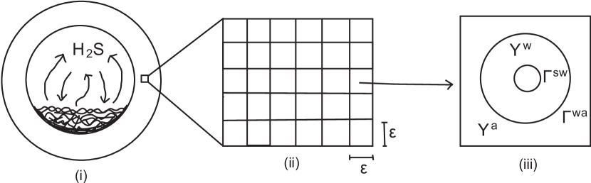
Figure 1: Left: Cross-section of a sewer pipe pointing out one region. Middle: Periodic approximation of the periodic rectangular domain. Right: Reference pore configuration.

Let $\varepsilon$ be a sufficiently small scaling factor denoting the ratio between the characteristic length of the pore $Y$ and the characteristic length of the domain $\Omega$. Let $\chi^{w}$ and $\chi^{a}$ be the characteristic functions of the sets $Y^{w}$ and $Y^{a}$, respectively. The shifted set $Y^{w}_{k}$ is defined by

$$Y^{w}_{k}:=Y+\Sigma_{j=0}^{3}k_{j}e_{j}\;\mbox{for}\;\;k=(k_{1},k_{2},k_{3})\in\mathbb{Z}^{3},$$

where $e_{j}$ is the $j^{th}$ unit vector. The union of all shifted subsets of $Y^{w}_{k}$ multiplied by $\varepsilon$ (and confined within $\Omega$) defines the perforated domain $\Omega^{\varepsilon}$, namely

$$\Omega^{\varepsilon}:=\cup_{k\in\mathbb{Z}^{3}}\{\varepsilon Y^{w}_{k}\;|\;\varepsilon Y^{w}_{k}\subset\Omega\}.$$

Similarly, $\Omega_{1}^{\varepsilon}$, $\Gamma^{sw}_{\varepsilon}$, and $\Gamma^{wa}_{\varepsilon}$ denote the union of the shifted subsets (of $\Omega$) $Y^{a}_{k}$, $\Gamma^{sw}_{k}$, and $\Gamma^{wa}_{k}$ scaled by $\varepsilon$. Since usually the concrete in sewer pipes is not completely dry, we decide to take into account a partially saturated porous material. We assume that every pore has three distinct non-overlapping parts: a solid part (grain) which is placed in the center of the pore, the water film which surrounds the solid part, and an air layer bounding the water film and filling the space of $Y$ as shown in Fig. 1. The air connects neighboring pores to one another. The geometry defined above satisfies the following assumptions:

1. Neither solid nor water-filled parts touch the boundary of the pore.

2. All internal (air-water and water-solid) interfaces are sufficiently smooth and do not touch each other.

These geometrical restrictions imply that the pores are connected by air-filled parts only which is needed not only to give a meaning to functions defined across interfaces, but also to introduce the concept of extension as given, for instance, in [20]. Furthermore, there are no solid-air interfaces.

2.2 Description of the chemistry

There are many variants of severe attack to concrete in sewer pipes, we focus here on the most aggressive one – the sulfuric acid attack. The situation can be described briefly as follows: (The anaerobic bacteria in the flowing waste water release hydrogen sulfide gas ($H_{2}S$) within the air space of the pipe. These bacteria are especially active in hot environments. From the air space inside the pipe, $H_{2}S(g)$ enters the pores of the concrete matrix where it diffuses and then dissolves in the pore water. The aerobic bacteria catalyze some of the $H_{2}S$ into sulfuric acid $H_{2}SO_{4}$. $H_{2}S$ molecules can move between air-filled part and water-filled part the water-air interfaces [21]. We model this microscopic interfacial transfer via Henry’s law [22], (see the boundary conditions at $\Gamma^{wa}_{\varepsilon}$ in (3) and (4)). $H_{2}SO_{4}$ being an aggressive acid reacts with the solid matrix at the solid-water interface, which is made up of cement, sand, and aggregate, and produces gypsum (i.e. $CaSO_{4}\cdot 2H_{2}O$). Here we restrict our attention to a minimal set of chemical reactions mechanisms as suggested in [2], namely.

$$\left\{\begin{aligned} 10H^{+}+SO_{4}^{-2}+\mbox{org. matter}\;&\longrightarrow\;H_{2}S(aq)+4H_{2}O+\mbox{oxid. matter}\\ H_{2}S(aq)+2O_{2}\;&{\longrightarrow}\;2H^{+}+SO_{4}^{-2}\\ H_{2}S(aq)\;&\rightleftharpoons\;H_{2}S(g)\\ 2H_{2}O+H^{+}+SO_{4}^{-2}+CaCO_{3}\;&{\longrightarrow}\;CaSO_{4}\cdot 2H_{2}O+HCO_{3}^{-}\end{aligned}\right.$$ (1)

We assume that reactions (1) do not interfere with the mechanics of the solid part of the pores. This is a rather strong assumption since it is known that (1) can actually produce local ruptures of the solid matrix [23]. For more details on the involved cement chemistry and connections to acid corrosion, we refer the reader to [24] (for a nice enumeration of the involved physicochemical mechanisms), [23] (standard textbook on cement chemistry), as well as to [25, 26, 27] and references cited therein. For a mathematical approach of a similar theme related to the conservation and restoration of historical monuments, we refer to the work by R. Natalini and co-workers (cf. e.g. [28]).

2.3 Setting of the equations

The data and unknown are given by

$${u^{\varepsilon}_{1}}_{0} :\Omega\longrightarrow\mathbb{R}_{+}\mbox{ - initial concentration of }H_{2}SO_{4}(aq)$$

$${u^{\varepsilon}_{2}}_{0} :\Omega\longrightarrow\mathbb{R}_{+}\mbox{ - initial concentration of }H_{2}S(aq)$$

$${u^{\varepsilon}_{3}}_{0} :\Omega\longrightarrow\mathbb{R}_{+}\mbox{ - initial concentration of }H_{2}S(g)$$

$${u^{\varepsilon}_{4}}_{0} :\Omega\longrightarrow\mathbb{R}_{+}\mbox{ - initial concentration of moisture}$$

$${u^{\varepsilon}_{5}}_{0} :\Omega\longrightarrow\mathbb{R}_{+}\mbox{ - initial concentration of gypsum}$$

$$u_{3}^{D} :\Gamma_{D}\times(0,T)\longrightarrow\mathbb{R}_{+}\mbox{ - exterior concentration (Dirichlet data) of }H_{2}S(g)$$

$$u^{\varepsilon}_{1} :\Omega^{\varepsilon}\times(0,T)\longrightarrow\mathbb{R}\mbox{ - concentration of }H_{2}SO_{4}(aq)$$

$$u^{\varepsilon}_{2} :\Omega^{\varepsilon}\times(0,T)\longrightarrow\mathbb{R}\mbox{ - concentration of }H_{2}S(aq)$$

$$u^{\varepsilon}_{3} :\Omega^{\varepsilon}_{1}\times(0,T)\longrightarrow\mathbb{R}\mbox{ - concentration of }H_{2}S(g)$$

$$u^{\varepsilon}_{4} :\Omega^{\varepsilon}\times(0,T)\longrightarrow\mathbb{R}\mbox{ - concentration of moisture}$$

$$u^{\varepsilon}_{5} :\Gamma^{sw}_{\varepsilon}\times(0,T)\longrightarrow\mathbb{R}\mbox{ - concentration of gypsum }$$

All concentrations are viewed as mass concentrations. We consider the following system of mass-balance equations defined at the pore level. The mass-balance equation for $H_{2}SO_{4}$ is

$$\partial_{t}u^{\varepsilon}_{1}+div(-d^{\varepsilon}_{1}\nabla u^{\varepsilon}_{1}) =-k^{\varepsilon}_{1}u^{\varepsilon}_{1}+k^{\varepsilon}_{2}u^{\varepsilon}_{2},\quad x\in\Omega^{\varepsilon},\;t\in(0,T)$$ (2)

$$u^{\varepsilon}_{1}(x,0) ={u^{\varepsilon}_{1}}_{0}(x),\quad x\in\Omega^{\varepsilon}$$

$$-n^{\varepsilon}\cdot d^{\varepsilon}_{1}\nabla u^{\varepsilon}_{1} =0,\quad x\in\Gamma^{wa}_{\varepsilon},\;t\in(0,T)$$

$$-n^{\varepsilon}\cdot d^{\varepsilon}_{1}\nabla u^{\varepsilon}_{1} =\varepsilon\eta(u^{\varepsilon}_{1},u^{\varepsilon}_{5}),\quad x\in\Gamma^{sw}_{\varepsilon}\;t\in(0,T).$$

The mass-balance equation for $H_{2}S(aq)$ is given by

$$\partial_{t}u^{\varepsilon}_{2}+div(-d^{\varepsilon}_{2}\nabla u^{\varepsilon}_{2}) =k^{\varepsilon}_{1}u^{\varepsilon}_{1}-k^{\varepsilon}_{2}u^{\varepsilon}_{2},\quad x\in\Omega^{\varepsilon},\;t\in(0,T),$$ (3)

$$u^{\varepsilon}_{2}(x,0) ={u^{\varepsilon}_{2}}_{0}(x),\quad x\in\Omega^{\varepsilon}$$

$$-n^{\varepsilon}\cdot d^{\varepsilon}_{2}\nabla u^{\varepsilon}_{2} =\varepsilon(a^{\varepsilon}(x)u^{\varepsilon}_{3}-b^{\varepsilon}(x)u^{\varepsilon}_{2}),\quad x\in\Gamma^{wa}_{\varepsilon},\;t\in(0,T)$$

$$-n^{\varepsilon}\cdot d^{\varepsilon}_{2}\nabla u^{\varepsilon}_{2} =0,\quad x\in\Gamma^{sw}_{\varepsilon},\;t\in(0,T).$$

The mass-balance equation for $H_{2}S(g)$ reads

$$\partial_{t}u^{\varepsilon}_{3}+div(-d^{\varepsilon}_{3}\nabla u^{\varepsilon}_{3}) =0,\quad x\in\Omega^{\varepsilon}_{1},\;t\in(0,T)$$ (4)

$$u^{\varepsilon}_{3}(x,0) ={u^{\varepsilon}_{3}}_{0}(x),\quad x\in\Omega^{\varepsilon}_{1}$$

$$-n^{\varepsilon}\cdot d^{\varepsilon}_{3}\nabla u^{\varepsilon}_{3} =0,\quad x\in\Gamma^{N},\;t\in(0,T)$$

$$u^{\varepsilon}_{3}(x,t) =u^{D}_{3}(x,t),\quad x\in\Gamma^{D},\;t\in(0,T)$$

$$-n^{\varepsilon}\cdot d^{\varepsilon}_{3}\nabla u^{\varepsilon}_{3} =-\varepsilon(a^{\varepsilon}(x)u^{\varepsilon}_{3}-b^{\varepsilon}(x)u^{\varepsilon}_{2}),\quad x\in\Gamma^{wa}_{\varepsilon},\;t\in(0,T).$$

The mass-balance equation for moisture follows

$$\partial_{t}u^{\varepsilon}_{4}+div(-d^{\varepsilon}_{4}\nabla u^{\varepsilon}_{4}) =k^{\varepsilon}_{1}u^{\varepsilon}_{1},\quad x\in\Omega^{\varepsilon},\;t\in(0,T)$$ (5)

$$u^{\varepsilon}_{4}(x,0) ={u^{\varepsilon}_{4}}_{0}(x),\quad x\in\Omega^{\varepsilon}$$

$$-n^{\varepsilon}\cdot d^{\varepsilon}_{4}\nabla u^{\varepsilon}_{4} =0,\quad x\in\Gamma^{wa}_{\varepsilon},\;t\in(0,T)$$

$$-n^{\varepsilon}\cdot d^{\varepsilon}_{4}\nabla u^{\varepsilon}_{4} =0,\quad x\in\Gamma^{sw}_{\varepsilon},\;t\in(0,T).$$

The mass-balance equation for the gypsum produced at the water-solid interface is

$$\partial_{t}u^{\varepsilon}_{5} =\eta(u^{\varepsilon}_{1},u^{\varepsilon}_{5}),\quad x\in\Gamma^{sw}_{\varepsilon},\;t\in(0,T)$$ (6)

$$u^{\varepsilon}_{5}(x,0) ={u^{\varepsilon}_{5}}_{0}(x),\quad x\in\Gamma^{sw}_{\varepsilon},\;t\in(0,T).$$

3 Weak formulation and basic results

We begin this section with a list of notations and function spaces. Then we indicate our working assumptions and give the weak formulation of the microscopic problem; we bring reader’s attention to the well-posedness of the system (2)–(6).

3.1 Notations and function spaces

We use $(\alpha,\beta)_{(0,T)\times\Omega^{\varepsilon}}:=\int_{0}^{T}\int_{\Omega^{\varepsilon}}\alpha\beta dxdt$, $(\alpha,\beta)_{(0,T)\times\Gamma_{\varepsilon}}:=\int_{0}^{T}\int_{\Gamma_{\varepsilon}}\alpha\beta d\sigma_{x}dt$. $\langle\cdot\rangle$, $|\cdot|$ and $\|\cdot\|$ denote the dual pairing of $H^{1}(\Omega^{\varepsilon})$ and $H^{-1}(\Omega^{\varepsilon})$, the norm in $L^{2}(\Omega^{\varepsilon})$, and the norm in $H^{1}(\Omega^{\varepsilon}),$ respectively. $\varphi^{+}$ and $\varphi^{-}$ will point out the positive and respectively the negative part of the function $\varphi$. We denote by $C^{\infty}_{\#}(Y)$, $H^{1}_{\#}(Y)$, and $H^{1}_{\#}(Y)/\mathbb{R}$, the space of infinitely differentiable functions in $\mathbb{R}^{n}$ that are periodic of period $Y$, the completion of $C^{\infty}_{\#}(Y)$ with respect to $H^{1}-$norm, and the respective quotient space, respectively. Furthermore, $H^{1}_{\Gamma^{D}}(\Omega):=\{u\in H^{1}(\Omega)|u=0\mbox{ on }\Gamma^{D}\}$. The Sobolev space $H^{\beta}(\Omega)$ as a completion of $C^{\infty}(\Omega)$ is a Hilbert space equipped with a norm

$$\|\varphi\|_{H^{\beta}(\Omega)}=\|\varphi\|_{H^{[\beta]}(\Omega)}+\left(\int_{\Omega}\int_{\Omega}\frac{|\varphi(x)-\varphi(y)|^{2}}{|x-y|^{n+2(\beta-[\beta])}}dxdy\right)^{\frac{1}{2}}$$

and (cf. Theorem 7.57 in [29]) the embedding $H^{\beta}(\Omega)\hookrightarrow L^{2}(\Omega)$ is continuous. Since we deal with an evolution problem, we need typical Bochner spaces like $L^{2}(0,T;H^{1}(\Omega))$, $L^{2}(0,T;H^{-1}(\Omega))$, $L^{2}(0,T;H^{1}_{\Gamma^{D}}(\Omega))$, and $L^{2}((0,T)\times\Omega;H^{1}_{\#}(Y)/\mathbb{R})$. In the analysis of the microscopic model, we use frequently the following trace inequality for $\varepsilon-$dependent hypersurfaces $\Gamma^{wa}_{\varepsilon}$: For $\varphi_{\varepsilon}\in H^{1}(\Omega^{\varepsilon})$, there exists a constant $C^{*}$, which is independent of $\varepsilon$, such that

$$\varepsilon|\varphi_{\varepsilon}|^{2}_{L^{2}(\Gamma_{\varepsilon})}\leq C^{*}(|\varphi_{\varepsilon}|^{2}_{L^{2}(\Omega^{\varepsilon})}+\varepsilon^{2}|\nabla\varphi_{\varepsilon}|^{2}_{L^{2}(\Omega^{\varepsilon})}).$$ (7)

The proof of (7) is given in Lemma 3 of [30]. For a function $\varphi^{\varepsilon}\in H^{\beta}(\Omega^{\varepsilon})$ with $\beta\in(\frac{1}{2},1)$, the inequality (7) refines into

$$\varepsilon|\varphi_{\varepsilon}|^{2}_{L^{2}(\Gamma_{\varepsilon})}\leq C^{*}_{0}(|\varphi_{\varepsilon}|^{2}_{L^{2}(\Omega^{\varepsilon})}+\varepsilon^{2\beta}\int_{\Omega}^{\varepsilon}\int_{\Omega}^{\varepsilon}\frac{|\varphi^{\varepsilon}(x)-\varphi^{\varepsilon}(y)|^{2}}{|x-y|^{n+2\beta}}dxdy),$$ (8)

where $C^{*}_{0}$ is again a constant independent of $\varepsilon$. For proof of (8), see [15]. To simplify the writing of some of the estimates, we employ the next set of notations:

$$d_{i} :=\min_{[0,T]\times\bar{\Omega}}\mid d_{i}^{\varepsilon}\mid,\;i\in\{1,2,3,4\},\quad\tilde{d}_{i}:=\min_{[0,T]\times\bar{\Omega}}\mid\tilde{d}_{i}^{\varepsilon}\mid,$$

$$D_{m} :=\max_{[0,T]\times\Omega^{\varepsilon}}|\partial_{t}d^{\varepsilon}_{m}|,\;m\in\{1,2,3\},\quad k_{j}:=\min_{[0,T]\times\bar{\Omega}}\mid k_{j}^{\varepsilon}\mid,\;j\in\{1,2\}$$

$$K_{j} :=\min_{[0,T]\times\bar{\Omega}}\mid\partial_{t}k_{j}^{\varepsilon}\mid,\quad\tilde{k}_{j}:=\min_{[0,T]\times\bar{\Omega}}\mid{\tilde{k}}_{j}^{\varepsilon}\mid,$$

$$k^{\infty}_{m} :=\sup_{(0,T)\times\Omega}\mid k_{m}^{\varepsilon}\mid,\quad\tilde{k}^{\infty}_{m}:=\sup_{(0,T)\times\Omega}\mid\tilde{k}_{m}^{\varepsilon}\mid,$$

$$K^{\infty}_{m} :=\sup_{(0,T)\times\Omega}\mid\partial_{t}k_{m}^{\varepsilon}\mid,\quad M_{i}:=\sup_{(0,T)\times\Omega}\mid u_{i}^{\varepsilon}\mid,\;i\in\{1,2,3,4,5\},$$

$$A^{\infty} :=\sup_{(0,T)\times\Gamma^{wa}_{\varepsilon}}|a_{\varepsilon}|,\;B^{\infty}:=\sup_{(0,T)\times\Gamma^{wa}_{\varepsilon}}|b_{\varepsilon}|,$$

$$A^{\infty} :=\sup_{(0,T)\times\Gamma^{wa}_{\varepsilon}}|\partial_{t}a_{\varepsilon}|,\;B^{\infty}:=\sup_{(0,T)\times\Gamma^{wa}_{\varepsilon}}|\partial_{t}b_{\varepsilon}|,$$

$$\tilde{a}^{\infty} :=\sup_{(0,T)\times\Gamma^{wa}}|\tilde{a}|,\;\tilde{b}^{\infty}:=\sup_{(0,T)\times\Gamma^{wa}}|\tilde{b}|,$$

$$Q^{\infty} :=\sup_{s\in(0,T)\times\Gamma^{sw}_{\varepsilon}}|Q(s)|,\quad\bar{\eta}:=||\eta||_{\infty},\quad\hat{\eta}:=||\partial_{t}\eta||_{\infty}.$$

3.2 Assumptions on the data and parameters

We consider the following restriction on the data and parameters:

1. $d_{i}\in L^{\infty}((0,T)\times Y)^{3\times 3}$, $\partial_{t}d_{i}\in L^{\infty}((0,T)\times Y)^{3\times 3}$, $\partial_{tt}d_{i}\in L^{\infty}((0,T)\times Y)^{3\times 3}$, $(d_{i}(t,x)\xi,\xi)\geq d_{i0}\mid\xi\mid^{2}$ for $d_{i0}>0$, for every $\xi\in\mathbb{R}^{3}$, $(t,x)\in(0,T)\times Y$, $i\in\{1,2,3,4\}$.

2. $\eta$ is measurable w.r.t. $t$ and $x$ and $\eta(\alpha,\beta)=k_{3}^{\varepsilon}R(\alpha)Q(\beta)$, $R$ is sub-linear and locally Lipschitz function and $Q$ is bounded and locally Lipschitz function such that

   $$R(\alpha)=\left\{\begin{array}[]{ccc}\mbox{positive},\;\;\mbox{if}\;\;\alpha\geq 0,\\ 0,\;\;\;\mbox{otherwise}\end{array}\right.\quad\quad Q(\beta)=\left\{\begin{array}[]{ccc}\mbox{positive},\;\;\mbox{if}\;\;\beta<\beta_{max},\\ 0,\;\;\;\mbox{otherwise}\end{array}\right.$$

   Additionally to (A2), we sometimes assume (A2)’, that is

3. $\partial_{t}\eta\leq\hat{\eta}$.

4. $u^{\varepsilon}_{i0}\in L^{2}(\Omega^{\varepsilon})\cap L_{+}^{\infty}(\Omega^{\varepsilon}),\;i\in\{1,2,4\}$, $u^{\varepsilon}_{30}\in L^{2}(\Omega^{\varepsilon}_{1})\cap L_{+}^{\infty}(\Omega^{\varepsilon}_{1})$, $u^{\varepsilon}_{50}\in L^{2}(\Gamma^{sw}_{\varepsilon})\cap L_{+}^{\infty}(\Gamma^{sw}_{\varepsilon})$.

5. $a^{\infty}M_{3}=b^{\infty}M_{2}$, $k^{\infty}_{1}M_{1}=M_{4}$, $k_{1}M_{1}=k^{\infty}_{2}M_{2}$.

6. $a,b\in{C}^{1}([0,T];C^{0,\alpha}(\Gamma^{wa})),a,b\geq 0$ in $[0,T]\times\Gamma^{wa},\partial_{t}a,\partial_{t}b\in L^{\infty}((0,T)\times\Gamma^{wa})$.

7. $\partial_{t}u_{3}^{D}$, $\partial_{tt}u_{3}^{D}$ and $\nabla\partial_{t}u_{3}^{D}$ are bounded.

8. $k_{3}\in C^{1}([0,T];C^{0,\alpha}(\Gamma^{sw}))$ and $k_{j}\in C^{1}([0,T];C^{0,\alpha}(\bar{Y}))$ for any $j\in\{1,2\}$ and $\alpha\in]0,1]$.

The assumptions (A1)–(A3), (A5), and (A6) are of technical nature. The first equality in (A4) points out an infinitely fast (equilibrium) Henry law, while the last two equalities remotely resemble a detailed balance in two of the involved chemical reactions.

3.3 Weak formulation of the microscopic model

Definition 1.

Assume (A1) and (A3). We call the vector $u^{\varepsilon}=(u^{\varepsilon}_{1},u^{\varepsilon}_{2},u^{\varepsilon}_{3},u^{\varepsilon}_{4},u^{\varepsilon}_{5})$, a weak solution to (2)–(6) if $u^{\varepsilon}_{j}\in L^{2}(0,T;H^{1}(\Omega^{\varepsilon})),\partial_{t}u^{\varepsilon}_{j}\in L^{2}(0,T;H^{-1}(\Omega^{\varepsilon})),j\in\{1,2,4\}$, $u^{\varepsilon}_{3}\in u_{3}^{D}+L^{2}(0,T;H_{\Gamma^{D}}^{1}(\Omega_{1}^{\varepsilon})),\partial_{t}u^{\varepsilon}_{3}\in u_{3}^{D}+L^{2}(0,T;H^{-1}(\Omega_{1}^{\varepsilon})),u^{\varepsilon}_{5}\in L^{\infty}((0,T)\times\Gamma^{sw}_{\varepsilon}),\partial_{t}u^{\varepsilon}_{5}\in L^{\infty}((0,T)\times\Gamma^{sw}_{\varepsilon})$ such that the following identities hold

$$\langle\partial_{t}u^{\varepsilon}_{1},\varphi_{1}\rangle_{(0,T)\times\Omega^{\varepsilon}} +(d_{1}\nabla u^{\varepsilon}_{1}),\nabla\varphi_{1})_{(0,T)\times\Omega^{\varepsilon}}$$ (12)

$$=-(k_{1}u^{\varepsilon}_{1},\varphi_{1})_{(0,T)\times\Omega^{\varepsilon}}+(k_{2}u^{\varepsilon}_{2},\varphi_{1})_{(0,T)\times\Omega^{\varepsilon}}$$

$$-\varepsilon(\eta(u^{\varepsilon}_{1},u^{\varepsilon}_{4}),\varphi_{1})_{(0,T)\times\Gamma^{sw}_{\varepsilon}},$$

$$\langle\partial_{t}u^{\varepsilon}_{2},\varphi_{2}\rangle_{(0,T)\times\Omega^{\varepsilon}} +(d^{\varepsilon}_{2}\nabla u^{\varepsilon}_{2}),\nabla\varphi_{2})_{(0,T)\times\Omega^{\varepsilon}}$$ (13)

$$=(k^{\varepsilon}_{1}u^{\varepsilon}_{1},\varphi_{2})_{(0,T)\times\Omega^{\varepsilon}}-(k^{\varepsilon}_{2}u^{\varepsilon}_{2},\varphi_{2})_{(0,T)\times\Omega^{\varepsilon}}$$

$$+\varepsilon(a_{\varepsilon}u^{\varepsilon}_{3},\varphi_{2})_{(0,T)\times\Gamma^{wa}_{\varepsilon}}-\varepsilon(a_{\varepsilon}u^{\varepsilon}_{2},\varphi_{2})_{(0,T)\times\Gamma^{wa}_{\varepsilon}},$$

$$\langle\partial_{t}u^{\varepsilon}_{3},\varphi_{3}\rangle_{(0,T)\times\Omega_{1}^{\varepsilon}} =-(d^{\varepsilon}_{3}\nabla u^{\varepsilon}_{3}),\nabla\varphi_{3})_{(0,T)\times\Omega_{1}^{\varepsilon}}$$ (14)

$$-\varepsilon(a_{\varepsilon}u^{\varepsilon}_{3},\varphi_{3})_{(0,T)\times\Gamma^{wa}_{\varepsilon}}+\varepsilon(a_{\varepsilon}u^{\varepsilon}_{2},\varphi_{3})_{(0,T)\times\Gamma^{wa}_{\varepsilon}},$$

$$\langle\partial_{t}u^{\varepsilon}_{4},\varphi_{4}\rangle_{(0,T)\times\Omega^{\varepsilon}} =-(d^{\varepsilon}_{4}\nabla u^{\varepsilon}_{4}),\nabla\varphi_{4})_{(0,T)\times\Omega^{\varepsilon}}+(k^{\varepsilon}_{1}u^{\varepsilon}_{1},\varphi_{4})_{(0,T)\times\Omega^{\varepsilon}}$$ (15)

for all $\varphi_{j}\in L^{2}(0,T;H^{1}(\Omega^{\varepsilon})),j\in\{1,2,4\}$ and $\varphi_{3}\in L^{2}(0,T;H_{\Gamma^{D}}^{1}(\Omega_{1}^{\varepsilon}))$ together with the ode

$$\partial_{t}u^{\varepsilon}_{5} = \eta(u^{\varepsilon}_{1},u^{\varepsilon}_{5})\;\;\mbox{a.e. on}\;\;(0,T)\times{\Gamma^{ws}_{\varepsilon}}$$ (16)

and the initial conditions

$$u^{\varepsilon}_{i}(0,x) =u^{\varepsilon}_{i0}(x)\;\;x\in\Omega^{\varepsilon}\mbox{ for all }i\in\{1,2,4\},$$ (17)

$$u^{\varepsilon}_{3}(0,x) =u^{\varepsilon}_{30}(x)\;\;x\in\Omega_{1}^{\varepsilon},$$

$$u^{\varepsilon}_{5}(0,x) =u^{\varepsilon}_{50}(x)\;\;x\in\Gamma^{ws}_{\varepsilon}.$$

3.4 Basic results

Lemma 2.

(Positivity and $L^{\infty}$-estimates) Assume (A1)-(A6), and let $t\in[0,T]$ be arbitrarily chosen. Then the following estimates hold:

• $u^{\varepsilon}_{i}(t)\geq 0,\;\;i\in\{1,2,4\}$ a.e. in ${\Omega^{\varepsilon}}$, $u^{\varepsilon}_{3}(t)\geq 0$ a.e. ${\Omega^{\varepsilon}_{1}}$ and $u^{\varepsilon}_{5}(t)\geq 0$ a.e. on $\Gamma^{ws}_{\varepsilon}$.

• $u^{\varepsilon}_{i}(t)\leq M_{i}$, $i\in\{1,2\}$, $u^{\varepsilon}_{4}(t)\leq(t+1)M_{4}$ a.e. in ${\Omega^{\varepsilon}}$ , $u^{\varepsilon}_{3}(t)\leq M_{3}$ a.e. in ${\Omega^{\varepsilon}_{1}}$ and $u^{\varepsilon}_{5}(t)\leq M_{5}$ a.e. on $\Gamma^{ws}_{\varepsilon}$.

Proof (i). We test (12)-(15) with $\varphi=(-{u^{\varepsilon}_{1}}^{-},-{u^{\varepsilon}_{2}}^{-},-{u^{\varepsilon}_{3}}^{-},-{u^{\varepsilon}_{4}}^{-})$ element of the space $[L^{2}(0,T;H^{1}(\Omega^{\varepsilon}))]^{2}\times L^{2}(0,T;H^{1}_{\Gamma^{D}}(\Omega_{1}^{\varepsilon})\times L^{2}(0,T;H^{1}(\Omega^{\varepsilon})$. We obtain the following inequality

$$\frac{1}{2}\partial_{t}|{u^{\varepsilon}_{1}}^{-}|^{2}+d_{1}|\nabla{u^{\varepsilon}_{1}}^{-}|^{2} \leq-k_{1}|{u^{\varepsilon}_{1}}^{-}|^{2}+k^{\infty}_{2}({u^{\varepsilon}_{1}}^{-},{u^{\varepsilon}_{2}}^{-})$$ (18)

$$-\varepsilon(\eta(u^{\varepsilon}_{1},u^{\varepsilon}_{5}),-{u^{\varepsilon}_{1}}^{-})_{\Gamma^{sw}_{\varepsilon}}.$$

Note that the first term on the r.h.s of (18) is negative, while the third term is zero because of (A2). We then get

$$\partial_{t}|{u^{\varepsilon}_{1}}^{-}|^{2}+2d_{1}|\nabla{u^{\varepsilon}_{1}}^{-}|^{2}\leq k^{\infty}_{2}\left(|{u^{\varepsilon}_{1}}^{-}|^{2}+|{u^{\varepsilon}_{2}}^{-}|^{2}\right).$$ (19)

On the other hand, (13) leads to

$$\frac{1}{2}\partial_{t}|{u^{\varepsilon}_{2}}^{-}|^{2}+d_{2}|\nabla{u^{\varepsilon}_{2}}^{-}|^{2} \leq\frac{k^{\infty}_{1}}{2}\left(|{u^{\varepsilon}_{1}}^{-}|^{2}+|{u^{\varepsilon}_{2}}^{-}|^{2}\right)$$

$$+\varepsilon a^{\infty}({u^{\varepsilon}_{2}}^{-},{u^{\varepsilon}_{3}}^{-})_{\Gamma^{wa}_{\varepsilon}}+\varepsilon b^{\infty}|{u^{\varepsilon}_{2}}^{-}|^{2}_{\Gamma^{wa}_{\varepsilon}}.$$

By the trace inequality (7) (with $\varepsilon<1$), we get

$$\partial_{t}|{u^{\varepsilon}_{2}}^{-}|^{2} +2(d_{2}-C^{*}b^{\infty})|\nabla{u^{\varepsilon}_{2}}^{-}|^{2}\leq{k^{\infty}_{1}}\left(|{u^{\varepsilon}_{1}}^{-}|^{2}+|{u^{\varepsilon}_{2}}^{-}|^{2}\right)$$ (20)

$$+2C^{*}b^{\infty}|{u^{\varepsilon}_{2}}^{-}|^{2}+2\varepsilon a^{\infty}({u^{\varepsilon}_{2}}^{-},{u^{\varepsilon}_{3}}^{-})_{\Gamma^{wa}_{\varepsilon}}.$$

(14) leads to

$$\partial_{t}|{u^{\varepsilon}_{3}}^{-}|^{2}+2(d_{3}-C^{*}a^{\infty})|\nabla{u^{\varepsilon}_{3}}^{-}|^{2}\leq 2\varepsilon b^{\infty}({u^{\varepsilon}_{2}}^{-},{u^{\varepsilon}_{3}}^{-})_{\Gamma^{wa}_{\varepsilon}}+2C^{*}a^{\infty}|{u^{\varepsilon}_{3}}^{-}|^{2},$$ (21)

while from (15), we see that

$$\partial_{t}|{u^{\varepsilon}_{4}}^{-}|^{2}+2d_{4}|\nabla{u^{\varepsilon}_{5}}^{-}|^{2}\leq k^{\infty}_{1}\left(|{u^{\varepsilon}_{1}}^{-}|^{2}+|{u^{\varepsilon}_{5}}^{-}|^{2}\right).$$ (22)

Adding up inequalities (19)-(22) gives

$$\partial_{t}\sum_{i=1}^{4}|{u^{\varepsilon}_{i}}^{-}|^{2} +2d_{1}|\nabla{u^{\varepsilon}_{1}}^{-}|^{2}+2(d_{2}-C^{*}b^{\infty})|\nabla{u^{\varepsilon}_{2}}^{-}|^{2}$$ (23)

$$+2(d_{3}-C^{*}a^{\infty})|\nabla{u^{\varepsilon}_{3}}^{-}|^{2}+2d_{4}|\nabla{u^{\varepsilon}_{4}}^{-}|^{2}$$

$$\leq\left(2k^{\infty}_{1}+k^{\infty}_{2}+2C^{*}b^{\infty}+2C^{*}a^{\infty}\right)\sum_{{i=1}}^{4}|{u^{\varepsilon}_{i}}^{-}|^{2}$$

$$+2\varepsilon(a^{\infty}+b^{\infty})({u^{\varepsilon}_{2}}^{-},{u^{\varepsilon}_{3}}^{-})_{\Gamma^{wa}_{\varepsilon}},$$

and hence,

$$\partial_{t}\sum_{i=1}^{4}|{u^{\varepsilon}_{i}}^{-}|^{2} +2d_{1}|\nabla{u^{\varepsilon}_{1}}^{-}|^{2}+2(d_{2}-C^{*}b^{\infty})|\nabla{u^{\varepsilon}_{2}}^{-}|^{2}$$ (24)

$$+2(d_{3}-C^{*}a^{\infty})|\nabla{u^{\varepsilon}_{3}}^{-}|^{2}+2d_{4}|\nabla{u^{\varepsilon}_{5}}^{-}|^{2}$$

$$\leq\left(2k^{\infty}_{1}+k^{\infty}_{2}+C^{*}(a^{\infty}+b^{\infty})\right)\sum_{i=1}^{4}|{u^{\varepsilon}_{i}}^{-}|^{2}$$

$$+\varepsilon\left(a^{\infty}+b^{\infty})(\delta|{u^{\varepsilon}_{2}}^{-}|_{\Gamma^{wa}_{\varepsilon}}^{2}+\frac{1}{\delta}|{u^{\varepsilon}_{3}}^{-}|^{2}_{\Gamma^{wa}_{\varepsilon}}\right).$$

Applying the trace inequality (7) to estimate the last term on the right side of (24), we finally get

$$\partial_{t}\sum_{i=1}^{4}|{u^{\varepsilon}_{i}}^{-}|^{2} +2d_{1}|\nabla{u^{\varepsilon}_{1}}^{-}|^{2}+(2d_{2}-2C^{*}b^{\infty}-C^{*}\delta(a^{\infty}+b^{\infty}))|\nabla{u^{\varepsilon}_{2}}^{-}|^{2}$$

$$+(2d_{3}-2C^{*}a^{\infty}-\frac{C^{*}2}{\delta}(a^{\infty}+b^{\infty}))|\nabla{u^{\varepsilon}_{3}}^{-}|^{2}+2d_{4}|\nabla{u^{\varepsilon}_{4}}^{-}|^{2}$$

$$\leq C_{1}\sum_{i=1}^{4}|{u^{\varepsilon}_{i}}^{-}|^{2}.$$

Thus, we have

$$\partial_{t}\sum_{i=1}^{4}|{u^{\varepsilon}_{i}}^{-}|^{2} \leq C_{1}\sum_{i=1}^{4}|{u^{\varepsilon}_{i}}^{-}|^{2}.$$

where $C_{1}:=2k^{\infty}_{1}+k^{\infty}_{2}+C^{*}(a^{\infty}+b^{\infty})+C^{*}(\delta+\frac{1}{\delta})(a^{\infty}+b^{\infty})$ and $\delta$ is chosen conveniently. Gronwall’s inequality together with $[u^{\varepsilon}_{i}(0)]^{-}=0$ gives now the desired result. Note that (A2) ensures automatically the positivity of $u^{\varepsilon}_{5}$.

(ii). We consider the test function

$$(\varphi_{1},\varphi_{2},\varphi_{3},\varphi_{4})=((u^{\varepsilon}_{1}-M_{1})^{+},(u^{\varepsilon}_{2}-M_{2})^{+},(u^{\varepsilon}_{3}-M_{3})^{+},(u^{\varepsilon}_{4}-(t+1)M_{4})^{+}).$$

Obviously, $\varphi\in[L^{2}(0,T;H^{1}(\Omega^{\varepsilon}))]^{2}\times L^{2}(0,T;H^{1}_{\Gamma^{D}}(\Omega_{1}^{\varepsilon})\times L^{2}(0,T;H^{1}(\Omega^{\varepsilon})$ is allowed as test function. We obtain from (12) that

$$\frac{1}{2}\partial_{t}|(u^{\varepsilon}_{1}-M_{1})^{+}|^{2} +d_{1}|\nabla(u^{\varepsilon}_{1}-M_{1})^{+}|^{2}\leq-k_{1}|(u^{\varepsilon}_{1}-M_{1})^{+}|^{2}$$

$$-(k_{1}M_{1},(u^{\varepsilon}_{1}-M_{1})^{+})$$

$$+k^{\infty}_{2}((u^{\varepsilon}_{1}-M_{1})^{+},(u^{\varepsilon}_{2}-M_{2})^{+})$$

$$+(k^{\infty}_{2}M_{2},(u^{\varepsilon}_{1}-M_{1})^{+})$$

$$-\varepsilon(\eta(u^{\varepsilon}_{1},u^{\varepsilon}_{5}),(u^{\varepsilon}_{1}-M_{1})^{+})_{\Gamma^{sw}_{\varepsilon}}.$$

Relying on (A4), we get the estimate

$$\begin{array}[]{ccc}\partial_{t}|(u^{\varepsilon}_{1}-M_{1})^{+}|^{2}&\leq&k^{\infty}_{2}(|(u^{\varepsilon}_{1}-M_{1})^{+}|^{2}+|(u^{\varepsilon}_{2}-M_{2})^{+}|^{2}).\end{array}$$ (26)

(13) in combination with (A4) gives that

$$\partial_{t}|(u^{\varepsilon}_{2}-M_{2})^{+}|^{2} +2(d_{2}-C^{*}b^{\infty})|\nabla(u^{\varepsilon}_{2}-M_{2})^{+}|^{2}$$ (27)

$$\leq k^{\infty}_{1}(|(u^{\varepsilon}_{1}-M_{1})^{+}|^{2}+|(u^{\varepsilon}_{2}-M_{2})^{+}|^{2})$$

$$+2C^{*}b^{\infty}|(u^{\varepsilon}_{2}-M_{2})^{+}|^{2}$$

$$+2\varepsilon a^{\infty}((u^{\varepsilon}_{2}-M_{2})^{+},(u^{\varepsilon}_{3}-M_{3})^{+})_{\Gamma^{wa}_{\varepsilon}}.$$

By (14), we obtain

$$\partial_{t}|(u^{\varepsilon}_{3}-M_{3})^{+}|^{2} +2(d_{3}-C^{*}a^{\infty})|\nabla(u^{\varepsilon}_{3}-M_{3})^{+}|^{2}$$ (28)

$$\leq 2C^{*}a^{\infty}|\nabla(u^{\varepsilon}_{3}-M_{3})^{+}|^{2}$$

$$+2\varepsilon b^{\infty}((u^{\varepsilon}_{2}-M_{2})^{+},(u^{\varepsilon}_{3}-M_{3})^{+})_{\Gamma^{wa}_{\varepsilon}}.$$

Using again (A4), (15) yields

$$\begin{array}[]{ccc}\partial_{t}|(u^{\varepsilon}_{4}-(t+1)M_{4})^{+}|^{2}&\leq&k^{\infty}_{1}(|(u^{\varepsilon}_{1}-M_{1})^{+}|^{2}+|(u^{\varepsilon}_{4}-(t+1)M_{4})^{+}|^{2}).\end{array}$$ (30)

Adding up (26)–(30) side by side, we get

$$\sum_{j=1}^{3}\partial_{t}|(u^{\varepsilon}_{j}-M_{j})^{+}|^{2} +\partial_{t}|(u^{\varepsilon}_{4}-(t+1)M_{4})^{+}|^{2}+(2d_{2}-2C^{*}b^{\infty})|\nabla(u^{\varepsilon}_{2}-M_{2})^{+}|^{2}$$

$$+(2d_{3}-2C^{*}a^{\infty})|\nabla(u^{\varepsilon}_{3}-M_{3})^{+}|^{2}$$

$$\leq(2k^{\infty}_{2}+k^{\infty}_{1}+2C^{*}a^{\infty}+2C^{*}b^{\infty})(\sum_{j=1}^{3}|(u^{\varepsilon}_{j}-M_{j})^{+}|^{2}$$

$$+|(u^{\varepsilon}_{4}-(t+1)M_{4})^{+}|^{2})+\varepsilon(a^{\infty}+b^{\infty})(\delta|(u^{\varepsilon}_{2}-M_{2})^{+}|^{2}_{\Gamma^{wa}_{\varepsilon}}$$

$$+\frac{1}{\delta}|(u^{\varepsilon}_{3}-M_{3})^{+}|^{2}_{\Gamma^{wa}_{\varepsilon}}).$$

We use the trace inequality (7) (with $\varepsilon<1$) to deal with the boundary terms in (3.4). Then Gronwall’s inequality yields for all $t\in(0,T)$ the following estimate

$$u^{\varepsilon}_{j}(t) \leq M_{j},\;\;j\in\{1,2,5\}\;a.\;e.\;in\;\Omega^{\varepsilon}$$

$$u^{\varepsilon}_{3}(t) \leq M_{3},\;a.\;e.\;in\;\Omega_{1}^{\varepsilon}$$

$$u^{\varepsilon}_{4} \leq(t+1)M_{4}\;\mbox{a.e. in}\;\Omega^{\varepsilon}.$$

Furthermore, by (A2) $u^{\varepsilon}_{5}$ is bounded.

Proposition 3.

(Uniqueness) Assume (A1)–(A4). Then there exists at most one weak solution in the sense of Definition 1.

Proof. We assume that ${u}^{j,\varepsilon}=(u_{1}^{j,\varepsilon},u_{2}^{j,\varepsilon},u_{3}^{j,\varepsilon},u_{4}^{j,\varepsilon},u_{5}^{j,\varepsilon}),j\in\{1,2\}$ are two distinct weak solutions in the sense of Definition 1. We set $u_{i}^{\varepsilon}:=u_{i}^{1,\varepsilon}-u_{i}^{2,\varepsilon}$ for all $i\in\{1,2,3,4\}$. Firstly, we deal with (15). We obtain

$$\partial_{t}{u^{1,\varepsilon}_{5}}-\partial_{t}{u^{2,\varepsilon}_{5}}=\eta(u^{1,\varepsilon}_{1},u^{1,\varepsilon}_{5})-\eta(u^{2,\varepsilon}_{1},u^{2,\varepsilon}_{5}).$$ (31)

Integrating (31) along (0,T) and using (A2), we get

$$|u^{1,\varepsilon}_{5}-u^{2,\varepsilon}_{5}|\leq k_{3}^{\infty}c_{R}c_{Q}M_{1}\int_{0}^{t}|{u^{1,\varepsilon}_{5}}-{u^{2,\varepsilon}_{5}}|d\tau+k_{3}^{\infty}c_{R}Q^{\infty}\int_{0}^{t}|{u^{1,\varepsilon}_{1}}-{u^{2,\varepsilon}_{1}}|d\tau.$$

Gronwall’s inequality implies

$$|{u^{1,\varepsilon}_{5}}(t)-{u^{2,\varepsilon}_{5}(t)}|\leq C_{2}\int_{0}^{t}|{u^{1,\varepsilon}_{1}}-{u^{2,\varepsilon}_{1}}|d\tau\;\;\mbox{for a.e. }t\in(0,T),$$ (32)

where $C_{2}:=k_{3}^{\infty}c_{R}Q^{\infty}(1+C_{3}te^{C_{3}t})$ and $C_{3}:=k_{3}^{\infty}c_{R}c_{Q}M_{1}$. We calculate

$$\frac{1}{2}\partial_{t}|{u^{\varepsilon}_{1}}|^{2}+d_{1}|\nabla{u^{\varepsilon}_{1}}|^{2}\leq-k_{1}|{u^{\varepsilon}_{1}}|^{2}+k^{\infty}_{2}({u^{\varepsilon}_{1}},{u^{\varepsilon}_{2}})+\varepsilon(\eta_{1}-\eta_{2},{u^{\varepsilon}_{1}})_{\Gamma^{sw}_{\varepsilon}},$$ (33)

where we denote $\eta_{1}-\eta_{2}:=\eta(u^{1,\varepsilon}_{1},u^{1,\varepsilon}_{5})-\eta(u^{2,\varepsilon}_{1},u^{2,\varepsilon}_{5})$. We can write

$$\frac{1}{2}\partial_{t}|{u^{\varepsilon}_{1}}|^{2}+d_{1}|\nabla{u^{\varepsilon}_{1}}|^{2} \leq-k_{1}|{u^{\varepsilon}_{1}}|^{2}+\frac{k^{\infty}_{2}}{2}(|{u^{\varepsilon}_{1}}|^{2}+|{u^{\varepsilon}_{2}}|^{2})$$ (34)

$$+\varepsilon C_{3}({u^{1,\varepsilon}_{5}}-{u^{2,\varepsilon}_{5}},{u^{\varepsilon}_{1}})_{\Gamma^{sw}_{\varepsilon}}$$

$$+\varepsilon k_{3}^{\infty}c_{R}Q^{\infty}({u^{1,\varepsilon}_{1}}-{u^{2,\varepsilon}_{1}},{u^{\varepsilon}_{1}})_{\Gamma^{sw}_{\varepsilon}}.$$

Now, inserting (32) in (34) yields

$$\frac{1}{2}\partial_{t}|{u^{\varepsilon}_{1}}|^{2}+d_{1}|\nabla{u^{\varepsilon}_{1}}|^{2} \leq-k_{1}|{u^{\varepsilon}_{1}}|^{2}+\frac{k^{\infty}_{2}}{2}(|{u^{\varepsilon}_{1}}|^{2}+|{u^{\varepsilon}_{2}}|^{2})$$ (35)

$$+C_{4}\varepsilon|{u^{\varepsilon}_{1}}|^{2}_{\Gamma^{sw}_{\varepsilon}}+\frac{\varepsilon C_{3}^{2}}{2\delta}\int_{0}^{t}|{u^{\varepsilon}_{1}}|^{2}_{\Gamma^{sw}_{\varepsilon}}d\tau,$$

where $C_{4}:=k_{3}^{\infty}c_{R}Q^{\infty}+\frac{C_{3}}{2\delta}$. Using (7), we estimate the last two terms in (35) to obtain the inequality

$$\frac{1}{2}\partial_{t}|{u^{\varepsilon}_{1}}|^{2}+d_{1}|\nabla{u^{\varepsilon}_{1}}|^{2} \leq-k_{1}|{u^{\varepsilon}_{1}}|^{2}+\frac{k^{\infty}_{2}}{2}(|{u^{\varepsilon}_{1}}|^{2}+|{u^{\varepsilon}_{2}}|^{2})+C^{*}C_{4}(|{u^{\varepsilon}_{1}}|^{2}$$ (36)

$$+\varepsilon^{2}|\nabla{u^{\varepsilon}_{1}}|)+C^{*}\frac{C_{3}^{2}}{2\delta}\int_{0}^{t}(|{u^{\varepsilon}_{1}}|^{2}+\varepsilon^{2}|\nabla{u^{\varepsilon}_{1}}|^{2})d\tau.$$

Note that the constant $C^{*}$, arising from in (36), stems from (7). Rearranging now the terms, we have

$$\partial_{t}|{u^{\varepsilon}_{1}}|^{2} +(2d_{1}-2C^{*}C_{4}\varepsilon^{2})|\nabla{u^{\varepsilon}_{1}}|^{2}+2k_{1}|{u^{\varepsilon}_{1}}|^{2}\leq({k^{\infty}_{2}}+C^{*}C_{4})(|{u^{\varepsilon}_{1}}|^{2}$$ (37)

$$+|{u^{\varepsilon}_{2}}|^{2})+C^{*}\frac{C_{3}^{2}}{2\delta}\int_{0}^{t}(|{u^{\varepsilon}_{1}}|^{2}+\varepsilon^{2}|\nabla{u^{\varepsilon}_{1}}|^{2})d\tau.$$

Following the same line of arguments as before, we obtain from (13) that

$$\partial_{t}|{u^{\varepsilon}_{2}}|^{2}+2d_{2}|\nabla{u^{\varepsilon}_{2}}|^{2} \leq-2k_{2}|{u^{\varepsilon}_{2}}|^{2}+{k^{\infty}_{1}}(|{u^{\varepsilon}_{1}}|^{2}+{u^{\varepsilon}_{2}}|^{2})$$ (38)

$$+2\varepsilon a^{\infty}({u^{\varepsilon}_{3}},{u^{\varepsilon}_{2}})_{\Gamma^{wa}_{\varepsilon}}+2\varepsilon b^{\infty}|{u^{\varepsilon}_{2}}|^{2}_{\Gamma^{wa}_{\varepsilon}},$$

while from (14), we deduce

$$\partial_{t}|{u^{\varepsilon}_{3}}|^{2}+2d_{3}|\nabla{u^{\varepsilon}_{3}}|^{2} \leq 2\varepsilon b^{\infty}({u^{\varepsilon}_{2}},{u^{\varepsilon}_{3}})_{\Gamma^{wa}_{\varepsilon}}+2\varepsilon a^{\infty}|{u^{\varepsilon}_{3}}|^{2}_{\Gamma^{wa}_{\varepsilon}}.$$ (39)

Proceeding similarly, (15) yields

$$\partial_{t}|{u^{\varepsilon}_{4}}|^{2}+2d_{4}|\nabla{u^{\varepsilon}_{4}}|^{2} \leq{k^{\infty}_{2}}(|{u^{\varepsilon}_{1}}|^{2}+|{u^{\varepsilon}_{4}}|^{2}).$$ (40)

Putting together (37)–(40), we get

$$\partial_{t}\Sigma^{4}_{i=1}|{u^{\varepsilon}_{i}}|^{2} +(2d_{1}-C^{*}C_{4}\varepsilon^{2})|\nabla{u^{\varepsilon}_{1}}|^{2}+2d_{2}|\nabla{u^{\varepsilon}_{2}}|^{2}+2d_{3}|\nabla{u^{\varepsilon}_{3}}|^{2}$$ (41)

$$+2d_{4}|\nabla{u^{\varepsilon}_{4}}|^{2}+2k_{1}|{u^{\varepsilon}_{1}}|^{2}$$

$$\leq\left(2{k^{\infty}_{1}}+{k^{\infty}_{2}}+C^{*}C_{2}\right)\Sigma^{4}_{i=1}|{u^{\varepsilon}_{i}}|^{2}$$

$$+C^{*}\frac{C_{1}^{2}}{2\delta}\int_{0}^{t}(|{u^{\varepsilon}_{1}}|^{2}+\varepsilon^{2}|\nabla{u^{\varepsilon}_{1}}|^{2})d\tau$$

$$+2\varepsilon b|{u^{\varepsilon}_{2}}|^{2}_{\Gamma^{wa}_{\varepsilon}}+2\varepsilon a|{u^{\varepsilon}_{3}}|^{2}_{\Gamma^{wa}_{\varepsilon}}$$

$$+\varepsilon(a^{\infty}+b^{\infty})(\delta|{u^{\varepsilon}_{2}}|_{\Gamma^{wa}_{\varepsilon}}^{2}+\frac{1}{\delta}|{u^{\varepsilon}_{3}}|_{\Gamma^{wa}_{\varepsilon}}^{2}).$$

Applying the trace inequality (7) to the boundary terms in (41), we get

$$\partial_{t}\Sigma^{4}_{i=1}|{u^{\varepsilon}_{i}}|^{2} +(2d_{1}-2C^{*}C_{4}\varepsilon^{2})|\nabla{u^{\varepsilon}_{1}}|^{2}$$

$$+(2d_{2}-2C^{*}b^{\infty}\varepsilon^{2}-C^{*}\delta\varepsilon^{2}(a^{\infty}+b^{\infty}))|\nabla{u^{\varepsilon}_{2}}|^{2}$$

$$+(2d_{3}-2C^{*}a^{\infty}\varepsilon^{2}-\frac{C^{*}\varepsilon^{2}}{\delta}(a^{\infty}+b^{\infty}))|\nabla{u^{\varepsilon}_{3}}|^{2}$$

$$+2d_{4}|\nabla{u^{\varepsilon}_{4}}|^{2}+2k_{1}|{u^{\varepsilon}_{1}}|^{2}\leq C_{5}\Sigma^{4}_{i=1}|{u^{\varepsilon}_{i}}|^{2}$$

$$+C^{*}\frac{C_{1}^{2}}{2\delta}\int_{0}^{t}(|{u^{\varepsilon}_{1}}|^{2}+\varepsilon^{2}|\nabla{u^{\varepsilon}_{1}}|^{2})d\tau,$$ (42)

where $C_{5}:=2{k^{\infty}_{1}}+{k^{\infty}_{2}}+C^{*}C_{2}+2C^{*}(a^{\infty}+b^{\infty})+C^{*}(a^{\infty}+b^{\infty})(\delta+\frac{1}{\delta})$. Let us choose $\varepsilon$ and $\delta$ such that

$$\varepsilon \in\left]0,\frac{2d_{1}}{C_{1}C^{*}}\right[$$

$$\delta \in\left[\frac{C^{*}\varepsilon^{2}(a^{\infty}+b^{\infty})}{2d_{3}-C^{*}a^{\infty}\varepsilon^{2}},\frac{2d_{2}-C^{*}b^{\infty}\varepsilon^{2}}{C^{*}\varepsilon^{2}(a^{\infty}+b^{\infty})}\right].$$

With this choice of $(\varepsilon,\delta)$, (42) takes the form

$$\partial_{t}\Sigma^{4}_{i=1}|{u^{\varepsilon}_{i}}|^{2}+\bar{C}|\nabla{u^{\varepsilon}_{1}}|^{2}+\bar{C}|{u^{\varepsilon}_{1}}|^{2}\leq{C_{6}}{}(\Sigma^{4}_{i=1}|{u^{\varepsilon}_{i}}|^{2}+\int_{0}^{t}(|{u^{\varepsilon}_{1}}|^{2}+\varepsilon^{2}|\nabla{u^{\varepsilon}_{1}}|^{2})d\tau),$$

where $C_{6}:=2{k^{\infty}_{1}}+{k^{\infty}_{2}}+C^{*}C_{2}+C^{*}(a^{\infty}+b^{\infty})+C^{*}\frac{C_{1}^{2}}{2\delta}$ and $\bar{C}:=\min\{2d_{1}-2C^{*}C_{2}\varepsilon^{2},2k_{1}\}$. Taking in (42) the supremum along $t\in(0,T)$ and applying Gronwall’s inequality, we obtain the following estimate

$$\Sigma^{4}_{i=1}|{u^{\varepsilon}_{i}}|^{2}+\bar{C}\int_{0}^{T}|\nabla{u^{\varepsilon}_{1}}|^{2}dt+\bar{C}\int_{0}^{T}|{u^{\varepsilon}_{1}}|^{2}dt\leq 0.$$ (43)

Thus, the proof of Proposition 3 is completed.

Theorem 4.

(Global Existence) Assume $(A1)-(A3)$. Then there exists at least a global-in-time weak solution in the sense of Definition 1.

Proof. The proof is based on the Galerkin argument. Since the proof is rather standard, and here we wish to focus on the passage to the limit $\varepsilon\to 0$, we omit it.

4 A priori estimates for microscopic solutions

This section includes the $\varepsilon-$ independent estimates.

Lemma 5.

Assume (A1)-(A6). Then the weak solution of the microscopic model (12)-(17) satisfies the following a priori bounds:

$$\parallel u^{\varepsilon}_{j}\parallel_{L^{2}(0,T;H^{1}(\Omega^{\varepsilon}))}\leq C,\;j\in\{1,2,3,4\}$$ (44)

$$\parallel\nabla\partial_{t}u^{\varepsilon}_{2}\parallel_{L^{2}(0,T;L^{2}(\Omega^{\varepsilon}))}\leq C,$$ (45)

$$\parallel\partial_{t}u^{\varepsilon}_{j}\parallel_{L^{2}(0,T;L^{2}(\Omega^{\varepsilon}))}\leq C,$$ (46)

$$\parallel u^{\varepsilon}_{3}\parallel_{L^{2}(0,T;H^{1}(\Omega^{\varepsilon}_{1}))}\leq C,$$ (47)

$$\parallel\nabla\partial_{t}u^{\varepsilon}_{3}\parallel_{L^{2}(0,T;L^{2}(\Omega^{\varepsilon}_{1}))}\leq C,$$ (48)

$$\parallel\partial_{t}u^{\varepsilon}_{3}\parallel_{L^{2}(0,T;L^{2}(\Omega^{\varepsilon}_{1}))}\leq C,$$ (49)

$$\parallel u^{\varepsilon}_{5}\parallel_{L^{\infty}((0,T)\times\Gamma^{sw}_{\varepsilon})}\leq C,$$ (50)

$$\parallel\partial_{t}u^{\varepsilon}_{5}\parallel_{L^{2}((0,T)\times\Gamma^{sw}_{\varepsilon})}\leq C.$$ (51)

In (44)–(51), the generic constant $C$ is independent of $\varepsilon$.

Proof. We test (12) with $\varphi_{1}=u^{\varepsilon}_{1}$ to get

$$\frac{1}{2}\partial_{t}|u^{\varepsilon}_{1}|^{2}+d_{1}|\nabla u^{\varepsilon}_{1}|^{2} \leq-k_{1}|u^{\varepsilon}_{1}|^{2}+k_{2}^{\infty}(u^{\varepsilon}_{1},u^{\varepsilon}_{2})-\varepsilon(\eta,u^{\varepsilon}_{1})_{\Gamma^{sw}_{\varepsilon}},$$ (52)

$$\leq\frac{k_{2}^{\infty}}{2}(|u^{\varepsilon}_{1}|^{2}+|u^{\varepsilon}_{2}|^{2})+\varepsilon k^{\infty}_{3}Q^{\infty}c_{R}(u^{\varepsilon}_{1},u^{\varepsilon}_{1})_{\Gamma^{sw}_{\varepsilon}}.$$

After applying the trace inequality to the last term on r.h.s of (52), we get

$$\frac{1}{2}\partial_{t}|u^{\varepsilon}_{1}|^{2}+d_{1}|\nabla u^{\varepsilon}_{1}|^{2} \leq\frac{k_{2}^{\infty}}{2}(|u^{\varepsilon}_{1}|^{2}+|u^{\varepsilon}_{2}|^{2})+C^{*}k^{\infty}_{3}Q^{\infty}c_{R}(|u^{\varepsilon}_{1}|^{2}+\varepsilon^{2}|\nabla u^{\varepsilon}_{1}|^{2})_{\Gamma^{sw}_{\varepsilon}}.$$

$$\frac{1}{2}\partial_{t}|u^{\varepsilon}_{1}|^{2} +(d_{1}-\varepsilon^{2}C^{*}k^{\infty}_{3}Q^{\infty}c_{R})|\nabla u^{\varepsilon}_{1}|^{2}\leq C_{7}(|u^{\varepsilon}_{1}|^{2}+|u^{\varepsilon}_{2}|^{2}),$$ (53)

where $C_{7}:=\frac{k_{2}^{\infty}}{2}+C^{*}k^{\infty}_{3}Q^{\infty}c_{R}.$ Taking $\varphi_{2}=u^{\varepsilon}_{2}$ in (13), we get

$$\frac{1}{2}\partial_{t}|u^{\varepsilon}_{2}|^{2}+d_{2}|\nabla u^{\varepsilon}_{2}|^{2} \leq\frac{k_{1}^{\infty}}{2}(|u^{\varepsilon}_{1}|^{2}+|u^{\varepsilon}_{2}|^{2})-k_{2}|u^{\varepsilon}_{2}|^{2}$$

$$+\varepsilon a^{\infty}(u^{\varepsilon}_{3},u^{\varepsilon}_{2})_{\Gamma^{wa}_{\varepsilon}}+\varepsilon b^{\infty}|u^{\varepsilon}_{2}|^{2}_{\Gamma^{wa}_{\varepsilon}}.$$

Application of the trace inequality (7) only to the last term leads to

$$\frac{1}{2}\partial_{t}|u^{\varepsilon}_{2}|^{2}+(d_{2}-C^{*}b^{\infty}\varepsilon^{2})|\nabla u^{\varepsilon}_{2}|^{2} \leq\frac{k_{1}^{\infty}}{2}(|u^{\varepsilon}_{1}|^{2}+|u^{\varepsilon}_{2}|^{2})+2$$ (54)

$$+\varepsilon a^{\infty}(u^{\varepsilon}_{3},u^{\varepsilon}_{2})_{\Gamma^{wa}_{\varepsilon}}.$$

We choose $\varphi_{3}=u^{\varepsilon}_{3}$ as a test function in (14) to calculate

$$\frac{1}{2}\partial_{t}|u^{\varepsilon}_{3}|^{2}+(d_{3}-C^{*}a^{\infty}\varepsilon^{2})|\nabla u^{\varepsilon}_{3}|^{2} \leq\varepsilon b^{\infty}(u^{\varepsilon}_{3},u^{\varepsilon}_{2})_{\Gamma^{wa}_{\varepsilon}}+C^{*}a^{\infty}|u^{\varepsilon}_{3}|^{2}.$$ (55)

Setting $\varphi_{4}=u^{\varepsilon}_{4}$ in (15), we are led to

$$\frac{1}{2}\partial_{t}|u^{\varepsilon}_{4}|^{2}+d_{4}|\nabla u^{\varepsilon}_{4}|^{2} \leq \frac{k_{1}^{\infty}}{2}(|u^{\varepsilon}_{1}|^{2}+|u^{\varepsilon}_{4}|^{2}).$$ (56)

Putting together (53)-(56), we obtain

$$\frac{1}{2}\Sigma_{i=1}^{4}\partial_{t}|u^{\varepsilon}_{i}|^{2} +(d_{1}-\varepsilon^{2}C^{*}k^{\infty}_{3}Q^{\infty}c_{R})|\nabla u^{\varepsilon}_{1}|^{2}+d_{4}|\nabla u^{\varepsilon}_{4}|^{2}$$ (57)

$$+(d_{2}-C^{*}b^{\infty}\varepsilon^{2})|\nabla u^{\varepsilon}_{2}|^{2}+(d_{3}-C^{*}a^{\infty}\varepsilon^{2})|\nabla u^{\varepsilon}_{3}|^{2}$$

$$\leq({k_{1}^{\infty}}{}+\frac{k_{2}^{\infty}}{2}+C^{*}b^{\infty}+C^{*}a^{\infty})\Sigma_{i=1}^{4}|u^{\varepsilon}_{i}|^{2}$$

$$+\varepsilon(a^{\infty}+b^{\infty})(u^{\varepsilon}_{3},u^{\varepsilon}_{2})_{\Gamma^{wa}_{\varepsilon}}.$$

Combing Young’s inequality and the trace inequality to the boundary term, (57) turns out to be

$$\frac{1}{2}\Sigma_{i=1}^{4}\partial_{t}|u^{\varepsilon}_{i}|^{2} +(d_{1}-\varepsilon^{2}C^{*}k^{\infty}_{3}Q^{\infty}c_{R})|\nabla u^{\varepsilon}_{1}|^{2}$$

$$+(d_{2}-C^{*}b\varepsilon^{2}-\frac{C^{*}\varepsilon^{2}\delta}{2}(a^{\infty}+b^{\infty}))|\nabla u^{\varepsilon}_{2}|^{2}$$

$$+(d_{3}-C^{*}a\varepsilon^{2}-\frac{C^{*}\varepsilon^{2}}{2\delta}(a^{\infty}+b^{\infty}))|\nabla u^{\varepsilon}_{3}|^{2}+d_{4}|\nabla u^{\varepsilon}_{4}|^{2}$$

$$\leq({k_{1}^{\infty}}{}+\frac{k_{2}^{\infty}}{2}+C^{*}(a^{\infty}+b^{\infty})(\delta+\frac{1}{\delta}))\Sigma_{i=1}^{4}|u^{\varepsilon}_{i}|^{2}.$$

Choosing $\varepsilon$ small enough and $\delta$ conveniently such that the coefficients of the terms involving $|\nabla u^{\varepsilon}_{2}|^{2}$ and $|\nabla u^{\varepsilon}_{3}|^{2}$ stay positive, we are led to

$$\Sigma_{i=1}^{4}\partial_{t}|u^{\varepsilon}_{i}|^{2}+d^{\prime}_{1}|\nabla u^{\varepsilon}_{1}|^{2}+d^{\prime}_{2}|\nabla u^{\varepsilon}_{2}|^{2}+d^{\prime}_{3}|\nabla u^{\varepsilon}_{3}|^{2} + 2d_{4}|\nabla u^{\varepsilon}_{4}|^{2}\leq C_{7}\Sigma_{i=1}^{4}|u^{\varepsilon}_{i}|^{2},$$

where

$$d^{\prime}_{1} :=2(d_{1}-\varepsilon^{2}C^{*}k^{\infty}_{3}Q^{\infty}c_{R}),$$

$$d^{\prime}_{2} :=2(d_{2}-C^{*}b^{\infty}\varepsilon^{2}-\frac{C^{*}\varepsilon^{2}\delta}{2}(a^{\infty}+b^{\infty})),$$

$$d^{\prime}_{3} :=2(d_{3}-C^{*}a^{\infty}\varepsilon^{2}-\frac{C^{*}b\varepsilon^{2}}{2\delta}(a^{\infty}+b^{\infty})),$$

while the constant $C$ is given by

$$C_{8}:=2{k_{1}^{\infty}}{}+\frac{k_{2}^{\infty}}{2}+C^{*}a^{\infty}+C^{*}b^{\infty}+C^{*}(a^{\infty}+b^{\infty})(\delta+\frac{1}{\delta}).$$

Summarizing, we have

$$\Sigma_{i=1}^{4}\partial_{t}|u^{\varepsilon}_{i}|^{2}+d_{0}\Sigma_{j=1}^{3}|\nabla u^{\varepsilon}_{j}|^{2}+d_{0}|\nabla u^{\varepsilon}_{3}|^{2}\leq C\Sigma_{i=1}^{4}|u^{\varepsilon}_{i}|^{2},$$ (58)

where $d_{0}:=min\{d^{\prime}_{1},d^{\prime}_{2},d^{\prime}_{3},d^{\prime}_{4}\}$. By Gronwall’s inequality, we have

$$\Sigma_{i=1}^{4}|u^{\varepsilon}_{i}|^{2}\leq C\Sigma_{i=1}^{4}|u_{i}(0)|^{2},$$

and hence,

$$\parallel u^{\varepsilon}_{j}\parallel_{L^{2}(0,T;L^{2}(\Omega^{\varepsilon}))}\leq C\mbox{ for all }i\in\{1,2,4\}\;\mbox{and}\;\|u^{\varepsilon}_{3}\|_{{L^{2}(0,T;L^{2}(\Omega^{\varepsilon}_{1}))}}\leq C,$$ (59)

where $C$ depends on initial data and model parameters but is independent of $\varepsilon$. Integrating (58) along $(0,T)$, we get

$$\parallel u^{\varepsilon}_{j}\parallel_{L^{2}(0,T;H^{1}(\Omega^{\varepsilon}))} \leq C,\;j\in\{1,2,4\},$$ (60)

$$\parallel u^{\varepsilon}_{3}\parallel_{L^{2}(0,T;H^{1}(\Omega^{\varepsilon}_{1}))} \leq C.$$

With the help of (A2) together with the boundedness of $u^{\varepsilon}_{1}$, we conclude from (16) that

$$\parallel u^{\varepsilon}_{5}\parallel_{L^{\infty}((0,T)\times\Gamma^{sw}_{\varepsilon})}\leq C.$$

Multiplying (16) by $\partial_{t}u^{\varepsilon}_{5}$ and using (A2), we get

$$\|\partial_{t}u^{\varepsilon}_{5}\|_{L^{2}((0,T)\times\Gamma^{sw}_{\varepsilon})}\leq C.$$

Now, we focus on obtaining $\varepsilon-$independent estimates on the time derivative of the concentrations. Firstly, we choose $\varphi_{1}=\partial_{t}u^{\varepsilon}_{1}$ and get

$$\int_{0}^{t}\int_{\Omega^{\varepsilon}}\partial_{t}u^{\varepsilon}_{1}\partial_{t}u^{\varepsilon}_{1}dxd\tau +\int_{0}^{t}\int_{\Omega^{\varepsilon}}d_{1}^{\varepsilon}\nabla u^{\varepsilon}_{1}\nabla\partial_{t}u^{\varepsilon}_{1}dxd\tau$$ (61)

$$=-\int_{0}^{t}\int_{\Omega^{\varepsilon}}k^{\varepsilon}_{1}u^{\varepsilon}_{1}\partial_{t}u^{\varepsilon}_{1}dxd\tau+\int_{0}^{t}\int_{\Omega^{\varepsilon}}k^{\varepsilon}_{2}u^{\varepsilon}_{2}\partial_{t}u^{\varepsilon}_{1}dxd\tau$$

$$-\varepsilon\int_{0}^{t}\int_{\Gamma^{sw}_{\varepsilon}}\eta\partial_{t}u^{\varepsilon}_{1}d\sigma_{x}d\tau.$$

Consequently, it holds

$$\int_{0}^{t}\int_{\Omega^{\varepsilon}}|\partial_{t}u^{\varepsilon}_{1}|^{2}dxd\tau +\int_{0}^{t}\int_{\Omega^{\varepsilon}}\left(\frac{1}{2}\partial_{t}(d_{1}^{\varepsilon}|\nabla u^{\varepsilon}_{1}|^{2})-(\partial_{t}d_{1}^{\varepsilon})|\nabla u^{\varepsilon}_{1}|^{2}\right)dxd\tau$$

$$\leq-\frac{k_{1}}{2}\int_{0}^{t}\int_{\Omega^{\varepsilon}}\partial_{t}|u^{\varepsilon}_{1}|^{2}dxd\tau$$

$$+\frac{k_{2}^{\infty}}{2}\int_{0}^{t}\int_{\Omega^{\varepsilon}}\left(\frac{1}{\delta}|u^{\varepsilon}_{2}|^{2}+\delta|\partial_{t}u^{\varepsilon}_{1}|^{2}\right)dxd\tau$$

$$-{\varepsilon}{}\int_{0}^{t}\int_{\Gamma^{sw}_{\varepsilon}}(\partial_{t}(\eta u^{\varepsilon}_{1})-(\partial_{t}\eta)u^{\varepsilon}_{1})d\sigma_{x}d\tau,$$

$$(1-\frac{k_{2}^{\infty}\delta}{2})\int_{0}^{t}\int_{\Omega^{\varepsilon}}|\partial_{t}u^{\varepsilon}_{1}|^{2}dxd\tau \leq D_{1}\int_{0}^{t}\int_{\Omega^{\varepsilon}}|\nabla u^{\varepsilon}_{1}|^{2}dxd\tau$$ (62)

$$+\frac{d_{1}^{\infty}}{2}\int_{\Omega^{\varepsilon}}|\nabla{u_{1}}_{0}|^{2}dx+\frac{k_{2}^{\infty}}{2\delta}\int_{0}^{t}\int_{\Omega^{\varepsilon}}|u^{\varepsilon}_{2}|^{2}dxd\tau$$

$$+\frac{\varepsilon}{2}\int_{\Gamma^{sw}_{\varepsilon}}\left(|\eta|^{2}+|u^{\varepsilon}_{1}|^{2}+|\eta(0)|^{2}+|u^{\varepsilon}_{1}(0)|^{2}\right)d\sigma_{x}$$

$$+\frac{\varepsilon}{2}\int_{0}^{t}\int_{\Gamma^{sw}_{\varepsilon}}\left(|\partial_{t}\eta|^{2}+|u^{\varepsilon}_{1}|^{2}\right)d\sigma_{x}d\tau,$$

where $\eta(0):=\eta(u^{\varepsilon}_{1}(0),u^{\varepsilon}_{5}(0))$. Applying (7) and recalling (60), we have

$$\int_{0}^{t}\int_{\Omega^{\varepsilon}}|\partial_{t}u^{\varepsilon}_{1}|^{2}dxd\tau \leq C_{9},$$ (63)

where

$$C_{9} :=D_{1}\int_{0}^{t}\int_{\Omega^{\varepsilon}}|\nabla u^{\varepsilon}_{1}|^{2}dxd\tau+\frac{k_{1}}{2}\int_{\Omega^{\varepsilon}}|u^{\varepsilon}_{1}(0)|^{2}dx+\frac{d_{1}^{\infty}}{2}\int_{\Omega^{\varepsilon}}|\nabla{u_{1}}_{0}|^{2}dx$$

$$+\frac{k_{2}^{\infty}}{2\delta}\int_{0}^{t}\int_{\Omega^{\varepsilon}}|u^{\varepsilon}_{2}|^{2}dxd\tau+\frac{\varepsilon}{2}\int_{\Gamma^{sw}_{\varepsilon}}(|\overline{\eta}|^{2}+|{\eta}(0)|^{2}+|\hat{\eta}|^{2})$$

$$+\frac{C^{*}}{2}\int_{0}^{t}\int_{\Omega^{\varepsilon}}(|u^{\varepsilon}_{1}|^{2}+\varepsilon^{2}|\nabla u^{\varepsilon}_{1}|^{2})dxd\tau+\frac{C^{*}}{2}\int_{\Omega^{\varepsilon}}(|u^{\varepsilon}_{1}|^{2}+\varepsilon^{2}|\nabla u^{\varepsilon}_{1}|^{2})dxd\tau,$$

and $\delta\in\left]0,\frac{2}{k_{2}^{\infty}}\right[$. Testing (13) with $\varphi_{2}=\partial_{t}u^{\varepsilon}_{2}$ gives

$$\int_{0}^{t}\int_{\Omega^{\varepsilon}}|\partial_{t}u^{\varepsilon}_{2}|^{2}dxd\tau + \int_{0}^{t}\int_{\Omega^{\varepsilon}}(\frac{1}{2}\partial_{t}(d_{2}^{\varepsilon}|\nabla u^{\varepsilon}_{2}|^{2})-(\partial_{t}d_{2}^{\varepsilon})|\nabla u^{\varepsilon}_{2}|^{2})dxd\tau$$

$$\leq -\frac{k_{2}}{2}\int_{0}^{t}\int_{\Omega^{\varepsilon}}\partial_{t}|u^{\varepsilon}_{2}|^{2}dxd\tau+\frac{k_{1}^{\infty}}{2}\int_{0}^{t}\int_{\Omega^{\varepsilon}}(\frac{1}{\delta}|u^{\varepsilon}_{1}|^{2}$$

$$+ \delta|\partial_{t}u^{\varepsilon}_{2}|^{2})dxd\tau+\frac{\varepsilon a^{\infty}}{2}\int_{0}^{t}\int_{\Gamma^{wa}_{\varepsilon}}\left(|u^{\varepsilon}_{3}|^{2}+|\partial_{t}u^{\varepsilon}_{2}|^{2}\right)d\sigma_{x}d\tau$$

$$+ \frac{\varepsilon b^{\infty}}{2}\int_{0}^{t}\int_{\Gamma^{wa}_{\varepsilon}}\partial_{t}|u^{\varepsilon}_{2}|^{2}d\sigma_{x}d\tau,$$

and hence,

$$\int_{0}^{t}\int_{\Omega^{\varepsilon}}|\partial_{t}u^{\varepsilon}_{2}|^{2}dx\tau + \frac{d_{2}}{2}\int_{\Omega^{\varepsilon}}|\nabla{u_{2}}^{\varepsilon}|^{2}dxd\tau$$

$$\leq \frac{d_{2}^{\infty}}{2}\int_{\Omega^{\varepsilon}}|\nabla u^{\varepsilon}_{2}(0)|^{2}dx+D_{2}\int_{0}^{t}\int_{\Omega^{\varepsilon}}|\nabla u^{\varepsilon}_{2}|^{2}dxd\tau$$

$$+ \frac{k_{1}^{\infty}}{2}\int_{0}^{t}\int_{\Omega^{\varepsilon}}(\frac{1}{\delta}|u^{\varepsilon}_{1}|^{2}+\delta|\partial_{t}u^{\varepsilon}_{2}|^{2})dxd\tau$$

$$+ \frac{C^{*}a^{\infty}}{2}\int_{0}^{t}\int_{\Omega^{\varepsilon}}\left(|u^{\varepsilon}_{3}|^{2}+\varepsilon^{2}|\nabla u^{\varepsilon}_{3}|^{2}+\varepsilon^{2}|\nabla\partial_{t}u^{\varepsilon}_{2}|^{2}\right)dxd\tau$$

$$+ \frac{\varepsilon b^{\infty}}{2}\int_{\Gamma^{wa}_{\varepsilon}}(|u^{\varepsilon}_{2}|^{2}-|u^{\varepsilon}_{2}(0)|^{2})d\sigma_{x}.$$

By (7) and (60), we get

$$\left(1-\frac{C^{*}a^{\infty}}{2}-\frac{k_{1}^{\infty}\delta}{2}\right)\int_{0}^{t}\int_{\Omega^{\varepsilon}}|\partial_{t}u^{\varepsilon}_{2}|^{2}dxd\tau \leq C_{10}\left(1+\varepsilon^{2}\int_{0}^{t}\int_{\Omega^{\varepsilon}}|\nabla\partial_{t}u^{\varepsilon}_{2}|^{2}dxd\tau\right).$$

Consequently, choosing $\delta\in]0,\frac{2-C^{*}a^{\infty}}{k_{1}^{\infty}}[$, we are led to

$$\int_{0}^{t}\int_{\Omega^{\varepsilon}}|\partial_{t}u^{\varepsilon}_{2}|^{2}dxd\tau\leq C_{10}(1+\varepsilon^{2}\int_{0}^{t}\int_{\Omega^{\varepsilon}}|\nabla\partial_{t}u^{\varepsilon}_{2}|^{2}dxd\tau),$$ (64)

where

$$C_{10} := D_{2}\int_{0}^{t}\int_{\Omega^{\varepsilon}}|\nabla u^{\varepsilon}_{1}|^{2}dxd\tau+\frac{d_{2}^{\infty}}{2}\int_{\Omega^{\varepsilon}}|\nabla{u^{\varepsilon}}_{2}(0)|^{2}dx+\frac{k_{1}^{\infty}}{2\delta}\int_{0}^{t}\int_{\Omega^{\varepsilon}}|u^{\varepsilon}_{2}|^{2}dxd\tau$$

$$+ \frac{C^{*}b^{\infty}}{2}\int_{\Omega^{\varepsilon}}\left(|u^{\varepsilon}_{2}|^{2}+\varepsilon^{2}|\nabla u^{\varepsilon}_{2}|^{2}+|u^{\varepsilon}_{2}(0)|^{2}+\varepsilon^{2}|\nabla u^{\varepsilon}_{2}(0)|^{2}\right)dx$$

$$+ \frac{C^{*}a^{\infty}}{2}\int_{0}^{t}\int_{\Omega^{\varepsilon}}(|u^{\varepsilon}_{3}|^{2}+\varepsilon^{2}|\nabla u^{\varepsilon}_{3}|^{2})dxd\tau.$$

The initial data $u^{\varepsilon}_{30}$ holding in $\Omega^{\varepsilon}_{1}$ and the Dirichlet data $u_{3}^{D}$ acting on the exterior boundary of $\Omega_{1}^{\varepsilon}$ are considered here as restrictions of the respective functions defined on whole of $\overline{\Omega}$. Testing now (14) with $\varphi_{3}=\partial_{t}(u^{\varepsilon}_{3}-u_{3}^{D})$ leads to

$$\int_{0}^{t}\int_{\Omega^{\varepsilon}}|\partial_{t}u^{\varepsilon}_{3}|^{2}dxd\tau +\frac{d_{3}}{2}\int_{\Omega^{\varepsilon}}|\nabla{u^{\varepsilon}}_{3}|^{2}$$

$$\leq\frac{d_{3}}{2}\int_{\Omega^{\varepsilon}}|\nabla{u^{\varepsilon}_{3}}(0)|^{2}+\frac{1}{2}(|\partial_{t}u^{\varepsilon}_{3}|^{2}+|\partial_{t}u^{D}_{3}|^{2})$$

$$+D_{3}\int_{0}^{t}\int_{\Omega^{\varepsilon}}|\nabla{u^{\varepsilon}_{3}}|^{2}+\frac{d_{3}^{\infty}}{2}\int_{0}^{t}\int_{\Omega^{\varepsilon}}(|\nabla{u^{\varepsilon}_{3}}|^{2}+|\nabla\partial_{t}u^{D}_{3}|^{2})$$

$$+\frac{{\varepsilon a^{\infty}}}{\delta}\int_{0}^{t}\int_{\Gamma^{wa}_{\varepsilon}}|u^{\varepsilon}_{3}|^{2}+\frac{\varepsilon\delta}{2}(a^{\infty}+a^{\infty})\int_{0}^{t}\int_{\Gamma^{wa}_{\varepsilon}}|\partial_{t}u^{\varepsilon}_{3}|^{2}$$

$$+\frac{\varepsilon}{2}(a^{\infty}+b^{\infty})\int_{0}^{t}\int_{\Gamma^{wa}_{\varepsilon}}|\partial_{t}u^{D}_{3}|^{2}+\frac{\varepsilon b^{\infty}}{\delta}\int_{0}^{t}\int_{\Gamma^{wa}_{\varepsilon}}|u^{\varepsilon}_{2}|^{2}.$$

Using (7) and (A6), we obtain

$$\int_{0}^{t}\int_{\Omega^{\varepsilon}}|\partial_{t}u^{\varepsilon}_{3}|^{2}dxd\tau\leq C_{11}(1+\varepsilon^{2}\delta\int_{0}^{t}\int_{\Omega^{\varepsilon}}|\nabla\partial_{t}u^{\varepsilon}_{3}|^{2}dxd\tau),$$ (65)

where $\delta\in]0,\frac{2}{C^{*}(a^{\infty}+b^{\infty})}[$ and

$$C_{11} :=D_{3}\int_{0}^{t}\int_{\Omega^{\varepsilon}}|\nabla u^{\varepsilon}_{3}|^{2}dxd\tau+\frac{d_{3}}{2}\int_{\Omega^{\varepsilon}}|\nabla{u^{\varepsilon}_{3}}(0)|^{2}dx+\frac{1}{2\delta}\int_{0}^{t}\int_{\Omega^{\varepsilon}}|\nabla u^{D}_{3}|^{2}$$

$$+\frac{d^{\infty}_{3}}{2}\int_{0}^{t}\int_{\Omega^{\varepsilon}}(|\nabla u^{\varepsilon}_{3}|^{2}+|\nabla\partial_{t}u^{D}_{3}|^{2})+\frac{C^{*}a^{\infty}}{\delta}\int_{0}^{t}\int_{\Omega^{\varepsilon}}(|u^{\varepsilon}_{3}|^{2}+\varepsilon^{2}|\nabla u^{\varepsilon}_{3}|^{2})$$

$$+\frac{C^{*}b^{\infty}}{\delta}\int_{0}^{t}\int_{\Omega^{\varepsilon}}(|u^{\varepsilon}_{2}|^{2}+\varepsilon^{2}|\nabla u^{\varepsilon}_{2}|^{2})dxd\tau$$

$$+\frac{C^{*}(a^{\infty}+b^{\infty})}{2}\int_{0}^{t}\int_{\Omega^{\varepsilon}}(|\partial_{t}u^{D}_{3}|^{2}+\varepsilon^{2}|\nabla\partial_{t}u^{D}_{3}|^{2})dxd\tau.$$

From (15), we get

$$\int_{0}^{t}\int_{\Omega^{\varepsilon}}|\partial_{t}u^{\varepsilon}_{4}|^{2}dxd\tau \leq C_{12}.$$ (66)

In order to estimate (64) and (65), we proceed first with differentiating (13) with respect to time and then testing the result with $\partial_{t}u^{\varepsilon}_{2}$. Consequently, we derive

$$\frac{1}{2}\int_{\Omega^{\varepsilon}}|\partial_{t}u^{\varepsilon}_{2}|^{2}dx + {d_{2}}\int_{0}^{t}\int_{\Omega^{\varepsilon}}|\nabla\partial_{t}{u_{2}}^{\varepsilon}|^{2}dxd\tau$$ (67)

$$+ \int_{0}^{t}\int_{\Omega^{\varepsilon}}\left(\frac{1}{2}(\partial_{t}d_{2}|\nabla{u_{2}}^{\varepsilon}|^{2}-(\partial_{t}\partial_{t}d_{2})|\nabla{u_{2}}^{\varepsilon}|^{2}\right)$$

$$\leq \frac{k_{1}^{\infty}}{2}\int_{0}^{t}\int_{\Omega^{\varepsilon}}(|\partial_{t}u^{\varepsilon}_{1}|^{2}+|\partial_{t}u^{\varepsilon}_{2}|^{2})+\frac{K_{1}^{\infty}}{2}\int_{0}^{t}\int_{\Omega^{\varepsilon}}(|u^{\varepsilon}_{1}|^{2}+|\partial_{t}u^{\varepsilon}_{2}|^{2})$$

$$- k_{2}\int_{0}^{t}\int_{\Omega^{\varepsilon}}|\partial_{t}u^{\varepsilon}_{2}|^{2}-\frac{K_{2}}{2}\int_{0}^{t}\int_{\Omega^{\varepsilon}}\partial_{t}|u^{\varepsilon}_{2}|^{2}$$

$$+ \frac{{\varepsilon a^{\infty}}}{2}\int_{0}^{t}\int_{\Gamma^{wa}_{\varepsilon}}(\frac{1}{\delta}|\partial_{t}u^{\varepsilon}_{2}|^{2}+\delta|\partial_{t}u^{\varepsilon}_{3}|^{2})d\sigma_{x}d\tau$$

$$+ \frac{\varepsilon b^{\infty}}{2}\int_{0}^{t}\int_{\Gamma^{wa}_{\varepsilon}}|\partial_{t}u^{\varepsilon}_{2}|^{2}d\sigma_{x}d\tau+\frac{\varepsilon B}{2}\int_{0}^{t}\int_{\Gamma^{wa}_{\varepsilon}}\partial_{t}|u^{\varepsilon}_{2}|^{2}d\sigma_{x}d\tau.$$

Using (7), it yields

$$\frac{1}{2}\int_{\Omega^{\varepsilon}}|\partial_{t}u^{\varepsilon}_{2}|^{2}dx +\left({d_{2}}-\frac{C^{*}A^{\infty}\varepsilon^{2}}{2}-\frac{C^{*}B^{\infty}\varepsilon^{2}}{2}-\frac{C^{*}a^{\infty}\varepsilon^{2}}{2\delta}\right)\int_{0}^{t}\int_{\Omega^{\varepsilon}}|\nabla\partial_{t}{u_{2}}^{\varepsilon}|^{2}dxd\tau$$ (68)

$$\leq C_{13}+\frac{C^{*}a^{\infty}\delta}{2}\int_{0}^{t}\int_{\Omega^{\varepsilon}}(|\partial_{t}u^{\varepsilon}_{3}|^{2}+\varepsilon^{2}|\nabla\partial_{t}u^{\varepsilon}_{3}|^{2})$$

$$+\left(\frac{k_{1}^{\infty}}{2}+\frac{K_{1}^{\infty}}{2}-k_{2}+\frac{C^{*}A^{\infty}}{2}+\frac{C^{*}B^{\infty}\varepsilon^{2}}{2}+\frac{C^{*}a^{\infty}}{2\delta}\right)\int_{0}^{t}\int_{\Omega^{\varepsilon}}|\partial_{t}u^{\varepsilon}_{2}|^{2},$$

where $C_{13}$ depends on the bounded terms of r.h.s of (67). Differentiating now (14) with respect to time and then testing the result with $\partial_{t}(u^{\varepsilon}_{3}-u^{D}_{3})$, we get

$$\frac{1}{2}\int_{\Omega^{\varepsilon}}|\partial_{t}u^{\varepsilon}_{3}|^{2}dx + {d_{3}}\int_{0}^{t}\int_{\Omega^{\varepsilon}}|\nabla\partial_{t}{u_{3}}^{\varepsilon}|^{2}dxd\tau$$

$$+ \int_{0}^{t}\int_{\Omega^{\varepsilon}}\left(\frac{1}{2}(\partial_{t}d_{3}|\nabla{u_{3}}^{\varepsilon}|^{2}-(\partial_{t}\partial_{t}d_{3})|\nabla{u_{3}}^{\varepsilon}|^{2}\right)$$

$$\leq \frac{D_{3}}{2}\int_{0}^{t}\int_{\Omega^{\varepsilon}}|\nabla{u_{3}}^{\varepsilon}|^{2}dxd\tau+\frac{d^{\infty}_{3}}{2}\int_{0}^{t}\int_{\Omega^{\varepsilon}}|\nabla\partial_{t}{u_{3}}^{\varepsilon}|^{2}dxd\tau$$

$$+ \frac{d^{\infty}_{3}+D_{3}}{2}\int_{0}^{t}\int_{\Omega^{\varepsilon}}|\nabla\partial_{t}{u_{3}}^{D}|^{2}dxd\tau+\frac{\varepsilon A^{\infty}}{2}\int_{0}^{t}\int_{\Gamma^{wa}_{\varepsilon}}\partial_{t}|{u_{3}}^{\varepsilon}|^{2}dxd\tau$$

$$+ {\varepsilon a^{\infty}}{}\int_{0}^{t}\int_{\Gamma^{wa}_{\varepsilon}}|\partial_{t}{u_{3}}^{\varepsilon}|^{2}dxd\tau+\frac{\varepsilon A^{\infty}}{2}\int_{0}^{t}\int_{\Gamma^{wa}_{\varepsilon}}(|{u_{3}}^{\varepsilon}|^{2}+|\partial_{t}{u_{3}}^{D}|^{2})dxd\tau$$

$$+ \frac{\varepsilon a^{\infty}}{2}\int_{0}^{t}\int_{\Gamma^{wa}_{\varepsilon}}(|\partial_{t}{u_{3}}^{\varepsilon}|^{2}+|\partial_{t}{u_{3}}^{D}|^{2})dxd\tau$$

$$+ \frac{\varepsilon B^{\infty}}{2}\int_{0}^{t}\int_{\Gamma^{wa}_{\varepsilon}}(|{u_{2}}^{\varepsilon}|^{2}+|\partial_{t}{u_{3}}^{\varepsilon}|^{2}+|{u_{2}}^{\varepsilon}|^{2}+|\partial_{t}{u_{3}}^{D}|^{2})dxd\tau$$

$$+ \frac{\varepsilon b^{\infty}}{2}\int_{0}^{t}\int_{\Gamma^{wa}_{\varepsilon}}(\frac{1}{\delta}|\partial_{t}{u_{2}}^{\varepsilon}|^{2}+\delta|\partial_{t}{u_{3}}^{\varepsilon}|^{2}+|\partial_{t}{u_{2}}^{\varepsilon}|^{2}+|\partial_{t}{u_{3}}^{D}|^{2})dxd\tau.$$

Using (7) to deal with the boundary terms, we obtain

$$\frac{1}{2}\int_{\Omega^{\varepsilon}}|\partial_{t}u^{\varepsilon}_{3}|^{2}dx + \left({d_{3}}-\frac{d_{3}^{\infty}}{2}-\frac{C^{*}\varepsilon^{2}}{2}(3a^{\infty}+B^{\infty}+b^{\infty}+a^{\infty}\delta)\right)\int_{0}^{t}\int_{\Omega^{\varepsilon}}|\nabla\partial_{t}{u_{3}}^{\varepsilon}|^{2}dxd\tau$$

$$\leq C_{14}+C_{15}\int_{0}^{t}\int_{\Omega^{\varepsilon}}|\partial_{t}{u_{3}}^{\varepsilon}|^{2}dxd\tau$$ (69)

$$+ C^{*}b^{\infty}\int_{0}^{t}\int_{\Omega^{\varepsilon}}(|\partial_{t}{u_{3}}^{\varepsilon}|^{2}+\varepsilon^{2}|\nabla\partial_{t}{u_{3}}^{\varepsilon}|^{2})dxd\tau$$ (70)

Adding (68) and (4) and using (64) and (65) to get the desired result.

4.1 Extension step

Since we deal here with an oscillating system posed in a perforated domain, the natural next step is to extend all concentrations to the whole $\Omega$. We do this by following a two-steps procedure: In Step 1, we rely on the standard extension results indicated in section 4.2 to extend all active concentrations $u^{\varepsilon}_{\ell}$ ($\ell\in\{1,\dots,4\}$) to $\Omega$. In step 2, we unfold the ode for $u^{\varepsilon}_{5}$ such that the unfolded concentration is defined on the fixed boundary $\Gamma$; see section 5.1.

4.2 Extension lemmas

Since all the concentrations are defined in $\Omega^{\varepsilon}$ and $\Omega^{\varepsilon}_{1}$, to get macroscopic equations we need to extend them into $\Omega$.

Remark 6.

Take $\varphi^{\varepsilon}\in L^{2}(0,T;H^{1}(\Omega^{\varepsilon}))$. Note that since our microscopic geometry is sufficiently regular, we can speak in terms of extensions. Recall the linearity of the extension operator

$$\mathcal{P}^{\varepsilon}:L^{2}(0,T;H^{1}(\Omega^{\varepsilon}))\rightarrow L^{2}(0,T;H^{1}(\Omega))$$

defined by $\mathcal{P}^{\varepsilon}\varphi^{\varepsilon}=\tilde{\varphi}^{\varepsilon}$. To keep notation simple, we denote the extension $\tilde{\varphi}^{\varepsilon}$ again by $\varphi^{\varepsilon}$.

Lemma 7.

(Extension) Consider the geometry described in Section 2.1. There exists an extension $\tilde{u}^{\varepsilon}$ of $u^{\varepsilon}$ such that

1. $\parallel\tilde{u}^{\varepsilon}\parallel_{L^{2}(Y)}\leq\hat{C}\parallel u^{\varepsilon}\parallel_{L^{2}(Y^{w})},$ for $u^{\varepsilon}\in{L^{2}(Y^{w})}$

2. $\parallel\nabla\tilde{u}^{\varepsilon}\parallel_{L^{2}(Y)}\leq\hat{C}\parallel\nabla u^{\varepsilon}\parallel_{L^{2}(Y^{w})},$ for $\nabla u^{\varepsilon}\in{L^{2}(Y^{w})}$

3. $\parallel\tilde{u}^{\varepsilon}\parallel_{H^{1}(\Omega)}\leq\hat{C}\parallel u^{\varepsilon}\parallel_{H^{1}(\Omega^{\varepsilon})}$, for $u^{\varepsilon}\in H^{1}(\Omega^{\varepsilon})$

Proof. For the proof of this Lemma, see Section 2 in [20] or compare Lemma 5, p.214 in [30].

Definition 8.

(Two-scale convergence cf. [31, 32]) Let $\{u^{\varepsilon}\}$ be a sequence of functions in $L^{2}((0,T)\times\Omega)$ ($\Omega$ being an open set of $\mathbb{R}^{N}$) where $\varepsilon$ being a sequence of strictly positive numbers that tends to zero. $\{u^{\varepsilon}\}$ is said to two-scale converge to a unique function $u_{0}(t,x,y)\in L^{2}((0,T)\times\Omega\times Y)$ if and only if for any $\psi\in C^{\infty}_{0}((0,T)\times\Omega,C^{\infty}_{\#}(Y))$, we have

$$lim_{\varepsilon\rightarrow 0}\int_{0}^{T}\int_{\Omega}u^{\varepsilon}\psi(t,x,\frac{x}{\varepsilon})dxdt=\int_{\Omega}\int_{Y}u_{0}(t,x,y)\psi(t,x,y)dydxdt.$$ (71)

We denote (71) by $u^{\varepsilon}\stackrel{{\scriptstyle 2}}{{\rightharpoonup}}u_{0}$.

Theorem 9.

1. From each bounded sequence $\{u^{\varepsilon}\}$ in $L^{2}((0,T)\times\Omega)$, one can extract a subsequence which two-scale converges to $u_{0}(t,x,y)\in L^{2}((0,T)\times\Omega\times Y)$.

2. Let $\{u^{\varepsilon}\}$ be a bounded sequence in $H^{1}((0,T)\times\Omega)$, which converges weakly to a limit function $u_{0}(t,x,y)\in H^{1}((0,T)\times\Omega\times Y)$. Then there exists $\tilde{u}\in L^{2}(\Omega;H^{1}_{\#}(Y)/\mathbb{R})$ such that up to a subsequence $\{u^{\varepsilon}\}$ two-scale converges to $u_{0}(t,x,y)$ and $\nabla u^{\varepsilon}\stackrel{{\scriptstyle 2}}{{\rightharpoonup}}\nabla_{x}u_{0}+\nabla_{y}\tilde{u}.$

3. Let $\{u^{\varepsilon}\}$ and $\{\varepsilon\nabla u^{\varepsilon}\}$ be bounded sequences in $L^{2}((0,T)\times\Omega)$, then there exists${u_{0}}\in L^{2}((0,T)\times\Omega;H^{1}_{\#}(Y))$ such that up to a subsequence $u^{\varepsilon}$ and $\varepsilon\nabla u^{\varepsilon}$ two-scale converge to $u_{0}(t,x,y)$ and $\nabla_{y}u_{0}(t,x,y)$ respectively.

Definition 10.

(Two-scale convergence for $\varepsilon-$periodic hypersurfaces [33]) A sequence of functions $\{u^{\varepsilon}\}$ in $L^{2}((0,T)\times\Gamma_{\varepsilon})$ is said to two-scale converge to a limit $u_{0}\in L^{2}((0,T)\times\Omega\times\Gamma)$ if and only if for any $\psi\in C^{\infty}_{0}((0,T)\times\Omega,C^{\infty}_{\#}(\Gamma))$ we have

$$lim_{\varepsilon\rightarrow 0}\varepsilon\int_{0}^{T}\int_{\Gamma_{\varepsilon}}u^{\varepsilon}\psi(t,x,\frac{x}{\varepsilon})d\sigma_{x}dt=\int_{\Omega}\int_{\Gamma}u_{0}(t,x,y)\psi(t,x,y)d\sigma_{y}dxdt.$$

Theorem 11.

1. From each bounded sequence $\{u^{\varepsilon}\}\in L^{2}((0,T)\times\Gamma_{\varepsilon})$, one can extract a subsequence $u^{\varepsilon}$ which two-scale converges to a function $u_{0}\in L^{2}((0,T)\times\Omega\times\Gamma)$.

2. If a sequence of functions $\{u^{\varepsilon}\}$ is bounded in $L^{\infty}((0,T)\times\Gamma_{\varepsilon})$, then $u^{\varepsilon}$ two-scale converges to a function $u_{0}\in L^{\infty}((0,T)\times\Omega\times\Gamma)$.

Proof. For proof of (i), see [33] and the one for (ii), see [15].

Lemma 12.

Assume the hypotheses of Lemma 5 and Lemma 7 to hold. The a priori estimates lead to the following convergence results:

1. $u^{\varepsilon}_{i}\rightharpoonup u_{i}$ in $L^{2}(0,T;H^{1}(\Omega)$ for all $i\in\{1,2,3,4\}$,

2. $u^{\varepsilon}_{i}\stackrel{{\scriptstyle\ast}}{{\rightharpoonup}}u_{i}$ in $L^{\infty}((0,T)\times\Omega)$,

3. $\partial_{t}u^{\varepsilon}_{i}\rightharpoonup\partial_{t}u_{i}$ in $L^{2}((0,T)\times\Omega)$,

4. $u^{\varepsilon}_{i}\rightarrow u_{i}$ in $L^{2}(0,T;H^{\beta}(\Omega))$ for $\frac{1}{2}<\beta<1$, also $\parallel u^{\varepsilon}_{i}-u_{i}\parallel_{L^{2}((0,T)\times\Gamma_{\varepsilon})}\rightarrow 0$ as $\varepsilon\rightarrow 0$,

5. $u^{\varepsilon}_{i}\stackrel{{\scriptstyle 2}}{{\rightharpoonup}}u_{i},\nabla u^{\varepsilon}_{i}\stackrel{{\scriptstyle 2}}{{\rightharpoonup}}\nabla_{x}u_{i}+\nabla_{y}u_{i1}$, $u_{i1}\in L^{2}((0,T)\times\Omega;H^{1}_{\#}(Y)/\mathbb{R})$,

6. $u^{\varepsilon}_{5}\stackrel{{\scriptstyle 2}}{{\rightharpoonup}}u_{5}$, and $u_{5}\in L^{\infty}((0,T)\times\Omega\times\Gamma^{sw})$,

7. $\partial_{t}u^{\varepsilon}_{5}\stackrel{{\scriptstyle 2}}{{\rightharpoonup}}\partial_{t}u_{5}$, and $u_{5}\in L^{2}((0,T)\times\Omega\times\Gamma^{sw})$.

Proof. (a) and (b) are obtained as a direct consequence of the fact that $u^{\varepsilon}_{i}$ is bounded in $L^{2}(0,T;H^{1}(\Omega))\cap L^{\infty}((0,T)\times\Omega)$; up to a subsequence (still denoted by $u^{\varepsilon}_{i}$) $u^{\varepsilon}_{i}$ converges weakly to $u_{i}$ in $L^{2}(0,T;H^{1}(\Omega))\cap L^{\infty}((0,T)\times\Omega)$. A similar argument gives (c). To get (d), we use the compact embedding $H^{\beta^{\prime}}(\Omega)\hookrightarrow H^{\beta}(\Omega)$, for $\beta\in(\frac{1}{2},1)$ and $0<\beta<\beta^{\prime}\leq 1$ (since $\Omega$ has Lipschitz boundary). We have

$$W:=\{u_{i}\in L^{2}(0,T;H^{1}(\Omega))\;\mbox{and}\;\partial_{t}u_{i}\in L^{2}((0,T)\times\Omega)\mbox{ for all}\;i\in\{1,2,3,4\}\}$$

For a fixed $\varepsilon$, $W$ is compactly embedded in $L^{2}(0,T;H^{\beta}(\Omega))$ by the Lions-Aubin Lemma; cf. e.g. [34]. Using the trace inequality (8)

$$\parallel u^{\varepsilon}_{i}-u_{i}\parallel_{L^{2}((0,T)\times\Gamma_{\varepsilon})} \leq {C^{*}_{0}}\parallel u^{\varepsilon}_{i}-u_{i}\parallel_{L^{2}(0,T;H^{\beta}(\Omega^{\varepsilon}))},$$

$$\leq C\parallel u^{\varepsilon}_{i}-u_{i}\parallel_{L^{2}(0,T;H^{\beta}(\Omega))},$$

where $\parallel u^{\varepsilon}_{i}-u_{i}\parallel_{L^{2}(0,T;H^{\beta}(\Omega))}\rightarrow 0$ as $\varepsilon\rightarrow 0.$ To investigate (e), (f) and (g), we use the notion of two-scale convergence as indicated in Definition 8 and 10. Since $u^{\varepsilon}_{i}$ are bounded in $L^{2}(0,T;H^{1}(\Omega)$, up to a subsequence $u^{\varepsilon}_{i}\stackrel{{\scriptstyle 2}}{{\rightharpoonup}}u_{i}$ in $L^{2}((0,T)\times\Omega\times Y)$, and $\nabla u^{\varepsilon}_{i}\stackrel{{\scriptstyle 2}}{{\rightharpoonup}}\nabla_{x}u_{i}+\nabla_{y}\tilde{u}_{i}$, $\tilde{u}_{i}\in L^{2}((0,T)\times\Omega;H^{1}_{\#}(Y)/\mathbb{R})$. By Theorem 11, $u^{\varepsilon}_{5}$ in $L^{\infty}((0,T)\times\Omega\times\Gamma)$ converges two-scale to $u_{5}$ in the same space and $\partial_{t}u^{\varepsilon}_{5}$ converges two-scale to $\partial_{t}u_{5}$ in $L^{2}((0,T)\times\Omega\times\Gamma)$. Due to the presence of the non-linear reaction rate on the interface $\Gamma^{sw}_{\varepsilon}$, the convergences listed in Lemma 12 are still not sufficient to pass to the limit $\varepsilon\rightarrow 0$ in the microscopic model. To be more precise, we can pass to $\varepsilon\rightarrow 0$ in the pde’s, but not in the ode.

4.3 Cell problems

In order to be able to formulate the upscaled equations, we define two classes of cell problems very much in the spirit of [9]. One class of problems will refer to the water-filled parts of the pore, while the second class will refer to the air-filled part of the pores.

Definition 13.

(Cell problems) The cell problems in water-filled part are given by

$$-\nabla_{y}.(D_{\ell}(t,y)\nabla_{y}\chi_{i}) =\sum_{k=1}^{3}\partial_{y_{k}}{D_{\ell}}_{ki}(t,y),\;\mbox{in}\;\;Y^{w},$$

$$-D_{\ell}(t,y)\frac{\partial\chi_{i}}{\partial n} =\sum_{k=1}^{3}{D_{\ell}}_{ki}(t,y)n_{k}\;\;\mbox{on}\;\Gamma^{sw},$$

$$-D_{\ell}(t,y)\frac{\partial\chi_{i}}{\partial n} =\sum_{k=1}^{3}{D_{\ell}}_{ki}(t,y)n_{k}\;\;\mbox{on}\;\Gamma^{wa},$$

for all $i,\ell\in\{1,2,4\}$ and $\chi_{i}$ are Y-periodic in y. The cell problems in air-filled part are given by

$$-\nabla_{y}.(D_{3}(t,y)\nabla_{y}\varsigma_{i}) =\sum_{k=1}^{3}\partial_{y_{k}}{D_{3}}_{ki}(t,y),\;\mbox{in}\;\;Y^{a},$$

$$-D_{3}(t,y)\frac{\partial\varsigma_{i}}{\partial n} =\sum_{k=1}^{3}{D_{3}}_{ki}(t,y)n_{k}\;\;\mbox{on}\;\Gamma^{wa},$$

$$-D_{3}(t,y)\frac{\partial\varsigma_{i}}{\partial n} =\sum_{k=1}^{3}{D_{3}}_{ki}(t,y)n_{k}\;\;\mbox{on}\;\partial Y^{a}-\Gamma^{wa},$$

for all $i\in\{1,2,3\}$ and $\varsigma_{i}$ are $Y$-periodic in $y$.

5 Two-scale limit equations

Theorem 14.

The sequences of the solutions of the weak formulation (12)-(16) converges to the weak solution $u_{i},i\in\{1,2,3,4,5\}$ as $\varepsilon\rightarrow 0$ such that $u_{i}\in H^{1}(0,T;L^{2}(\Omega))\cap L^{2}(0,T;H^{1}(\Omega))\cap L^{\infty}((0,T)\times\Omega)$ and $u_{5}\in H^{1}(0,T;L^{2}(\Omega\times\Gamma))\cap L^{\infty}((0,T)\times\Omega\times\Gamma))$. The weak formulation of the two-scale limit equations is given by

$$\int_{0}^{T}\int_{\Omega}\partial_{t}u_{i}(t,x)\phi_{i}(t,x)dxdt + \int_{0}^{T}\int_{\Omega}\tilde{d}_{i}(t)\nabla u_{i}(t,x)\nabla\phi_{i}dxdt$$

$$= \int_{0}^{T}\int_{\Omega}F_{i}(u)\phi_{i}dxdt\mbox{ for all }i\in\{1,2,3,4\},$$

where

$$F_{1}(u) := -\tilde{k}_{1}(t)u_{1}(t,x)+\tilde{k}_{2}(t)u_{2}(t,x)$$

$$\;-\frac{1}{|Y|}\int_{\Gamma}k_{3}(t,y)R(u_{1}(t,x))Q(u_{5}(t,x,y))d\sigma_{y},$$

$$F_{2}(u) := \tilde{k}_{1}(t)u_{1}(t,x)-\tilde{k}_{2}(t)u_{2}(t,x)+\tilde{a}(t)u_{3}(t,x)-\tilde{b}(t)u_{2}(t,x),$$

$$F_{3}(u) := -\tilde{a}(t)u_{3}(t,x)+\tilde{b}(t)u_{2}(t,x),$$

$$F_{4}(u) := \tilde{k}_{1}(t)u_{1}(t,x),$$

with the initial values $u_{i}(0,x)={u_{i}}_{0}(x)$ for $x\in\Omega$, and

$$\int_{0}^{T}\int_{\Omega\times\Gamma} \partial_{t}u_{5}(t,x,y)\phi_{5}(t,x,y)dtdxd\sigma_{y}$$ (73)

$$=\int_{0}^{T}\int_{\Omega\times\Gamma}k_{3}(t,y)R(u_{1}(t,x))Q(u_{5}(t,x,y))\phi_{5}(t,x,y)dtdxd\sigma_{y},$$

with $u_{5}(0,x,y)={u_{5}}_{0}(x,y)$ for $\;x\in\Omega,\;y\in\Gamma^{sw}$. Also $\phi:=(\phi_{1},\phi_{2},\phi_{3},\phi_{4})\in[C^{\infty}((0,T)\times\Omega)]^{4}$, $\psi:=(\psi_{1},\psi_{2},\psi_{3},\psi_{4})\in[C^{\infty}((0,T)\times\Omega);C^{\infty}_{\#}(Y)]^{4}$,

$$\tilde{k}_{j}(t) := \frac{1}{|Y|}\int_{Y}k_{j}(t,y)dy,\;j\in\{1,2\},$$ (74)

$$\tilde{a}(t) := \frac{1}{|Y|}\int_{\Gamma^{wa}}a(t,y)d\sigma_{y},$$ (75)

$$\tilde{b}(t) := \frac{1}{|Y|}\int_{\Gamma^{wa}}b(t,y)d\sigma_{y},$$ (76)

$${\tilde{d}_{\ell ij}} := \sum_{k=1}^{3}\int_{Y}(d_{\ell ij}(t,y)+d_{\ell ik}(t,y)(\delta_{n\ell}\partial_{y_{k}}\chi_{j}+\delta_{3\ell}\partial_{y_{k}}\varsigma_{j})dy,$$

$$\ell\in\{1,2,3,4\},\,n\in\{1,2,4\}$$

with $\chi_{j},\varsigma_{j}$ being solutions of the cell problems defined in Definition 13, while $\delta$ denotes here the Kronecker’s symbol.

Proof. We apply two-scale convergence techniques together with Lemma 12 to get macroscopic equations. We take test functions incorporating the following oscillating behavior $\varphi_{i}(t,x)=\phi_{i}(t,x)+\varepsilon\psi_{i}(t,x,\frac{x}{\varepsilon}),\phi_{i}\in C^{\infty}((0,T)\times\Omega),\phi_{i}\in C^{\infty}((0,T)\times\Omega,;C^{\infty}_{\#}(Y)),i\in\{1,2,3,4\}$. Applying two-scale convergence yields

$$|Y|\int_{0}^{T}\int_{\Omega} \partial_{t}u_{i}\phi_{i}(t,x)dxdt+\int_{0}^{T}\int_{\Omega}\int_{Y}d_{i}(t,y)(\nabla_{x}u_{i}(t,x)$$ (78)

$$+ \nabla_{y}\tilde{u}_{i}(t,x,y))(\nabla_{x}\phi_{i}(t,x)+\nabla_{y}\psi_{i}(t,x,\frac{x}{\varepsilon}))dydxdt$$

$$= \int_{0}^{T}\int_{\Omega}f_{i}(u)\phi_{i}(t,x)dxdt.$$

$$\int_{0}^{T}\int_{\Omega}f_{1}(u) \phi_{1}(t,x)dxdt=-\lim_{\varepsilon\rightarrow 0}\int_{0}^{T}\int_{\Omega^{\varepsilon}}k_{1}^{\varepsilon}u^{\varepsilon}_{1}(\phi_{1}(t,x)+\varepsilon\psi_{1}(t,x,\frac{x}{\varepsilon}))dxdt$$

$$+ \lim_{\varepsilon\rightarrow 0}\int_{0}^{T}\int_{\Omega^{\varepsilon}}k_{2}^{\varepsilon}u^{\varepsilon}_{2}(\phi_{1}(t,x)+\varepsilon\psi_{1}(t,x,\frac{x}{\varepsilon}))dxdt$$

$$- \lim_{\varepsilon\rightarrow 0}\varepsilon\int_{0}^{T}\int_{\Gamma^{sw}_{\varepsilon}}\eta(R(u^{\varepsilon}_{1}),Q(u^{\varepsilon}_{5}))(\phi_{1}(t,x)+\varepsilon\psi_{1}(t,x,\frac{x}{\varepsilon}))d\sigma_{x}dt.$$

Using Lemma 12, we have

$$\int_{0}^{T}\int_{\Omega}f_{1}(u)\phi_{1}(t,x)dxdt = -\int_{0}^{T}\int_{\Omega}\int_{Y}k_{1}(t,y)u_{1}(t,x)\phi_{1}(t,x)dydxdt$$

$$+ \int_{0}^{T}\int_{\Omega}\int_{Y}k_{2}(t,y)u_{2}(t,x)\phi_{1}(t,x)dydxdt$$

$$- \lim_{\varepsilon\rightarrow 0}\varepsilon\int_{0}^{T}\int_{\Gamma^{sw}_{\varepsilon}}\partial_{t}u^{\varepsilon}_{5}(\phi_{1}(t,x)+\varepsilon\psi_{1}(t,x,\frac{x}{\varepsilon}))d\sigma_{x}dt.$$

$$\int_{0}^{T}\int_{\Omega}f_{1}(u)\phi_{1}(t,x)dxdt = -|Y|\int_{0}^{T}\int_{\Omega}\tilde{k}_{1}(t)u_{1}(t,x)\phi_{1}(t,x)dxdt$$

$$+ |Y|\int_{0}^{T}\int_{\Omega}\tilde{k}_{2}(t)u_{2}(t,x)\phi_{1}(t,x)dxdt$$

$$- \int_{0}^{T}\int_{\Omega}\int_{\Gamma}\partial_{t}u_{5}\phi_{1}(t,x)d\sigma_{y}dxdt.$$

$$\int_{0}^{T}\int_{\Omega}f_{2}(u)\phi_{2}(t,x)dxdt = \lim_{\varepsilon\rightarrow 0}\int_{0}^{T}\int_{\Omega^{\varepsilon}}k_{1}^{\varepsilon}u^{\varepsilon}_{1}(\phi_{2}(t,x)+\varepsilon\psi_{2}(t,x,\frac{x}{\varepsilon}))dxdt$$

$$- \lim_{\varepsilon\rightarrow 0}\int_{0}^{T}\int_{\Omega^{\varepsilon}}k_{2}^{\varepsilon}u^{\varepsilon}_{2}(\phi_{2}(t,x)+\varepsilon\psi_{2}(t,x,\frac{x}{\varepsilon}))dxdt$$

$$+ \lim_{\varepsilon\rightarrow 0}\varepsilon\int_{0}^{T}\int_{\Gamma^{wa}_{\varepsilon}}a_{\varepsilon}u^{\varepsilon}_{3}(\phi_{2}(t,x)+\varepsilon\psi_{2}(t,x,\frac{x}{\varepsilon}))d\sigma_{x}dt$$

$$- \lim_{\varepsilon\rightarrow 0}\varepsilon\int_{0}^{T}\int_{\Gamma^{wa}_{\varepsilon}}b_{\varepsilon}u^{\varepsilon}_{2}(\phi_{2}(t,x)+\varepsilon\psi_{2}(t,x,\frac{x}{\varepsilon}))d\sigma_{x}dt.$$

$$\int_{0}^{T}\int_{\Omega}f_{2}(u)\phi_{2}(t,x)dxdt = |Y|\int_{0}^{T}\int_{\Omega}\tilde{k}_{1}(t)u_{1}(t,x)\phi_{2}(t,x)dxdt$$

$$- |Y|\int_{0}^{T}\int_{\Omega}\tilde{k}_{2}(t)u_{2}(t,x)\phi_{2}(t,x)dxdt$$

$$+ |Y|\int_{0}^{T}\int_{\Omega}\tilde{a}(t)u_{3}(t,x)\phi_{2}(t,x)dxdt$$

$$- |Y|\int_{0}^{T}\int_{\Omega}\tilde{b}(t)u_{2}(t,x)\phi_{2}(t,x)dxdt.$$

We also have

$$\int_{0}^{T}\int_{\Omega}f_{3}(u)\phi_{3}(t,x)dxdt = -|Y|\int_{0}^{T}\int_{\Omega}\tilde{a}(t)u_{3}(t,x)\phi_{3}(t,x)dxdt$$

$$+ |Y|\int_{0}^{T}\int_{\Omega}\tilde{b}(t)u_{2}(t,x)\phi_{3}(t,x)dxdt$$

and

$$\int_{0}^{T}\int_{\Omega}f_{4}(u)\phi_{4}(t,x)dxdt = |Y|\int_{0}^{T}\int_{\Omega}\tilde{k}_{1}(t)u_{1}(t,x)\phi_{4}(t,x)dxdt.$$

We set $\phi_{i}=0,i\in\{1,2,3,4\}$ in (78) to calculate the expression of the known function $\tilde{u}_{1}$ and obtain

$$\int_{0}^{T}\int_{\Omega}\int_{Y}d_{i}(t,y)(\nabla_{x}u_{i}(t,x)+\nabla_{y}\tilde{u}_{i}(t,x,y))\nabla_{y}\psi_{i}(t,x,\frac{x}{\varepsilon})dydxdt=0,\mbox{ forall }\psi_{i}.$$

Since $\tilde{u}_{1}$ depends linearly on $\nabla_{x}u_{1}$, it can be defined as

$$\tilde{u}_{i}:=\sum_{j=1}^{3}\partial_{x_{j}}u_{i}(\delta_{in}\chi_{j}(t,y)+\delta_{3i}\varsigma_{j}(t,y))\;\mbox{for}\;n\in\{1,2,4\}$$

where the function $\chi_{j},\varsigma_{j}$ are the unique solutions of the cell problems defined in Definition 13. Setting $\psi_{i}=0$ in (78), we get

$$\int_{0}^{T}\int_{\Omega}\int_{Y} \sum_{j,k=1}^{3}{d_{i}}_{jk}(t,y)(\partial_{x_{k}}u_{i}(t,x)$$

$$+\sum_{m=1}^{3}(\delta_{in}\partial_{y_{k}}\chi_{m}+\delta_{3i}\partial_{y_{k}}\varsigma_{m})\partial_{x_{m}}u_{i}(t,x))\partial_{x_{j}}\phi_{k}(t,x)dydxdt$$

$$=|Y|\int_{0}^{T}\int_{\Omega}\sum_{j,k=1}^{3}{\tilde{d}_{ijk}}\partial_{x_{k}}u_{i}(t,x)\partial_{x_{j}}\phi_{i}(t,x)dxdt.$$

Hence, the coefficients (entering the effective diffusion tensor) are given by

$${\tilde{d}_{ijk}}:=\frac{1}{|Y|}\sum_{k=1}^{3}\int_{Y}(d_{\ell ij}(t,y)+d_{\ell ik}(t,y)(\delta_{in}\partial_{y_{k}}\chi_{j}+\delta_{3i}\partial_{y_{k}}\varsigma_{j})dy.$$ (79)

$i\in\{1,2,3,4\}$, $n\in\{1,2,4\}$ and $j,k\in\{1,2,3\}$.

5.1 Passing to the limit $\varepsilon\to 0$ in (16)

It is not yet possible to pass to the limit $\varepsilon\rightarrow 0$ with the convergence results stated in Lemma 12. To overcome this difficulty, we use the notion of periodic unfolding. It si worth mentioning that there is an intimate link between the two-scale convergence and weak convergence of the unfolded sequences; see [35, 15]. The key idea is: Instead of getting strong convergence for $u^{\varepsilon}_{5}$, obtain strong convergence for the periodic unfolding of $u^{\varepsilon}_{5}$.

Definition 15.

For $\varepsilon>0$, the boundary unfolding of a measurable function $\varphi$ posed on oscillating surface $\Gamma_{\varepsilon}$ is defined by

$$T^{b}_{\varepsilon}\varphi(x,y)=\varphi(\varepsilon y+\varepsilon k),\;\;y\in\Gamma,x\in\Omega$$

where $k:=[\frac{x}{\varepsilon}]$ denotes the unique integer combination $\Sigma_{j=1}^{3}k_{j}e_{j}$ of the periods such that $x-[\frac{x}{\varepsilon}]$ belongs to $Y$. Note that the oscillation due to the perforations are shifted into the second variable $y$ which belongs to fixed surface $\Gamma$.

Lemma 16.

If $u_{\varepsilon}$ converges two-scale to $u$ and $T_{b}^{\varepsilon}u_{\varepsilon}$ converges weakly to $u^{*}$ in $L^{2}((0,T)\times\Omega;L^{2}_{\#}(\Gamma))$, then $u=u^{*}$ a.e. in $(0,T)\times\Omega\times\Gamma$.

Proof. The proof details for this statement can be found in Lemma 4.6 of [15].

Lemma 17.

If $\varphi\in L^{2}((0,T)\times\Gamma^{\varepsilon})$, then the following identity holds

$$\frac{1}{|Y|}\|T^{\varepsilon}_{b}\varphi\|_{L^{2}((0,T)\times\Omega\times\Gamma)}=\varepsilon\|\varphi\|_{L^{2}((0,T)\times\Gamma^{\varepsilon})}.$$

Proof. Consider

$$\frac{1}{|Y|}|T^{\varepsilon}_{b}\varphi|^{2}_{L^{2}(\Omega\times\Gamma)} =\frac{1}{|Y|}\int_{\Omega\times\Gamma}|T^{\varepsilon}_{b}\varphi|^{2}dxd\sigma_{y}=\frac{1}{|Y|}\int_{\Omega\times\Gamma}T^{\varepsilon}_{b}\varphi^{2}dxd\sigma_{y},$$

$$=\frac{1}{|Y|}\Sigma^{3}_{k=1}\int_{\varepsilon(Y+k)}\int_{\Gamma}T^{\varepsilon}_{b}\varphi^{2}dxd\sigma_{y}=\frac{1}{|Y|}\Sigma^{3}_{k=1}\int_{\varepsilon(Y+k)}dx\int_{\Gamma}\varphi^{2}d\sigma_{y},$$

$$=\Sigma^{3}_{k=1}\varepsilon^{3}\int_{\Gamma}\varphi^{2}d\sigma_{y}.$$

Changing variable $z=\varepsilon(y+k)$, where $k=[\frac{x}{\varepsilon}]$, we get

$$\frac{1}{|Y|}|T^{\varepsilon}_{b}\varphi|^{2}_{L^{2}(\Omega\times\Gamma)} = \Sigma^{3}_{k=1}\varepsilon^{3}\int_{\Gamma}\varphi^{2}d\sigma_{y}=\Sigma^{3}_{k=1}\varepsilon\int_{\varepsilon(\Gamma+k)}\varphi^{2}d\sigma_{z}=\varepsilon\int_{\Gamma^{\varepsilon}}\varphi^{2}d\sigma_{z}.$$

This completes the proof of (17).

Lemma 18.

If $\varphi\in L^{2}(\Omega)$, then $T^{\varepsilon}_{b}\varphi\rightarrow\varphi$ as $\varepsilon\rightarrow 0$ strongly in $L^{2}(\Omega\times\Gamma)$.

Proof. See in [36, 37] for proof details.

Using the boundary unfolding operator $T^{\epsilon}_{b}$, we unfold the ode (16). Changing the variable, $x=\varepsilon y+\varepsilon k$ (for $x\in\Gamma^{sw}_{\varepsilon}$) to the fixed domain $(0,T)\times\Omega\times\Gamma$, we have

$$\partial_{t}T^{\epsilon}_{b}u^{\epsilon}_{5}(t,x,y)=\eta(T^{\epsilon}_{b}u^{\epsilon}_{1}(t,x,y),T^{\epsilon}_{b}u^{\epsilon}_{5}(t,x,y)).$$ (80)

In the remainder of this section, we prove that $T^{\varepsilon}_{b}u^{\varepsilon}_{5}$ converges strongly to $u_{5}$ in $L^{2}(\Omega\times\Gamma)$. From the two-scale convergence of $u^{\epsilon}_{5}$, we obtain weak convergence of $T^{\epsilon}u^{\epsilon}_{5}$ to $u_{5}$ in $L^{\infty}((0,T)\times\Omega;L^{2}_{per}(\Gamma))$. We start with showing that $\{T^{\varepsilon}_{b}u^{\varepsilon}_{5}\}$ is a Cauchy sequence in $L^{2}(\Omega\times\Gamma)$. To this end, we choose $m,n\in\mathbb{N}$ with $n>m$ arbitrary. Writing down (80) for the two different choices of $\varepsilon$ (i.e. $\varepsilon_{i}=\varepsilon_{n}$ and $\varepsilon_{i}=\varepsilon_{m}$), we obtain after subtracting the corresponding equations that

$$\partial_{t} \int_{\Omega\times{\Gamma}}|T^{\epsilon_{n}}_{b}u^{\epsilon_{n}}_{5}-T^{\epsilon_{m}}_{b}u^{\epsilon_{m}}_{5}|^{2}d\sigma_{y}dx$$ (81)

$$= \int_{\Omega\times{\Gamma}}[k^{\varepsilon}_{3}R(T^{\epsilon_{n}}_{b}u^{\epsilon_{n}}_{1})Q(T^{\epsilon_{n}}_{b}u^{\epsilon_{n}}_{5})-k^{\varepsilon}_{3}R(T^{\epsilon_{m}}_{b}u^{\epsilon_{m}}_{1})Q(T^{\epsilon_{m}}_{b}u^{\epsilon_{m}}_{5}))$$

$$\times (T^{\epsilon_{n}}_{b}u^{\epsilon_{n}}_{5}-T^{\epsilon_{m}}_{b}u^{\epsilon_{m}}_{5})d\sigma_{y}dx,$$

$$\leq k^{\infty}_{3}c_{R}(\frac{Q^{\infty}}{2}+c_{Q}sup_{\Omega\times{\Gamma}}|T^{\epsilon_{n}}_{b}u^{\epsilon_{n}}_{1}|)\int_{\Omega\times{\Gamma}}|T^{\epsilon_{n}}_{b}u^{\epsilon_{n}}_{5}-T^{\epsilon_{m}}_{b}u^{\epsilon_{m}}_{5}|^{2}d\sigma_{y}dx$$

$$+ \frac{k^{\infty}_{3}c_{R}Q^{\infty}}{2}\int_{\Omega\times{\Gamma}}|T^{\epsilon_{n}}_{b}u^{\epsilon_{n}}_{1}-T^{\epsilon_{m}}_{b}u^{\epsilon_{m}}_{1}|^{2}d\sigma_{y}dx.$$

To get (81), we have used the uniform boundedness of $T^{\epsilon_{n}}_{b}u^{\epsilon_{n}}_{1}$. We consider now

$$\int_{\Omega\times{\Gamma}} |T^{\epsilon n}_{b}u^{\epsilon n}_{1}-T^{\epsilon n}_{b}u^{\epsilon m}_{1}|^{2}d\sigma_{y}dx$$ (82)

$$\leq \int_{\Omega\times{\Gamma}}(|T^{\epsilon n}_{b}u^{\epsilon n}_{1}-T^{\epsilon m}_{b}u_{1}|^{2}+|T^{\epsilon n}_{b}u_{1}-u_{1}|^{2})d\sigma_{y}dx$$

$$+ \int_{\Omega\times{\Gamma}}(|T^{\epsilon m}_{b}u_{1}-u_{1}|^{2}+|T^{\epsilon m}_{b}u^{\varepsilon m}_{1}-T^{\epsilon m}_{b}u_{1}|^{2})d\sigma_{y}dx.$$

Since $u_{1}$ is constant w.r.t. $y$, we have that $T^{\epsilon_{m}}_{b}u_{1}\rightarrow u_{1}$ strongly in $L^{2}((0,T)\times\Omega\times\Gamma)$ as $\varepsilon\rightarrow 0$. From Lemma 17, we conclude that

$$\int_{\Omega\times{\Gamma}}|T^{\epsilon}_{b}u^{\epsilon}_{1}-T^{\epsilon}_{b}u_{1}|^{2}d\sigma_{y}dx\leq\varepsilon\int_{{\Gamma}^{\varepsilon}}|u^{\epsilon}_{1}-u_{1}|^{2}d\sigma_{y}dx\leq\varepsilon C.$$

(82) turns out to be

$$\int_{\Omega\times{\Gamma}} |T^{\epsilon_{n}}_{b}u^{\epsilon_{n}}_{1}-T^{\epsilon_{n}}_{b}u^{\epsilon_{m}}_{1}|^{2}d\sigma_{y}dxdt\leq C(\varepsilon_{n}+\varepsilon_{m}),$$

while (81) becomes

$$\partial_{t}\int_{\Omega\times{\Gamma}}|T^{\epsilon n}_{b}u^{\epsilon n}_{5}-T^{\epsilon m}_{b}u^{\epsilon m}_{5}|^{2}d\sigma_{y}dx\leq C_{15}\int_{\Omega\times{\Gamma}}|T^{\epsilon_{n}}_{b}u^{\epsilon_{n}}_{5}-T^{\epsilon_{m}}_{b}u^{\epsilon_{m}}_{5}|^{2}d\sigma_{y}dx+\frac{C_{16}}{n},$$

where $C_{15}:=k^{\infty}_{3}c_{R}(\frac{Q^{\infty}}{2}+c_{Q}sup_{\Omega\times{\Gamma}}|T^{\epsilon_{n}}_{b}u^{\epsilon_{n}}_{1}|)$ and $C_{16}:=\frac{k^{\infty}_{3}c_{R}Q^{\infty}}{2}C$. The Gronwall’s inequality gives

$$\parallel T^{\epsilon n}_{b}u^{\epsilon n}_{5}-T^{\epsilon m}_{b}u^{\epsilon m}_{5}\parallel_{L^{2}(\Omega\times\Gamma)}\leq\frac{C_{16}}{n}.$$ (83)

By (83), $\{T^{\epsilon}_{b}u^{\epsilon}_{5}\}$ is a Cauchy sequence. Now, we take the two-scale limit in the ode (80) to get

$$\lim_{\varepsilon\rightarrow 0}\varepsilon\int^{T}_{0}\int_{\Gamma^{sw}_{\varepsilon}}\partial_{t}T^{\epsilon}_{b}u^{\varepsilon}_{5}\phi_{1}(t,x,\frac{x}{\varepsilon})d\sigma_{x}dt=\lim_{\varepsilon\rightarrow 0}\varepsilon\int_{0}^{T}\int_{\Gamma^{sw}_{\varepsilon}}\eta(T^{\epsilon}_{b}u^{\varepsilon}_{1},T^{\epsilon}_{b}u^{\varepsilon}_{5})\phi_{1}(t,x,\frac{x}{\varepsilon})d\sigma_{x}dt.$$

Consequently, we have

$$\int^{T}_{0}\int_{\Omega\times\Gamma^{sw}} \partial_{t}u_{5}\phi_{5}(t,x,y)dxd\sigma_{y}dt$$

$$= \lim_{\varepsilon\rightarrow 0}\varepsilon\int^{T}_{0}\int_{\Gamma^{sw}_{\varepsilon}}T^{\epsilon}_{b}k^{\varepsilon}_{3}R(T^{\epsilon}_{b}u^{\varepsilon}_{1})Q(u^{\varepsilon}_{5})\phi_{5}(t,x,\frac{x}{\varepsilon})d\sigma_{x}dt,$$

$$= \lim_{\varepsilon\rightarrow 0}\varepsilon\int^{T}_{0}\int_{\Gamma^{sw}_{\varepsilon}}T^{\epsilon}_{b}k^{\varepsilon}_{3}R(T^{\epsilon}_{b}u^{\varepsilon}_{1})Q(u_{5})\phi_{5}(t,x,\frac{x}{\varepsilon})d\sigma_{x}dt$$

$$+ \lim_{\varepsilon\rightarrow 0}\varepsilon\int^{T}_{0}\int_{\Gamma^{sw}_{\varepsilon}}T^{\epsilon}_{b}k^{\varepsilon}_{3}R(T^{\epsilon}_{b}u^{\varepsilon}_{1})(Q(T^{\epsilon}_{b}u^{\varepsilon}_{5})-Q(u_{5}))\phi_{5}(t,x,\frac{x}{\varepsilon})d\sigma_{x}dt.$$

By (A2) and the strong convergence of $u^{\varepsilon}_{1}$, the first term on the right hand side of (5.1) converges two-scale to

$$\int^{T}_{0}\int_{\Omega}\int_{\Gamma^{sw}}k_{3}(t,y)R(u_{1})Q(u_{5})\phi_{5}(t,x,y)d\sigma_{y}dxdt,$$

while the second integral of (5.1)

$$\varepsilon \int^{T}_{0}\int_{\Gamma^{sw}_{\varepsilon}}T^{\epsilon}_{b}k^{\varepsilon}_{3}R(T^{\epsilon}_{b}u^{\varepsilon}_{1})(Q(T^{\epsilon}_{b}u^{\varepsilon}_{5})-Q(u_{5}))\phi_{5}(t,x,\frac{x}{\varepsilon})d\sigma_{x}dt$$

$$\leq \varepsilon\left(\int^{T}_{0}\int_{\Gamma^{sw}_{\varepsilon}}|T^{\epsilon}_{b}k^{\varepsilon}_{3}R(T^{\epsilon}_{b}u^{\varepsilon}_{1})\phi_{5}(t,x,\frac{x}{\varepsilon})|^{2}d\sigma_{x}dt\right)^{\frac{1}{2}}\cdot$$

$$\cdot \left(\int^{T}_{0}\int_{\Gamma^{sw}_{\varepsilon}}|Q(T^{\epsilon}_{b}u^{\varepsilon}_{5})-Q(u_{5})|^{2}d\sigma_{x}dt\right)^{\frac{1}{2}},$$

$$\rightarrow 0\;\mbox{as}\;\varepsilon\rightarrow 0.$$

At this point, we have used again (A2) in combination with the strong convergence of $T^{\epsilon}_{b}u^{\varepsilon}_{5}$. So, as result of passing to the limit $\varepsilon\rightarrow 0$ in (16) we get (73).

It is worth noting that the weak solution to the two-scale model inherits a.e. the positivity and boundedness properties from the corresponding properties of the weak solution of the microscopic model. Now, it only remains to ensure the uniqueness of weak solutions to the upscaled model.

Lemma 19.

(Uniqueness of solutions of (14)-(73) Assume (A1)-(A6). There exists at most one weak solution to the two-scale limit problem (14) and (73).

Proof. Suppose there are two weak solutions to the two-scale limit problem $(u^{j}_{1},u^{j}_{2},u^{j}_{3},u^{j}_{4},u^{j}_{5})$ with $j\in\{1,2\}$. We denote $u_{\ell}=u^{1}_{\ell}-u^{2}_{\ell},\;\ell\in\{1,2,3,4\}$ and choose as test function $\phi_{\ell}=u_{\ell}$. After straightforward calculations, we have from (73)

$$|u^{1}_{5}-u^{2}_{5}|\leq C\int_{0}^{t}|u^{1}_{1}-u^{2}_{1}|d\tau.$$ (85)

Take $\phi_{1}=u_{1}$ in (14) to obtain

$$\frac{1}{2}\int^{t}_{0}\int_{\Omega}\partial_{t}|u_{1}|^{2}dxdt + \tilde{d}_{1}\int^{t}_{0}\int_{\Omega}|\nabla u_{1}|^{2}dxdt$$ (86)

$$\leq -\tilde{k}_{1}\int^{t}_{0}\int_{\Omega}\partial_{t}|u_{1}|^{2}dxdt+\frac{\hat{k}_{2}^{\infty}}{2}\int^{t}_{0}\int_{\Omega}(|u_{1}|^{2}+|u_{2}|^{2})dxdt$$

$$+ \frac{k_{3}^{\infty}}{|Y|}c_{R}c_{Q}M_{1}\int^{t}_{0}\int_{\Omega\times\Gamma^{sw}}(u^{1}_{5}-u^{2}_{5})u_{1}dxd\sigma_{y}dt$$

$$+ \frac{k_{3}^{\infty}}{|Y|}c_{R}Q^{\infty}\int^{t}_{0}\int_{\Omega\times\Gamma^{sw}}|u_{1}|^{2}dxd\sigma_{y}dt.$$

Using (85) together with the trace inequality for fixed domains, see section 5.5 Theorem 1 in [38] and also the fact that $u_{1}$ is independent of y in (86), we get

$$\int^{t}_{0}\int_{\Omega}\partial_{t}|u_{1}|^{2}dxdt + (2\tilde{d}_{1}-{k_{3}^{\infty}c_{R}}{}C^{*}(\delta M_{1}+Q^{\infty}))\int^{t}_{0}\int_{\Omega}|\nabla u_{1}|^{2}dxd\tau$$

$$+ 2\tilde{k}_{1}\int^{t}_{0}\int_{\Omega}\partial_{t}|u_{1}|^{2}dxd\tau$$

$$\leq ({\tilde{k}_{2}^{\infty}}+{k_{3}^{\infty}c_{R}}{}C^{*}(\delta M_{1}+Q^{\infty}))\int^{t}_{0}\int_{\Omega}(|u_{1}|^{2}+|u_{2}|^{2})dxd\tau$$

$$+ {k_{3}^{\infty}}{\delta}c_{R}c_{Q}M_{1}C^{*}\int^{t}_{0}\int_{\Omega}\int^{\tau}_{0}(|u_{1}|^{2}+|\nabla u_{1}|^{2})dsdxd\tau.$$

For suitable choice of $\delta\in]0,\frac{2d_{1}-k_{3}^{\infty}c_{R}C^{*}Q^{\infty}}{k_{3}^{\infty}c_{R}C^{*}M_{1}}[$, we have

$$\int^{T}_{0}\int_{\Omega}\partial_{t}|u_{1}|^{2}dxdt + \tilde{d}_{1}\int^{T}_{0}\int_{\Omega}|\nabla u_{1}|^{2}dxd\tau+2\tilde{k}_{1}\int^{T}_{0}\int_{\Omega}\partial_{t}|u_{1}|^{2}dxd\tau$$ (87)

$$\leq ({\tilde{k}_{2}^{\infty}}+k_{3}^{\infty}c_{R}C^{*}(\delta M_{1}+Q^{\infty}))\int^{T}_{0}\int_{\Omega}(|u_{1}|^{2}+|u_{2}|^{2})dxd\tau$$

$$+ \frac{k_{3}^{\infty}}{\delta}c_{R}c_{Q}M_{1}C^{*}\int^{T}_{0}\int_{\Omega}\int^{\tau}_{0}(|u_{1}|^{2}+|\nabla u_{1}|^{2})dsdxd\tau.$$

Take $\phi_{2}=u_{2}$ in (14), we get

$$\frac{1}{2}\int^{t}_{0}\int_{\Omega}\partial_{t}|u_{2}|^{2}dxd\tau + \tilde{d}_{2}\int^{t}_{0}\int_{\Omega}|\nabla u_{2}|^{2}dxd\tau$$

$$\leq -\tilde{k}_{2}\int^{t}_{0}\int_{\Omega}\partial_{t}|u_{2}|^{2}dxd\tau+\frac{\tilde{k}_{1}^{\infty}}{2}\int^{t}_{0}\int_{\Omega}(|u_{1}|^{2}+|u_{2}|^{2})dxd\tau$$

$$+ {\tilde{a}^{\infty}}\int^{t}_{0}\int_{\Omega}u_{2}u_{3}dxdt-{\tilde{b}}\int^{T}_{0}\int_{\Omega}|u_{2}|^{2}dxd\tau.$$

$$\int^{t}_{0}\int_{\Omega}\partial_{t}|u_{2}|^{2}dxd\tau + \tilde{d}_{2}\int^{t}_{0}\int_{\Omega}|\nabla u_{2}|^{2}dxd\tau$$ (88)

$$\leq ({\tilde{k}_{1}^{\infty}}+\tilde{a}^{\infty})\int^{t}_{0}\int_{\Omega}(|u_{1}|^{2}+|u_{2}|^{2}+|u_{3}|^{2})dxd\tau.$$

Similarly, we obtain from (14)

$$\int^{t}_{0}\int_{\Omega}\partial_{t}|u_{3}|^{2}dxd\tau + \tilde{d}_{3}\int^{t}_{0}\int_{\Omega}|\nabla u_{3}|^{2}dxd\tau\leq\tilde{b}^{\infty}\int^{t}_{0}\int_{\Omega}(|u_{2}|^{2}+|u_{3}|^{2})dxd\tau,$$ (89)

$$\int^{t}_{0}\int_{\Omega}\partial_{t}|u_{4}|^{2}dxd\tau + \tilde{d}_{4}\int^{t}_{0}\int_{\Omega}|\nabla u_{4}|^{2}dxd\tau\leq\tilde{k}^{\infty}_{1}\int^{T}_{0}\int_{\Omega}(|u_{1}|^{2}+|u_{3}|^{2})dxd\tau.$$ (90)

Adding side by side (87)-(90) and applying Gronwall’s inequality to the corresponding result, we receive

$$\Sigma_{i=1}^{4}\int_{\Omega}|u_{i}|^{2}dx+\hat{d}\Sigma_{i=1}^{4}\int^{t}_{0}\int_{\Omega}|\nabla u_{i}|^{2}dxd\tau+\hat{d}\int^{t}_{0}\int_{\Omega}|u_{1}|^{2}dxd\tau\leq 0.$$ (91)

In (91), we have $\hat{d}:=min\{\tilde{d}_{1},\tilde{d}_{2},\tilde{d}_{3},\tilde{d}_{4},\tilde{k}_{1}\}>0$. Taking in (92) supremum over $(0,T)$, we obtain

$$\Sigma_{i=1}^{4}\int_{\Omega}|u_{i}|^{2}dx+\hat{d}\Sigma_{i=1}^{4}\int^{T}_{0}\int_{\Omega}|\nabla u_{i}|^{2}dxd\tau\leq 0,$$ (92)

which concludes the proof of the Lemma.

Lemma 20.

(Strong formulation of the two-scale limit equations) Assume the hypothesis of Lemma 12 to hold. Then the strong formulation of the two-scale limit equations (for all $t\in(0,T)$) reads

$$\partial_{t}u_{1}(t,x) +\nabla\cdot(-\tilde{d}_{1}\nabla u_{1}(t,x))$$ (93)

$$=-\tilde{k}_{1}(t)u_{1}(t,x)+\tilde{k}_{2}(t)u_{2}(t,x)$$

$$-\frac{1}{|Y|}\int_{\Gamma^{sw}}k_{3}(t,y)R(u_{1}(t,x))Q(u_{5}(t,x,y))d\sigma_{y},\;x\in\Omega$$

$$u_{1}(0,x) =u_{10}(x),\;x\in\bar{\Omega},$$

$$n\cdot(-\tilde{d}_{1}\nabla u_{1}(t,x)) =0,\;x\in\partial\Omega$$

$$\partial_{t}u_{2}(t,x) +\nabla\cdot(-\tilde{d}_{2}\nabla u_{2}(t,x))=\tilde{k}_{1}(t)u_{1}(t,x)-\tilde{k}_{2}(t)u_{2}(t,x)$$ (94)

$$+\tilde{a}(t)u_{3}(t,x)-\tilde{b}(t)u_{2}(t,x),\;x\in\Omega,$$

$$u_{2}(0,x) =u_{20}(x),\;x\in\bar{\Omega},$$

$$n\cdot(-\tilde{d}_{2}\nabla u_{2}(t,x)) =0,\;x\in\partial\Omega,$$

$$\partial_{t}u_{3}(t,x) +\nabla\cdot(-\tilde{d}_{3}\nabla u_{3}(t,x))=-\tilde{a}(t)u_{3}(t,x)+\tilde{b}(t)u_{2}(t,x),\;x\in\Omega,$$ (95)

$$u_{3}(0,x) =u_{30}(x),\;x\in\bar{\Omega},$$

$$u_{3}(t,x) =u^{D}_{3}(x),\;x\in\Gamma^{D},$$

$$n\cdot(-\tilde{d}_{3}\nabla u_{3}(t,x)) =0,\;x\in\Gamma^{N}$$

$$\partial_{t}u_{4}(t,x) +\nabla\cdot(-\tilde{d}_{4}\nabla u_{4}(t,x))=\tilde{k}_{1}(t)u_{1}(t,x),\;x\in\Omega,$$ (96)

$$u_{4}(0,x) =u_{40}(x),\;x\in\bar{\Omega},$$

$$n\cdot(-\tilde{d}_{4}\nabla u_{4}(t,x)) =0,\;x\in\partial\Omega$$

$$\partial_{t}u_{5}(t,x,y) =k_{3}(t,y)R(u_{1}(t,x))Q(u_{5}(t,x,y)),\;x\in\Omega,y\in\Gamma^{sw},$$ (97)

$$u_{5}(0,x,y) =u_{50}(x,y)\;x\in\bar{\Omega},y\in\Gamma^{sw},$$

where $\tilde{d}_{i},i\in\{1,2,3,4\}$ and $\tilde{k}_{j},j\in\{1,2\}$ are defined in Theorem 14.

Acknowledgements

We would like to thank M. Ptashnyk (RWTH Aachen) and M. A. Peletier (TU Eindhoven) for fruitful discussions on this subject.

References

- [1] T. Fatima, N. Arab, E. P. Zemskov, A. Muntean, Homogenization of a reaction-diffusion system modeling sulfate corrosion in locally-periodic perforated domains, J. Eng. Math. (2010) to appear.
- [2] M. Böhm, F. Jahani, J. Devinny, G. Rosen, A moving-boundary system modeling corrosion of sewer pipes, Appl. Math. Comput. 92 (1998) 247–269.
- [3] C. V. Nikolopoulos, A mushy region in concrete corrosion, Appl. Math. Model. 34 (2010) 4012–4030.
- [4] V. Chalupeck, T. Fatima, A. Muntean, Numerical study of a fast micro-macro mass transfer limit: The case of sulfate attack in sewer pipes, J. of Math-for-Industry 2B (2010) 171–181.
- [5] A. Muntean, M. Neuss-Radu, A multiscale Galerkin approach for a class of nonlinear coupled reaction-diffusion systems in complex media, J. Math. Anal. Appl. 371 (2) (2010) 705–718.
- [6] A. Bensoussan, J. L. Lions, G. Papanicolau, Asymptotic Analysis for Periodic Structures, North-Holland, Amsterdam, 1978.
- [7] D. Cioranescu, P. Donato, An Introduction to Homogenization, Oxford University Press, New York, 1999.
- [8] L. E. Persson, L. Persson, N. Svanstedt, J. Wyller, The Homogenization Method, Chartwell Bratt, Lund, 1993.
- [9] U. Hornung, Homogenization and Porous Media, Springer-Verlag New York, 1997.
- [10] A. G. Belyaev, A. L. Pyatnitski, G. A. Chechkin, Asymptotic behaviour of a solution to a boundary value problem in a perforated domain with oscillating boundary, Siberian Math. J. 39 (4) (1998) 621–644.
- [11] M. A. Peter, M. Böhm, Different choices of scaling in homogenization of diffusion and interfacial exchange in a porous medium, Math. Meth. Appl. Sci. 31 (2008) 1257 –1282.
- [12] S. A. Meier, Two-scale models for reactive transport and evolving microstructures, Ph.D. thesis, University of Bremen, Bremen, Germany (2008).
- [13] S. A. Meier, A. Muntean, A two-scale reaction-diffusion system with micro-cell reaction concentrated on a free boundary, Comptes Rendus Mécanique 336 (6) (2009) 481–486.
- [14] T. van Noorden, Crystal precipitation and dissolution in a porous medium: Effective equations and numerical experiments, Multiscale Model. Simul. 7 (3) (2009) 1220–1236.
- [15] A. Marciniak-Czochra, M. Ptashnyk, Derivation of a macroscopic receptor-based model using homogenization techniques, SIAM J. Math. Anal. 40 (1) (2008) 215–237.
- [16] J. E. Hutchinson, Second fundamental form for varifolds and the existence of surfaces minimising curvature, Indiana Univ. Math. Journal 35 (1) (1986) 45–71.
- [17] G. Chechkin, A. L. Piatnitski, A. S. Shamaev, Homogenization Methods and Applications, Vol. 234 of Translations of Mathematical Monographs, AMS, Providence, Rhode Island USA, 2007.
- [18] V. Jikov, S. Kozlov, O. Oleinik, Homogenization of Differential Operators and Integral Functionals, Springer Verlag, 1994, (translated from the Russian by G.A. Yosifian).
- [19] A. Bourgeat, A. Mikelic, A. Piatnitski, Stochastic two-scale convergence in the mean and applications, J. Reine Angew. Math. 456 (1994) 19–51.
- [20] D. Cioranescu, J. S.-J. Paulin, Homogenization in open sets with holes, J. Math. Anal. Appl. 71 (1979) 590–607.
- [21] P. W. Balls, P. S. Liss, Exchange of between water and air, Atmospheric Environment 17 (4) (1983) 735–742.
- [22] P. V. Danckwerts, Gas-Liquid Reactions, McGraw-Hill Book Co., 1970.
- [23] H. F. W. Taylor, Cement Chemistry, London: Academic Press, 1990.
- [24] R. E. Beddoe, H. W. Dorner, Modelling acid attack on concrete: Part 1. The essential mechanisms, Cement and Concrete Research 12 (2005) 2333–2339.
- [25] L. Franke (Ed.), Simulation of Time Dependent Degradation of Porous Materials: Final Report on Priority Program 1122, Cuvillier Verlag, Göttingen, 2009.
- [26] W. Müllauer, R. Beddoe, D. Heinz, Sulfate attack on concrete – Solution concentration and phase stability (2009) 18–27.
- [27] R. Tixier, B. Mobasher, M. Asce, Modeling of damage in cement-based materials subjected to external sulfate attack. I: Formulation, J. of Materials in Civil Engineering 15 (2003) 305–313.
- [28] D. Agreba-Driolett, F. Diele, R. Natalini, A mathematical model for the aggression to calcium carbonate stones: Numerical approximation and asymptotic analysis, SIAM J. Appl. Math. 64 (5) (2004) 1636–1667.
- [29] A. Kufner, O. John, S. Fucik, Function Spaces, Nordhoff Publ. and Czechoslovak Academy of Sciences Prague, 1977.
- [30] U. Hornung, W. Jäger, Diffusion, convection, adsorption and reaction of chemical in porous media, J. Diff. Eqs. 92 (1991) 199–225.
- [31] G. Allaire, Homogenization and two-scale convergence, SIAM J. Math. Anal. 23 (6) (1992) 1482–1518.
- [32] G. Nguestseng, A general convergence result for a functional related to the theory of homogenization, SIAM J. Math. Anal 20 (1989) 608–623.
- [33] M. Neuss-Radu, Some extensions of two-scale convergence, C. R. Acad. Sci. Paris Sr. I Math 332 (1996) 899–904.
- [34] J. L. Lions, Quelques mthodes de rsolution des problmes aux limites nonlinaires, Dunod, Paris, 1969.
- [35] D. Cioranescu, A. Damlamian, G. Griso, Periodic unfolding and homogenization, SIAM J. Mathematical Analysis 40 (4) (2008) 1585–1620.
- [36] D. Cioranescu, P. Donato, R. Zaki, Periodic unfolding and Robin problems in perforated domains, C. R. Acad. Sci. Paris (342) (2006) 469– 474.
- [37] D. Cioranescu, P. Donato, R. Zaki, Asymptotic behavior of elliptic problems in perforated domains with nonlinear boundary conditions, Asymptotic Analysis (2007) 209–235.
- [38] L. C. Evans, Partial Differential Equations, Vol. 19, AMS, Providence, Rhode Island USA, 1998.