Adlakha and Johari Mean Field Equilibrium in Dynamic Games with Complementarities

Mean Field Equilibrium in Dynamic Games with Complementarities

Sachin Adlakha Department of Electrical Engineering, Stanford University, Stanford, CA, 94305, adlakha@stanford.edu Ramesh Johari Department of Management Science and Engineering, Stanford University, Stanford, CA, 94305, ramesh.johari@stanford.edu

We study a class of stochastic dynamic games that exhibit strategic complementarities between players; formally, in the games we consider, the payoff of a player has increasing differences between her own state and the empirical distribution of the states of other players. Such games can be used to model a diverse set of applications, including network security models, recommender systems, and dynamic search in markets. Stochastic games are generally difficult to analyze, and these difficulties are only exacerbated when the number of players is large (as might be the case in the preceding examples).

We consider an approximation methodology called mean field equilibrium to study these games. In such an equilibrium, each player reacts to only the long run average state of other players. We find necessary conditions for the existence of a mean field equilibrium in such games. Furthermore, as a simple consequence of this existence theorem, we obtain several natural monotonicity properties. We show that there exist a “largest” and a “smallest” equilibrium among all those where the equilibrium strategy used by a player is nondecreasing, and we also show that players converge to each of these equilibria via natural myopic learning dynamics; as we argue, these dynamics are more reasonable than the standard best response dynamics. We also provide sensitivity results, where we quantify how the equilibria of such games move in response to changes in parameters of the game (e.g., the introduction of incentives to players).

1 Introduction

This paper studies a class of games that exhibit strategic complementarities between players. A strategic complementarity exists if, informally, “higher” actions by other players increase the return to higher actions for a given player. Games with strategic complementarities are a powerful modeling tool, applicable in a wide range of situations, including: systems with positive network effects (such as network security models, recommender systems, and social networks); coordination problems; dynamic search in markets; social learning; and oligopoly models (e.g., quantity or price competition with complementarities).

Our focus in this paper is on dynamic games with strategic complementarities. Strategic complementarities have long provided a fertile analytical ground for static game theoretic models; see, e.g., Milgrom and Roberts (1990), Vives (1990), and Topkis (1998). However, the literature on dynamic games with complementarities has emerged relatively recently by comparison. Much of the attention in prior work on such games has focused on developing existence proofs for equilibrium; see, e.g., Curtat (1996), Amir (2002, 2005), Sleet (2001), Vives (2009) for these results.

In this paper we consider a class of dynamic games referred to as stochastic games; in these games agents’ actions directly affect underlying state variables that influence their payoff (Shapley 1953). The standard solution concept for stochastic games is Markov perfect equilibrium (Fudenberg and Tirole 1991). Despite the previously cited existence results for Markov perfect equilibria in games with complementarities, there remain two significant obstacles, particularly as the number of players grows large. First is computability: the state space of the preceding games expands in dimension with the number of players, and thus the “curse of dimensionality” kicks in, making computation of Markov perfect equilibria essentially infeasible (Pakes and McGuire 2001, Doraszelski and Pakes 2007). Second is plausibility: as the number of players grows large, it becomes increasingly difficult to believe that individual players track the exact behavior of the other agents. Rather than treat the growth of the population as an impediment to analysis, this paper addresses these obstacles by exploiting an asymptotic regime where the number of players grows large to simplify analysis of equilibria.

We consider an approximation methodology where agents optimize only with respect to long run average estimates of the distribution of other players’ states, that we refer to as mean field equilibrium; this notion has been utilized across a range of work in economics, operations research, and control (as we discuss below). In a mean field equilibrium, individuals take a simpler view of the world: they postulate that fluctuations in the empirical distribution of other players’ states have “averaged out” due to large scale, and thus optimize holding the state distribution of other players fixed. Mean field equilibrium requires a consistency check: the postulated state distribution must arise from the optimal strategies agents compute.

Our results provide valuable insight into the structure of mean field equilibria in such games, as well as computational tools to determine such equilibria. To motivate our results, we first provide several examples of stochastic games with complementarities where the approach taken in this paper applies. These examples—particularly the first four—often exhibit large numbers of players, and thus the benefits of mean field equilibrium are significant. We demonstrate in Section 8 that each of these examples can be analyzed using the results we develop in this paper.

Example 1.1 (Interdependent security)

In interdependent security games, as introduced in Kunreuther and Heal (2003), a large number of agents make individual decisions about their own security. However, the ultimate security of an agent depends on the security decisions made by other agents. For example, imagine a network of computers where each individual user makes an investment in keeping her own machine secure. This investment may be in the form of advanced anti-virus filters, firewalls, etc. While these investments improve the security of the individual computer, it can still be affected if the other computers in the network are not properly secured. In the interdependent security games we consider, agents take actions at some cost to improve their own security level, and earn a payoff each period that depends on whether or not a security breach occurs. The fact that the probability of a security breach is influenced by others’ security levels introduces strategic complementarities into the stochastic game.

Example 1.2 (Collaborative filtering)

Many large online recommendation systems, such as those used by Netflix and Amazon, rely on collaborative filtering. In such systems, if an individual puts forth greater effort in maintaining their profile, the recommendations they receive will improve. However, the recommendations other individuals receive improve as well, and typically other individuals will feel a stronger incentive to exert additional effort to maintain their profile in this case. In the absence of such effort, the profile of an agent becomes stale and useless both to her and others in the system. Thus collaborative filtering systems exhibit strong strategic complementarities.

Example 1.3 (Dynamic search with learning)

In dynamic search models, traders in a market exert effort to find trading partners (Diamond 1982). Such models are commonly used to study, e.g., decentralized matching in labor markets. We consider a model where at each time step, traders also gain experience by exerting effort; this experience makes future effort more productive. Of course traders’ experience increases as they put forth more effort; but their experience also increases as others put forth more effort since this increases the likelihood of useful interactions per unit effort. This creates strategic complementarities between the players; such a model was considered by Curtat (1996).

Example 1.4 (Coordination games)

There exist many examples in operations and economics where agents are trying to coordinate on a common goal; for example, this is the case when firms try to coordinate on a common standard. In a coordination game, a collection of agents take individual actions to converge on a common state. One such stylized model is the linear-quadratic decentralized coordination problem studied by Huang et al. (2005). Agents can change their state by exerting effort at some cost. Further, each agent incurs an additional state-dependent cost each time period; this cost is quadratic in the distance to the average of other agents’ states. This type of game can be shown to exhibit strategic complementarities between agents.

Example 1.5 (Oligopolies and complementary goods)

Consider competition among firms producing complementary goods. In particular, suppose firms have effective monopolies in their own markets, but that their goods are complements, so that the consumption of one good will increase the demand and consumption of others. Such models naturally exhibit strategic complementarities.

One potential issue in using mean field models to analyze oligopolies with complementary goods is that the number of firms may not be too large, thus raising questions about the validity of a mean field limit in the first place. However, even in such a setting mean field models have value, because they provide structural insight into optimal strategies under a model of rationality that is perhaps more plausible, as discussed above. Indeed, econometric analysis using mean field models of dynamic oligopolies has proven valuable for a range of industries with relatively small numbers of firms (see Weintraub et al. (2010) for examples).

Our main results provide conditions that ensure existence of mean field equilibria in stochastic games with complementarities. We also establish that simple learning procedures converge to equilibria, and provide insight into sensitivity of equilibria to parameter changes. We consider a general class of models with parsimonious assumptions over model primitives that ensure strategic complementarities. In particular, our model class allows players to be coupled both via their payoff function and state transitions, i.e., players’ payoffs and state transitions can depend on states or actions of other players. We also discuss extensions of our results to models with multidimensional state and action spaces, and with heterogeneity among players. Details of our results follow.

1. Structural characterization of mean field equilibrium. We establish existence of a mean field equilibrium in a general stochastic game model using lattice theoretic techniques. Lattice theoretic methods are typically applied in games with complementarities; the key techniques we use are due to Tarski (1955), Kamae et al. (1977), Hopenhayn and Prescott (1992), Zhou (1994), and Topkis (1998). Despite the use of lattice theoretic techniques in our analysis, existence of equilibria in our game cannot be inferred from existence results for other games in the literature. Moreover, we show that there exists a “largest” and “smallest” equilibrium among the set of all mean field equilibria with nondecreasing strategies. Thus, in particular, there is a natural dominance relationship among the mean field equilibria of a given stochastic game with complementarities. This is particularly valuable in dynamic games, because our characterization applies to the distribution of states of agents in equilibrium.

   We note that prior literature has established existence of equilibrium in stochastic games with complementarities; however, these results typically also require use of topological fixed-point theorems such as Kakutani’s theorem (Curtat 1996, Amir 2002, 2005). More closely related to our paper is the work of Sleet (2001), who considers mean field equilibria of a dynamic price-setting game with stochastic, exogenous firm-specific demand shocks per period. The general analytical techniques in this paper can be applied to recover the existence result for that game.

2. Convergence to equilibrium. We provide two convergence results. First, we study a standard best response dynamic (BRD). In this algorithm, at each time step, each agent computes the stationary population state distribution that would be induced by the current strategies of others, and in turn computes the best response to that state distribution. Using monotonicity properties derived in establishing the existence of mean field equilibrium, we show that BRD converges.

   However, BRD is unsatisfying both computationally and practically. From a computational standpoint, BRD requires computation of a stationary distribution given the current strategy choices of agents in the system; this is in principle a complex procedure to execute at each iteration. More importantly, BRD is an implausible approach to play in an actual game: it is unlikely that agents would explicitly compute the stationary distribution their competitors would obtain.

   Instead, we consider a more a natural form of myopic learning dynamics (MLD) among the players; convergence of MLD is a central insight of our paper. In particular, suppose that initially, each agent starts at the lowest (resp., highest) possible state. At each time step, agents observe the current empirical population state distribution, and conjecture that this distribution will remain constant for all time; with this conjecture they compute an optimal strategy, and play in the next period according to that strategy. At the next time step, the state distribution will evolve, and agents repeat the same heuristic. We show that this dynamic converges to the lowest (resp., highest) mean field equilibrium among all equilibria with nondecreasing strategies.

   Note that MLD resolves both the computability and plausibility issues raised above. First, it is a natural, simple, implementable algorithm for finding a mean field equilibrium; indeed, MLD has some similarities with model predictive control or receding horizon control (Garcia et al. 1989), both popular approaches to complex dynamic control problems. Second, it corresponds to a learning dynamic that demands only a weak form of rationality and forecasting from the players, and yet yields an equilibrium in the limit.

3. Separable stochastic games. Although appealing, the general theory does pose some significant issues in application: the complementarity requirements on model primitives may preclude important and interesting cases of practical interest. Complementarity is a strong requirement, but also brittle: a model that does not appear to satisfy the assumptions a priori may do so through a judicious change of variables. We employ this fact to show that a range of games that do not satisfy the assumptions of our baseline model can be studied by a suitable change of variables, provided that the payoff is separable in the state and action of a given player—often a relatively mild assumption. Notably, models with linear dynamics fall in this class. This greatly expands the set of models that can be analyzed within our framework.

4. Sensitivity. Finally, essentially for free, the complementarity structure allows us to analyze changes in the equilibrium in response to changes in parameters of the game. In particular, we can predict shifts (in a first order stochastic dominance sense) of the equilibrium state distribution of players in response to exogenous parameter changes. Such sensitivity analysis, or comparative statics, allows our model to address, e.g., the value of incentives to increase security levels, or the value of increasing the quality of recommendations by a given factor.

The remainder of the paper is organized as follows. In Section 2 we introduce our basic stochastic game model as well as the formal definition of mean field equilibrium. Notably, we also discuss a justification for the use of mean field equilibrium: that it approximates equilibria of finite games well. This approximation property has been developed in a variety of specific contexts in the past (see, e.g., Glynn 2004, Huang et al. 2006, Weintraub et al. 2008, and Tembine et al. 2009), and in our context we apply the methodology developed in Adlakha et al. (2010) (inspired by Weintraub et al. 2008) to justify mean field equilibrium as a limiting notion of equilibrium.

Next, in Section 3, we define stochastic games with complementarities. We then prove our first main result: that a mean field equilibrium exists for a stochastic game with complementarities. In Section 3.2, we show that equilibria are “ordered,” in the sense that there exists a smallest and largest mean field equilibrium among all those where the equilibrium strategy is nondecreasing. In Section 4, we prove convergence of both the BRD and MLD algorithms described above. We also discuss the performance of MLD in finite systems.

In Section 5, we provide comparative statics results for the games under consideration. In Section 6, we extend our results to cover games where players’ payoffs and transition kernels may depend on the actions of others, rather than their states. In Section 7 we consider separable stochastic games with complementarities (as described above), and establish that these are a special case of our basic model of stochastic games with complementarities.

In Section 8, we revisit each of the examples described above. In particular, we provide formal verification that these examples satisfy the assumptions made in the paper to obtain existence and convergence results. Finally, in Section 9, we study a particular instance of an interdependent security game. We use this game to illustrate several computational insights, including verification of comparative statics results, as well as exploration of the performance of the MLD dynamic described above. Section 10 concludes with a discussion of extensions to include both player heterogeneity (i.e., type information) and multidimensional state and/or action spaces.

We conclude by surveying related work on mean field equilibrium. The notion of mean field equilibrium is inspired by mean field models in physics, where large systems exhibit macroscopic behavior that is considerably more tractable than their microscopic description. (See, e.g., Mézard and Montanari (2009) for background, and Blume (1993) and Morris (2000) for related ideas applied to static games.) In the context of stochastic games, mean field equilibrium and related approaches have been proposed under a variety of monikers across economics and engineering; see, e.g., studies of anonymous sequential games (Jovanovic and Rosenthal 1988, Bergin and Bernhardt 1995); stationary equilibrium (Hopenhayn 1992); dynamic stochastic general equilibrium in macroeconomic modeling (Stokey et al. 1989); Nash certainty equivalent control (Huang et al. 2006, 2007); mean field games (Lasry and Lions 2007); oblivious equilibrium (Weintraub et al. 2008, 2010); and dynamic user equilibrium (Friesz et al. 1993, Wunderlich et al. 2000). Mean field equilibrium has also been studied in recent works on information percolation models (Duffie et al. 2009), sensitivity analysis in aggregate games (Acemoglu and Jensen 2009), coupling of oscillators (Yin et al. 2010), and in scaling behavior of markets (Bodoh-Creed 2010).

2 Model and Definitions

In this section we begin with preliminaries. We define a general model of a stochastic game in Section 2.1; in the games we consider, agents take actions to update their own states, and their payoffs and state transitions may be affected by the states of others. Next, in Section 2.2, we define mean field equilibrium, and in Section 2.3 we provide a formal justification for mean field equilibrium as an approximation to equilibria in games with a large finite number of players. Finally, in Section 2.4, we discuss lattice-theoretic preliminaries necessary for the analysis in the sequel.

2.1 Stochastic Games

We consider a game played among $m$ players. A stochastic game is a tuple $\Gamma=(\mathcal{X},\mathcal{A},\mathbb{P},\pi,\beta)$ defined as follows.

Time. The game is played in discrete time, with time periods by $t=0,1,2,\ldots$.

State. The state of player $i$ at time $t$ is denoted by $x_{i,t}\in\mathcal{X}$, where $\mathcal{X}\subset\mathbb{R}$ is compact. We use $\boldsymbol{x}_{-i,t}$ to denote the state of all players except player $i$ at time $t$.

Action. The action taken by player $i$ at time $t$ is denoted by $a_{i,t}$. The set of feasible actions when the player is in state $x$ is a compact set $\mathcal{A}(x)\subset\mathbb{R}$. We let $\mathsf{A}=\cup_{x\in\mathcal{X}}\mathcal{A}(x)$, and assume that $\mathsf{A}$ is compact as well.

Transition probabilities. The state of a player evolves according to the following Markov process. If the state of player $i$ at time $t$ is $x_{i,t}=x$, the player takes an action $a_{i,t}=a\in\mathcal{A}(x)$ at time $t$, and the state of every other player at time $t$ is $\boldsymbol{x}_{-i,t}=\boldsymbol{y}$, then the next state is distributed according to the Borel probability measure $\mathbb{P}(\cdot|x,a,\boldsymbol{y})$, where for Borel sets $S\subset\mathcal{X}$,

$$\mathbb{P}(S|x,a,\boldsymbol{y})=$$ (1)

Further, given $x_{i,t}$, $a_{i,t}$, and $\boldsymbol{x}_{-i,t}$, the next state $x_{i,t+1}$ is conditionally independent of all other past history of the game.

Payoff. The single period payoff to player $i$ at time $t$ is $\pi(x_{i,t},a_{i,t},\boldsymbol{x}_{-i,t})\in\mathbb{R}$. Note that all players have the same payoff, and it is independent of the actions taken by other players.

Discount factor. The players discount their future payoff by a discount factor $0<\beta<1$. Thus a player $i$’s infinite horizon payoff is given by:

$$\sum_{t=0}^{\infty}\beta^{t}\pi(x_{i,t},a_{i,t},\boldsymbol{x}_{-i,t}).$$

It may initially appear unusual that we do not include the number of players as part of the specification of the game; however, this choice is deliberate. We ultimately study $\Gamma$ in a limiting regime where the number of players grows large, and as a result, mean field equilibrium is defined without regard to a fixed finite number of players. For this reason we do not include $m$ in the tuple defining $\Gamma$. (See the next section for further discussion of the motivation for mean field equilibrium.)

In the model described above, the players are coupled to each other via their state evolution and the payoff function. In a variety of games, this coupling between players is independent of the identity of the players. The notion of anonymity captures scenarios where the interaction between players is via aggregate information about the state. Let $\boldsymbol{f}^{(m)}_{-i,t}(y)$ denote the fraction of players (excluding player $i$) that have their state as $y$ at time $t$, i.e.:

$$\boldsymbol{f}^{(m)}_{-i,t}(y)=\frac{1}{m-1}\sum_{j\neq i}\textbf{1}_{\{x_{j,t}=y\}},$$ (2)

where $\textbf{1}_{\{x_{j,t}=y\}}$ is the indicator function that the state of player $j$ at time $t$ is $y$. We refer to $\boldsymbol{f}^{(m)}_{-i,t}$ as the population state at time $t$ (from player $i$’s point of view).

Definition 2.1 (Anonymous Stochastic Game)

A stochastic game $\Gamma=(\mathcal{X},\mathcal{A},\mathbb{P},\pi,\beta)$ is called an anonymous stochastic game if the transition probability measure and payoff for player $i$ depend on $\boldsymbol{x}_{-i,t}$ only through $f_{-i,t}$. Through an abuse of notation, we write the transition probability measure as $\mathbb{P}(\cdot|x_{i,t},a_{i,t},\boldsymbol{f}^{(m)}_{-i,t})$ and the payoff function of player $i$ as $\pi(x_{i,t},a_{i,t},\boldsymbol{f}^{(m)}_{-i,t})$.

The examples discussed in the Introduction naturally belong to the class of anonymous stochastic games. For example, in the interdependent security model (Example 1.1), it is natural to assume that a single player’s payoff is affected by the empirical distribution of security levels of other players in the network, but not by their specific identity. The same assumption is also plausible for the other examples presented earlier.

For the remainder of the paper, we focus our attention on anonymous stochastic games. For ease of notation, we often drop the subscript $i$ and $t$ to denote a generic transition probability measure and a generic payoff, i.e., we denote a generic transition probability measure by $\mathbb{P}(\cdot|x,a,f)$ and a generic payoff by $\pi(x,a,f)$, where $f$ represents the population state of players other than the player under consideration. We let $\mathfrak{F}$ denote the set of all Borel probability measures on $\mathcal{X}$.

2.2 Mean Field Equilibrium

In a game with a large number of players, we might expect that fluctuations of players’ states “average out”, and hence the actual population state remains roughly constant over time. Because the effect of other players on a single player’s payoff is only via the population state, it is intuitive that, as the number of players increases, a single player has negligible effect on the outcome of the game. This intuition is formalized through the notion of mean field equilibrium (Jovanovic and Rosenthal 1988, Bergin and Bernhardt 1995, Hopenhayn 1992, Stokey et al. 1989, Friesz et al. 1993, Huang et al. 2006, 2007, Lasry and Lions 2007, Weintraub et al. 2008, 2010, Adlakha et al. 2010, Bodoh-Creed 2010).

In mean field equilibrium, each player optimizes its payoff based on only the long-run average population state. Thus, rather than keep track of the exact population state, a single player’s action depends only on her own current state as well as the long run average population state. This is motivated by the fact that a single player need not concern herself with the fine scale dynamics of competitors’ specific states. Given this simplified player behavior, note that each player must solve a dynamic program to determine their optimal strategy; the strategy chosen by each player then leads to a long-run average population state. Mean field equilibrium requires that the latter long-run average population state matches the original conjecture made by the players.

Note that in a mean field equilibrium, because players optimize holding the population state constant, their optimal strategies will depend only on their current state. We call such players oblivious, and refer to their strategies as oblivious strategies. This approach does not require players to be aware of each others’ exact states, if every player is aware of the long-run average population state. Furthermore, observe that if all players are oblivious, players’ states evolve independently.

In this section we fix an anonymous stochastic game $\Gamma=(\mathcal{X},\mathcal{A},\mathbb{P},\pi,\beta)$. Formally, an oblivious strategy is a strategy that depends only on the player’s current state. We let $\mathfrak{M}_{O}$ denote the set of oblivious strategies.

Definition 2.2

Let $\mathfrak{M}_{O}$ be the set of oblivious strategies available to a player:

$$\mathfrak{M}_{O}=\left\{\mu:\mathcal{X}\to\mathsf{A}\ |\ \mu(x)\in\mathcal{A}(x)\ \text{for all}\ x\in\mathcal{X}\right\}.$$ (3)

Given an oblivious strategy $\mu\in\mathfrak{M}_{O}$, a player $i$ takes an action $a_{i,t}=\mu(x_{i,t})$ at time $t$. If the player conjectures the aggregate population state to be $f$, then she also conjectures that her next state is randomly distributed according to the transition probability measure $\mathbb{P}$:

$$x_{i,t+1}\sim\mathbb{P}(\cdot|x_{i,t},\mu(x_{i,t}),f),$$ (4)

where $f$ is the conjectured long run average population state.

We define the oblivious value function $V(x|\mu,f)$ to be the expected net present value for any player with initial state $x$, when the long run average population state is conjectured to be $f$, and the player uses an oblivious strategy $\mu$. We have

$$V\left(x|\mu,f\right)\triangleq\mathbb{E}\left[\sum_{t=0}^{\infty}\beta^{t}\pi(x_{t},a_{t},f)\ \Big{|}\ x_{0}=x;\ \mu\right].$$ (5)

Given a population state $f$, a player computes an optimal strategy by maximizing their oblivious value function. Note that because the oblivious value function does not track the evolution of the population state, we should expect a player’s optimal strategy to depend only on their current state—i.e., it must be oblivious. We capture this optimization step via the operator $\mathcal{P}$ defined next.

Define $V^{*}(x|f)$ as:

$$V^{*}(x|f)=\sup_{\mu^{\prime}\in\mathfrak{M}_{O}}V\left(x|\mu^{\prime},f\right).$$

Definition 2.3

The operator $\mathcal{P}:\mathfrak{F}\rightarrow\mathfrak{M}_{O}$ maps a distribution $f\in\mathfrak{F}$ to the set of optimal oblivious strategies. That is, $\mu\in\mathcal{P}(f)$ if and only if

$$V\left(x|\mu,f\right)=V^{*}(x|f),\ \forall x\in\mathcal{X}.$$

Note that in principle, $\mathcal{P}(f)$ may be empty, though we show that under our assumptions this does not occur.

Now suppose that all players use the oblivious strategy $\mu$, and the long run average population state $f$ drives their state dynamics. In this scenario, we expect the long run population state to be an invariant distribution of the strategy $\mu$ under the dynamics

$$x_{t+1}\sim\mathbb{P}\left(\cdot|x_{t},\mu(x_{t}),f\right).$$ (6)

We capture this relationship via the operator $\mathcal{D}$, defined next.

Definition 2.4

The operator $\mathcal{D}:\mathfrak{M}_{O}\times\mathfrak{F}\rightarrow\mathfrak{F}$ maps an oblivious strategy $\mu$ and a distribution $f$ to the set of invariant distributions associated with the dynamics (6).

Thus, $g\in\mathcal{D}(\mu,f)$ if and only for all Borel sets $S\subset\mathcal{X}$,

$$g(S)=\int_{\mathcal{X}}\mathbb{P}\left(S|x,\mu(x),f\right)g(dx)$$ (7)

Note that the image of the operator $\mathcal{D}$ is empty if the strategy does not result in an invariant distribution, though again, we show under our assumptions that this does not occur.

We can now define mean field equilibrium. If every agent conjectures that $f$ is the long run population state, then every agent would prefer to play an optimal oblivious strategy $\mu$. On the other hand, if every agent plays $\mu$, and the long run population state is indeed $f$, then $f$ must also be an invariant distribution of (6). Thus mean field equilibrium requires a consistency condition: the invariant distribution under $\mu$ and $f$ should be exactly $f$.

Definition 2.5 (Mean Field Equilibrium)

A strategy $\mu$ and a distribution $f$ constitute a mean field equilibrium if $\mu\in\mathcal{P}(f)$ and $f\in\mathcal{D}(\mu,f)$.

2.3 The Approximate Markov Equilibrium Property

A natural question that arises in the context of mean field equilibrium is whether it is a good approximation to a game with finitely many players. Here we present a formal justification for the notion of mean field equilibrium by considering explicitly a limiting regime where the number of players grows large.

Recall that we defined $\Gamma$ initially as a stochastic game with $m$ players. The standard solution concept for stochastic games is Markov perfect equilibrium. In a Markov perfect equilibrium, players’ strategies depend on their own current state, as well as the current states of others; we refer to such strategies as cognizant strategies. This larger state space makes Markov perfect equilibrium a much more complex equilibrium concept: Markov perfect equilibrium is typically quite challenging to compute, and demands far greater rationality on the part of the players.

It can be shown, however, that under appropriate assumptions, a mean field equilibrium is approximately a Markov perfect equilibrium as the number of players grows large. Formally, let $(\mu,f)$ be a mean field equilibrium, and fix a single player $i$. Suppose that we consider a sequence of games with $m\to\infty$, where all players other than player $i$ use the oblivious strategy $\mu$; and where the initial state of all players other than player $i$ is sampled i.i.d. from $f$. Then we can show that as $m\to\infty$, the difference between the payoff player $i$ achieves by playing $\mu$ and the maximum possible payoff player $i$ can achieve by playing any cognizant strategy approaches zero almost surely, for all initial states $x$ of player $i$. Thus, in particular, $\mu$ is approximately optimal for player $i$ in a large finite game. A weaker version of this property, called the approximate Markov equilibrium property, was introduced by Weintraub et al. (2008); a similar notion is also studied by Glynn (2004), Huang et al. (2005), Tembine et al. (2009) and Bodoh-Creed (2010).

In order for this approximation property to hold, the key requirement is that the model primitives $\pi(x,a,f)$ and $\mathbf{P}(\cdot|x,a,f)$ must be jointly continuous in $a$ and $f$, and the payoff function must be uniformly bounded. The intuition is that, essentially, the desired approximation property amounts to a continuity property in the value function of a player. We refer the reader to our companion paper Adlakha et al. (2010) for details of this type of result in the case of discrete state spaces. Independently of our own work, Bodoh-Creed (2010) has also derived similar conditions to ensure that mean field equilibrium approximates Markov perfect equilibrium well, over compact continuous state spaces.

For the remainder of the paper, we only study stochastic games $\Gamma$ in the limiting regime where the number of players grows large. In particular, we focus on existence of, and convergence to, mean field equilibrium. In Section 3, we establish that a mean field equilibrium always exists for stochastic games with complementarities.

2.4 Lattice-Theoretic Preliminaries

This section contains an overview of some basic definitions and notation used in the remainder of the paper. Our development requires some basic concepts from the theory of lattices. Given a partially ordered set $X$ with order $\succeq$, an element $x$ is called an upper bound of $S$ if $x\succeq y$ for all $y\in S$; similarly, $x$ is called a lower bound of $S$ if $y\succeq x$ for all $y\in S$. We say that $x$ is a supremum or least upper bound of $S$ in $X$ if $x$ is an upper bound of $S$, and for any other upper bound $x^{\prime}$ of $S$, we have $x^{\prime}\succeq x$. In this case we write $x=\sup S$. We similarly define infimum (or greatest lower bound), and denote it by $\inf S$. The partially ordered set $(X,\succeq)$ is a lattice if for all pairs $x,y\in X$, the elements $\sup\{x,y\}$ and $\inf\{x,y\}$ exist in $X$. The lattice $(X,\succeq)$ is a complete lattice if in addition, for all nonempty subsets $S\subset X$, the elements $\sup S$ and $\inf S$ exist in $X$.

If $X$ is a lattice, a function $f:\mathcal{X}\to\mathbb{R}$ is supermodular if $f(\sup\{x,x^{\prime}\})+f(\inf\{x,x^{\prime}\})\geq f(x)+f(x^{\prime})$ for every pair $x,x^{\prime}$. If $Y$ is also a lattice, a function $f:X\times Y\to\mathbb{R}$ has increasing differences in $x$ and $y$ if for all $x^{\prime}\succeq x$, $y^{\prime}\succeq y$, there holds $f(x^{\prime},y^{\prime})-f(x^{\prime},y)\geq f(x,y^{\prime})-f(x,y)$. Finally, a correspondence $T:X\to Y$ is nondecreasing if whenever $x^{\prime}\succeq x$, $y\in T(x)$, and $y^{\prime}\in T(x^{\prime})$, there holds $\sup\{y,y^{\prime}\}\in T(x^{\prime})$, and $\inf\{y,y^{\prime}\}\in T(x)$. (For more detail on lattice programming, the reader is referred to Topkis (1998).)

Throughout this paper, we view $\mathcal{X}$ and $\mathcal{A}$ as lattices in the usual ordering; since these spaces are both compact subsets of $\mathbb{R}$, the corresponding lattices are complete (Topkis 1998). We also view the set of strategies $\mathfrak{M}_{O}$ as a lattice, under the coordinate ordering $\unrhd$: i.e., $\mu^{\prime}\unrhd\mu$ if and only if $\mu^{\prime}(x)\geq\mu(x)$ for all $x$.

In addition, recall that we let $\mathfrak{F}$ denote the set of all Borel probability measures on $\mathcal{X}$. We view $\mathfrak{F}$ as a lattice with the (first order) stochastic dominance ordering; formally, we write $f^{\prime}\succeq_{\mathsf{SD}}f$ if and only if:

$$\int_{x\in\mathcal{X}}g(x)f^{\prime}(dx)\geq\int_{x\in\mathcal{X}}g(x)f(dx)$$

for all nondecreasing, bounded, measurable functions $g$ on $\mathcal{X}$ (where the integral is the Riemann-Stieltjes integral). It is straightforward to show that this condition is equivalent to $F(x)\leq F^{\prime}(x)$, where $F$ (resp., $F^{\prime}$) is the cumulative distribution function of $f$ (resp., $f^{\prime}$). It is well known that $\mathfrak{F}$ is a lattice: the lattice supremum $\sup_{\mathsf{SD}}\{f,f^{\prime}\}$ (resp., the lattice infimum $\inf_{\mathsf{SD}}\{f,f^{\prime}\}$) is found by the pointwise infimum (resp., supremum) of the corresponding distribution functions. Because $\mathcal{X}$ is compact, it is straightforward using an analogous argument to verify that $\mathfrak{F}$ is a complete lattice (Echenique 2003).

We conclude by defining some properties of parameterized distributions we require in the sequel. Let $f(\cdot|y)$ denote a family of measures in $\mathfrak{F}$, parameterized by $y\in Y$, where $Y$ is a lattice. Then we say $f$ is stochastically nondecreasing in $y$ if whenever $y^{\prime}$ is larger than $y$, $f(\cdot|y^{\prime})\succeq_{\mathsf{SD}}f(\cdot|y)$. Similarly, let $f(\cdot|y,z)$ denote a family of measures in $\mathfrak{F}$ parameterized by $y\in Y$ and $z\in Z$, where both $Y$ and $Z$ are lattices. Then we say that $f$ has stochastically increasing differences in $y$ and $z$ if the expectation $\int_{x\in\mathcal{X}}g(x)f(dx|y,z)$ has increasing differences in $y$ and $z$, for every nondecreasing, bounded, measurable function $g$ on $\mathcal{X}$.

3 Existence of Mean Field Equilibria

In this section and the following section, we consider a baseline model of stochastic games with complementarities, in which we prove existence and convergence results. In this section we establish our first main result: that there exists a mean field equilibrium for the stochastic game with complementarities. We also show an ordering result: there exists a “largest” and a “smallest” equilibrium among the set of all mean field equilibria with nondecreasing strategies.

We have the following definition.

Definition 3.1

A stochastic game with complementarities is a stochastic game $\Gamma=(\mathcal{X},\mathcal{A},\mathbb{P},\pi,\beta)$ that satisfies the following properties.

1. Nondecreasing and supermodular payoff. The payoff $\pi(x,a,f)$ is nondecreasing in $x$, continuous in $a$, and supermodular in $(x,a)$. Furthermore, for fixed $a$ and $f$, $\sup_{x\in\mathcal{X}}\pi(x,a,f)<\infty$.

2. Payoff complementarity. The payoff function $\pi(x,a,f)$ has increasing differences in $(x,a)$ and $f$.

3. Monotone and supermodular transition kernel. The transition kernel $\mathbb{P}(\cdot|x,a,f)$ is stochastically supermodular in $(x,a)$ and is stochastically nondecreasing in each of $x$, $a$, and $f$. Further, $\mathbb{P}(\cdot|x,a,f)$ is continuous in $a$ (w.r.t the topology of weak convergence on $\mathfrak{F}$).

4. Transition kernel complementarity. The transition kernel $\mathbb{P}(\cdot|x,a,f)$ has stochastically increasing differences in $(x,a)$ and $f$.

5. Monotone action set. The correspondence $\mathcal{A}(x)$ is nondecreasing in $x$. Further, $\sup_{a\in\mathcal{A}(x)}\pi(x,a,f)$ is nondecreasing in $x$ for all fixed $f$.

6. Countable noise. For each $x$, $a$, and $f$, the support $\{x^{\prime}\ :\ \mathbb{P}\left(x^{\prime}|x,a,f\right)>0\}$ is countable.

The first assumption is natural for a range of models—if larger states are more valuable, then the payoff function will be nondecreasing in the state. The boundedness assumption on the payoff will be trivially satisfied if, e.g., $\mathcal{X}$ is an interval and the payoff is continuous in $x$. The second assumption ensures that there are complementarities between the state and action of a single player and the population state of other players. The next three assumptions create complementarities between state and action, as well as ensure that larger states and/or larger actions now are more likely to lead to larger states in the future. The last assumption is made to simplify later dynamic programming arguments; in particular, it allows us to ignore measurability issues when considering optimal strategies (Bertsekas and Shreve 1978). We note that if the payoff and transition kernel are continuous, then countability becomes unnecessary for our analysis, since we can restrict attention to optimal strategies that are continuous in the state.

While it may be straightforward to verify whether a payoff function exhibits the desired complementarity properties, the same verification is somewhat more challenging for the transition kernel. Thus before continuing, we provide an example of a transition kernel that exhibits the complementarity conditions required in Definition 3.1.

Example 3.2 (Mixture dynamics)

Suppose that $\mathbb{P}(\cdot|x,a,f)$ is defined as follows:

$$\mathbb{P}(\cdot|x,a,f)=q(x,a,f)F(\cdot)+(1-q(x,a,f))G(\cdot).$$ (8)

Here $F$ and $G$ are both distributions on $\mathcal{X}$, such that $F$ first order stochastically dominates $G$, and $0\leq q(x,a,f)\leq 1$. If $q(x,a,f)$ is nondecreasing in $x$, $a$, and $f$, supermodular in $(x,a)$, and has increasing differences in $(x,a)$ and $f$, then it can be checked that the expectation of (8) against any nondecreasing function satisfies all the conditions of Definition 3.1. As one example of a $q$ that satisfies these properties, suppose:

$$q(x,a,f)=\frac{x+a+\eta(f)}{2\sup\mathcal{X}+\sup\mathsf{A}},$$

where $\eta(f)=\int_{\mathcal{X}}x^{\prime}f(dx^{\prime})$ is the mean of $f$. Such dynamics are commonly used in the context of games with strategic complementarities (Curtat 1996).

Informally, how might we expect players to behave in such a game? Observe that if other players have a larger population state, this increases the return to a larger state for a given player. In order to achieve a larger state, a player must take a larger action; but this also increases the likelihood of larger states in the future. All these effects conspire to create a situation where, when players are confronted with larger population states, they are likely to take higher actions. This monotonicity drives our analysis.

For the remainder of the section we fix a stochastic game with complementarities $\Gamma=(\mathcal{X},\mathcal{A},\mathbb{P},\pi,\beta)$. Let $\Phi:\mathfrak{F}\to\mathfrak{F}$ denote the composition of $\mathcal{P}$ and $\mathcal{D}$ for the game $\Gamma$: $\Phi(f)=\mathcal{D}(\mathcal{P}(f),f)$. A fixed point of $\Phi$ identifies a mean field equilibrium of $\Gamma$. Intuitively, under the assumptions we have made we might expect $\Phi$ to be a monotone map; i.e., larger initial conjectures about the population state should lead players to take higher actions, which should in turn lead to a larger invariant distribution. Tarski’s fixed point theorem ensures monotone functions on a lattice have a fixed point.

Theorem 3.3 (Tarski 1955)

Suppose that $\mathcal{L}$ is a nonempty complete lattice, and $T:\mathcal{L}\to\mathcal{L}$ is a nondecreasing function. Then the set of fixed points of $T$ is a nonempty complete lattice.

We proceed to show that $\Phi$ is monotone by showing that each of two correspondences $\mathcal{P}$ and $\mathcal{D}$ are monotone (with respect to the coordinate ordering on strategies in $\mathfrak{M}_{O}$, and the first order stochastic dominance ordering on $\mathfrak{F}$).

Our main result in this section is the following theorem.

Theorem 3.4

There exists a mean field equilibrium for the stochastic game with complementarities $\Gamma$.

In the next section, we sketch a proof of this theorem; and in Section 3.2, we show that if we restrict attention to equilibria where the strategy is nondecreasing, then there exists a “largest” equilibrium and a “smallest” equilibrium.

3.1 Theorem 3.4: Proof Sketch

We sketch the proof of Theorem 3.4; each step is filled in by the lemmas in the appendix.

1. We show $\mathcal{P}(f)$ is nonempty, and that optimal strategies can be identified via Bellman’s equation (Lemma 11.1).

2. We show that the value function $V^{*}(x|f)$ is nondecreasing in $x$ and has increasing differences in $x$ and $f$. We use this fact to show that:

   $$\pi(x,a,f)+\beta\int_{\mathcal{X}}V^{*}(x^{\prime}|f)\mathbb{P}(dx^{\prime}|x,a,f)$$

   is supermodular in $(x,a)$ and has increasing differences in $(x,a)$ and $f$ (Lemmas 11.3, 11.5, and 11.7).

3. We use the complementarity properties of the previous step to show that the strategies $\overline{p}(f)$ and $\underline{p}(f)$ are nondecreasing in the state $x$, where:

   $$\overline{p}(f) =\sup\mathcal{P}(f);\text{ and }$$ (9)

   $$\underline{p}(f) =\inf\mathcal{P}(f).$$

   We also show that $\overline{p}$ and $\underline{p}$ are nondecreasing in $f$. (These facts are shown in Lemma 11.9).

4. We show that when restricted to strategies $\mu$ that are nondecreasing in state, $\overline{d}(\mu,f)$ and $\underline{d}(\mu,f)$ are nondecreasing in $\mu$ and $f$, where:

   $$\overline{d}(\mu,f) =\sup\mathcal{D}(\mu,f);\text{ and }$$ (10)

   $$\underline{d}(\mu,f) =\inf\mathcal{D}(\mu,f).$$

   (This is shown in Lemmas 11.11 and 11.13).

5. We conclude that the functions $\overline{\Phi}(f)$ and $\underline{\Phi}(f)$ are nondecreasing in $f$, where:

   $$\overline{\Phi}(f)=\overline{d}(\overline{p}(f),f);\ \ \underline{\Phi}(f)=\underline{d}(\underline{p}(f),f).$$ (11)

   Thus both $\overline{\Phi}(f)$ and $\underline{\Phi}(f)$ possess fixed points by Tarski’s theorem (Lemma 11.15). These fixed points identify mean field equilibria.

3.2 Largest and Smallest Equilibria

Typically in games with supermodular structure, it is possible to show various ordering relationships among the equilibria. In particular, there is typically a “largest” and “smallest” equilibrium (Milgrom and Roberts 1990). In our setting, we might conjecture that the largest fixed point of $\overline{\Phi}$ (resp., the smallest fixed point of $\underline{\Phi}$) is the largest (resp., the smallest) mean field equilibrium of the stochastic game $\Gamma$. However, this need not be the case: as seen above, monotonicity properties of the map $\mathcal{D}$ are only inferred on the subset of strategies that are nondecreasing in the state. In general, such monotonicity properties might not hold over the entire strategy set—i.e., $\underline{d}(\mu,g)$ and $\overline{d}(\mu,g)$ may not be nondecreasing over the entire set $\mathfrak{M}_{O}$. These monotonicity properties are necessary for establishing the ordering of equilibria in classical supermodular game theory.

From the discussion in the preceding paragraph, however, observe that if we restrict attention to nondecreasing strategies, then indeed an ordering result can be proven. In particular, the following corollary shows that any mean field equilibrium where the strategy is nondecreasing is bounded above by the largest fixed point of $\overline{\Phi}$, and bounded below by the smallest fixed point of $\underline{\Phi}$.

Corollary 3.5

Let $\overline{f}$ be the largest fixed point of $\overline{\Phi}$, and let $\underline{f}$ be the smallest fixed point of $\underline{\Phi}$, i.e.:

$$\overline{f}=\sup\{f:\overline{\Phi}(f)=f\};\ \ \underline{f}=\inf\{f:\underline{\Phi}(f)=f\}.$$ (12)

Let $(\mu,f)$ be any mean field equilibrium of the stochastic game with complementarities $\Gamma$, where $\mu$ is nondecreasing. Then $\underline{f}\preceq_{\mathsf{SD}}f\preceq_{\mathsf{SD}}\overline{f}$, and thus $\underline{p}(\underline{f})\unlhd\mu\unlhd\overline{p}(\overline{f})$.

4 Convergence to Equilibrium

In this section we show that a mean field equilibrium can be obtained using a natural form of learning dynamics among the players. We start by considering a simple form of best response dynamics to compute equilibria, where we iteratively apply the maps $\overline{\Phi}$ and $\underline{\Phi}$ defined in (11). We argue that this process is unsatisfactory, both from a computational and modeling standpoint, and instead propose an alternate process we refer to as myopic learning dynamics; these dynamics are both computationally simpler and correspond to a natural learning behavior among the agents. We show that this process converges to mean field equilibria.

We fix a stochastic game with complementarities $\Gamma=(\mathcal{X},\mathcal{A},\mathbf{P},\pi,\beta)$. Throughout this section we study $\Gamma$ in the limit of a continuum of agents, consistent with our definition of mean field equilibrium.

4.1 Best Response Dynamics

We start by considering the following algorithm.

Algorithm L-BRD:

1. Initialize the state of every agent to $\underline{x}=\inf\mathcal{X}$, and let $f_{0}$ denote the resulting population state—i.e., $f_{0}$ places all its mass on $\underline{x}$.

2. At time $t$, let $\mu_{t+1}=\underline{p}(f_{t})$, and let $f_{t+1}=\underline{d}(\mu_{t},f_{t})$, cf. (9) and (10).

3. Repeat (2).

Here L-BRD denotes lower best response dynamics. Given a current population state, we compute the lowest best response of a player, and then compute the smallest invariant distribution corresponding to the resulting strategy. This is the simplest dynamic we might consider; since $\underline{\Phi}(f)=\underline{d}(\underline{p}(f),f)$, we have $f_{t+1}=\underline{\Phi}(f_{t})$. In spirit, this algorithm is similar to other best response dynamics that are common in the literature on supermodular games (Milgrom and Roberts 1990, Vives 1990).

We now show that this algorithm converges; and further, under an appropriate continuity condition, the limit point is the smallest mean field equilibrium. We have the following assumption.

The payoff function $\pi(x,a,f)$ and the transition probability measure $\mathbf{P}(\cdot|x,a,f)$ are both jointly continuous in their domains (where we endow $\mathfrak{F}$ with the topology of weak convergence).

The next proposition shows L-BRD converges; the proof follows by exploiting monotonicity of $\underline{\Phi}$.

Proposition 4.1

Let $\Gamma$ be a stochastic game with complementarities. Define $f_{t}$ and $\mu_{t}$ iteratively according to Algorithm L-BRD. Then $f_{0}\preceq_{\mathsf{SD}}f_{1}\preceq_{\mathsf{SD}}f_{2}\cdots$, and $\mu_{0}\unlhd\mu_{1}\unlhd\mu_{2}\cdots$. Further, there exists a distribution $f^{*}$ and a strategy $\mu^{*}$, nondecreasing in $x$, such that $f_{t}$ converges weakly to $f^{*}$ as $t\to\infty$, and $\mu_{t}$ converges pointwise to $\mu^{*}$ as $t\to\infty$.

If, in addition, Assumption 4.1 holds, then $(\mu^{*},f^{*})$ is a mean field equilibrium, and $f^{*}$ is $\underline{f}$, the smallest fixed point of $\underline{\Phi}$ (cf. (12)).

Thus under mild continuity conditions on the model primitives, best response dynamics converge to a mean field equilibrium. Further, the limit point is the smallest mean field equilibrium among all those where the equilibrium strategy is nondecreasing.

We conclude by noting that we can analogously define an upper best response dynamic as follows.

Algorithm U-BRD:

1. Initialize the state of every agent to $\overline{x}=\sup\mathcal{X}$; let $f_{0}$ denote the resulting population state—i.e., $f_{0}$ places all its mass on $\overline{x}$.

2. At time $t$, let $\mu_{t+1}=\overline{p}(f_{t})$, and let $f_{t+1}=\overline{d}(\mu_{t},f_{t})$, cf. (9) and (10).

3. Repeat (2).

The same conclusion as Proposition 4.1 holds for U-BRD as well, except that under Assumption 4.1, the limit point is the largest fixed point of $\overline{\Phi}$, i.e., $f^{*}=\overline{f}$ (cf. (12)).

We note that one alternative to L-BRD and U-BRD is presented by Sleet (2001). He suggests an algorithm based on iterative value and policy iteration to compute a mean field equilibrium of a dynamic price-setting game with stochastic, exogenous firm-specific demand shocks per period. The setting considered there is specialized, but the convergence proof also exploits monotonicity properties induced by complementarity conditions in that specific model.

4.2 Myopic Learning Dynamics

The preceding section establishes the desirable result that best response dynamics converge. However, in a dynamic context, iterative application of $\overline{\Phi}$ and $\underline{\Phi}$ is not completely satisfactory, whether viewed from a computational or modeling standpoint. First, given $f$, computing $\overline{\Phi}(f)$ or $\underline{\Phi}(f)$ requires computing the invariant distribution of the Markov chain induced by $\overline{p}(f)$ or $\underline{p}(f)$, introducing additional complexity. Second, the process of iteratively applying $\overline{\Phi}$ or $\underline{\Phi}$ does not naturally correspond to any reasonable dynamic process that agents are likely to follow in practice: it is difficult to imagine an agent first computing the invariant distribution of the current strategy in use by her competitors, and then solving a dynamic program given that invariant distribution.

By contrast, in this section we present a pair of myopic learning dynamics that address these considerations. The algorithms presented in this section are simple and easy to implement. Furthermore, they demand only a weak form of rationality from the players, thereby resolving the two main issues of computability and plausibility associated with the standard solution concept of Markov perfect equilibrium (as discussed in the Introduction).

In the myopic learning dynamic, at each time $t$, each agent computes a best response to the current population state distribution $f_{t}$, assuming that the population state will remain at $f_{t}$ at all future times. (This step is similar to model predictive control or receding horizon control; see, e.g., Garcia et al. (1989).) In other words, agents play according to a strategy in $\mathcal{P}(f_{t})$. This play yields a new population state $f_{t+1}$ at the next time step according to the transition kernel.

The algorithms we consider are reasonable in settings where agents are not likely to predict future learning by other agents. Indeed, such an assumption seems plausible precisely in the large systems that mean field equilibrium is meant to model. In such systems, myopic behavior is simple computationally; by contrast, solving a dynamic program with full knowledge of future strategies other agents will employ places unreasonable informational requirements on the agents.

We first consider an algorithm where agents play actions induced by $\underline{p}$.

Algorithm L-MLD:

1. Every agent initializes their state to $\underline{x}=\inf\mathcal{X}$ at time $t=0$.

2. Agents observe the population state $f_{t}$.

3. An agent with state $x$ chooses the action $a_{t}$ so that $a_{t}=\mu_{t}(x)$, where $\mu_{t}(x)=\underline{p}(f_{t})(x)$. The agent’s next state is distributed according to $\mathbb{P}(\cdot|x,a_{t},f_{t})$.

4. Repeat (2)-(3).

Here L-MLD denotes lower myopic learning dynamics. Observe that agents compute a new strategy based on the observed current population state—not based on the invariant distribution associated to the last strategy chosen. This means that two simultaneous dynamic processes are taking place: strategy revision on the part of the players, but also state update via the system dynamics (4). Due to this intertwined dynamic, novel arguments are required to prove convergence of best response dynamics (relative to usual proofs of convergence for such dynamics in supermodular games, e.g., Milgrom and Roberts 1990, Vives 1990). We also note that although the same strategy is computed by every agent, the particular action chosen will vary depending on their current state.

The preceding description yields a simple recursion for the population state at the next time step; for all Borel sets $S$:

$$f_{t+1}(S)=\int_{\mathcal{X}}\mathbb{P}(S|x^{\prime},\mu_{t}(x^{\prime}),f_{t})f_{t}(dx^{\prime})=Q_{\mu_{t},f_{t}}(f_{t})(S),$$ (13)

where $Q_{\mu,f}(f)$ is defined as follows:

$$Q_{\mu,f}(g)(S)=\int_{\mathcal{X}}\mathbb{P}(S|x,\mu(x),f)\;g(dx).$$ (14)

Our goal is to understand the behavior of the sequence of population states $f_{0},f_{1},f_{2},\ldots$, as well as the sequence of policies $\mu_{0},\mu_{1},\mu_{2},\ldots$. We have the following proposition, which mirrors Proposition 4.1.

Proposition 4.2

Let $\Gamma$ be a stochastic game with complementarities. Define $f_{t}$ and $\mu_{t}$ iteratively according to Algorithm L-MLD. Then $f_{0}\preceq_{\mathsf{SD}}f_{1}\preceq_{\mathsf{SD}}f_{2}\cdots$, and $\mu_{0}\unlhd\mu_{1}\unlhd\mu_{2}\cdots$. Further, there exists a distribution $f^{*}$ and a strategy $\mu^{*}$, nondecreasing in $x$, such that $f_{t}$ converges weakly to $f^{*}$ as $t\to\infty$, and $\mu_{t}$ converges pointwise to $\mu^{*}$ as $t\to\infty$.

If in addition Assumption 4.1 holds, then $(\mu^{*},f^{*})$ is a mean field equilibrium, and $f^{*}$ is $\underline{f}$, the smallest fixed point of $\underline{\Phi}$ (cf. (12)).

Thus we find the same result as for L-BRD: under mild continuity conditions on the model primitives, the dynamics converge to the smallest mean field equilibrium among all those where the equilibrium strategy is nondecreasing.

The proof of Proposition 4.2 proceeds as follows. We exploit two key monotonicity properties established in the course of proving existence of an equilibrium (Theorem 3.4): first, that $\underline{p}(f)$ is monotone in $f$ (Lemma 11.9 in the appendix); and second, that $Q_{\mu,f}(g)(S)$ is monotone in $\mu$, $f$, and $g$ (Lemma 11.11 in the appendix). These two properties together allow us to establish that $\mu_{t}$ and $f_{t}$ form monotone sequences—even though players are reacting only to the current population state, the population state over time moves monotonically towards an equilibrium.

Note that L-MLD initializes players to the lowest state, $\inf\mathcal{X}$. This behavior of L-MLD is particularly meaningful for several of the applications described in the Introduction; for example, in an interdependent security setting, we might envision a scenario where a new, more efficient technology for security is introduced. In this case the “low” initial population state might correspond to the status quo, and then the myopic learning dynamics track the adaptation of the population to a new equilibrium configuration.

A similar convergence result also holds if instead every agent starts at the largest state $\overline{x}=\sup\mathcal{X}$, and follows the strategy $\overline{p}(f_{t})$ at each time step. We call this Algorithm U-MLD.

Algorithm U-MLD:

1. Every agent initializes their state to $\overline{x}=\sup\mathcal{X}$ at time $t=0$.

2. Agents observe the population state $f_{t}$.

3. An agent with state $x$ chooses the action $a_{t}$ so that $a_{t}=\mu_{t}(x)$, where $\mu_{t}(x)=\overline{p}(f_{t})(x)$. The agent’s next state is distributed according to $\mathbb{P}(\cdot|x,\mu_{t},f_{t})$.

4. Repeat (2)-(3).

Note that (13) continues to hold, with $\mu_{t}$ chosen according to the preceding algorithm. The same conclusion as Proposition 4.2 holds for U-MLD as well, except that under Assumption 4.1, the limit point is the largest fixed point of $\overline{\Phi}$, i.e., $f^{*}=\overline{f}$ (cf. (12)).

We conclude this section by discussing the behavior of myopic learning dynamics in finite systems. In particular, suppose that in a game consisting of $m$ players, each player follows the dynamic prescribed by L-MLD: each player starts in the lowest state, and then at each time step, observes the current population state and plays one step according to the optimal oblivious strategy given that population state. Because the system is finite, additional error is introduced due to the randomness in state transitions of individual agents; in particular, due to this randomness, it is not immediately guaranteed that myopic learning dynamics will converge to a mean field equilibrium in a finite game. However, if the state space is discrete, then using techniques similar to Adlakha et al. (2010) it can be shown that $f_{t}^{(m)}\to f_{t}$ weakly, almost surely, where $f_{t}^{(m)}$ is the population state after $t$ time steps with $m$ players, and $f_{t}$ is the population state in the L-MLD dynamic after $t$ time steps in the mean field limit. Thus after sufficiently many time steps and for sufficiently large finite systems, the population state under L-MLD converges approximately to a mean field equilibrium population state. We illustrate this point later in Section 9.

5 Comparative Statics

In this section we discuss sensitivity analysis of equilibria, also known as comparative statics results. Our goal is to understand how the equilibrium distribution and optimal strategy are altered in response to changes in parameters. These results allow us to evaluate changes in equilibrium with respect to changes in a parameter.

In this section we consider a family of stochastic games with complementarities, parameterized by $\theta\in\Theta$, where $\Theta$ is a complete lattice. In the context of security games, this parameter could, for example, represent the effectiveness of a particular security technology. Alternatively, in the context of recommendation systems, $\Theta$ might represent the effectiveness of the collaborative filtering engine in improving recommendations to one agent based on the profiles of other agents.

Formally, suppose we are given a family of stochastic games $\Gamma(\theta)$ for $\theta\in\Theta$ with common strategy spaces, action spaces, and discount factors, where for each $\theta$, $\Gamma(\theta)$ is a stochastic game with complementarities, i.e., $\Gamma(\theta)$ satisfies Definition 3.1 for each $\theta\in\Theta$. We refer to $\Gamma$ as a parametric family of stochastic games with complementarities. Let $\pi(x,a,f;\theta)$ and $\mathbf{P}(\cdot|x,a,f;\theta)$ be the payoff and transition kernel, respectively, in $\Gamma(\theta)$. We make the following assumption.

The payoff $\pi(x,a,f;\theta)$ has increasing differences in $(x,a,f)$ and $\theta$. The transition kernel $\mathbf{P}(\cdot|x,a,f;\theta)$ has stochastically increasing differences in $(x,a,f)$ and $\theta$, and is stochastically nondecreasing in $\theta$ for fixed $x,a,f$.

Under the preceding assumption, we can give a directional characterization of the movement of equilibrium in response to parameter changes.

Theorem 5.1

Let $\Gamma$ be a parametric family of stochastic games with complementarities, and suppose that Assumption 5 holds. Let $\underline{f}(\theta)$ and $\overline{f}(\theta)$ denote the “smallest” and “largest” equilibrium in the game $\Gamma(\theta)$, cf. (12). Then $\overline{f}(\theta)$ and $\underline{f}(\theta)$ are both nondecreasing in $\theta$.

Such comparative statics results are commonly applied in the context of games with complementarities; but it is worth noting that in a dynamic context this result provides additional insight, because it quantifies how the distribution of agents’ states will respond as a parameter changes. This kind of insight is particularly valuable for system designers, regulators, and policy makers, where changes in equilibrium behavior due to control decisions may be challenging to characterize. As one simple consequence of the preceding theorem, suppose that in security games, an incentive is introduced for agents to invest in security as a linear rebate in the payoff, proportional to an agent’s security level $x$. It is straightforward to check that this results in more players opting for higher investment, and thus the equilibrium population state tends to shift towards higher security levels.

6 Coupling Through Actions

In the stochastic game model considered thus far, players’ payoffs and dynamics are “coupled” through their states; formally, $\pi(x,a,f)$ and $\mathbb{P}(\cdot|x,a,f)$ depend on the population state $f$, which is in turn a distribution over the state space $\mathcal{X}$. In many models, however, the coupling between agents is through their actions, rather than states; that is, $f$ is a distribution over the action set $\mathsf{A}$, rather than over the state space. Our analysis extends rather easily to models of this form; in this section we briefly discuss existence of, and convergence to, mean field equilibrium in such models.

Formally, an action-coupled stochastic game $\Gamma=(\mathcal{X},\mathcal{A},\mathbb{P},\pi,\beta)$ has the following distinctions from the (state-coupled) stochastic game defined in Section 2.

Population action distribution. We define the population action distribution as follows. Let $\alpha_{-i,t}(a)$ denote the fraction of players (excluding player $i$) that play action $a$ at time $t$, i.e.:

$$\alpha_{-i,t}(a)=\frac{1}{m-1}\sum_{j\neq i}\textbf{1}_{\{a_{j,t}=a\}},$$ (15)

where $\textbf{1}_{\{a_{j,t}=a\}}$ is the indicator function that the action of player $j$ at time $t$ is $a$. We refer to $\alpha_{-i,t}$ as the population action distribution at time $t$ (from player $i$’s point of view).

We let $\mathfrak{F}_{\mathsf{A}}$ denote all Borel probability measures over $\mathsf{A}$. Note that the population action distribution lies in $\mathfrak{F}_{\mathsf{A}}$.

Transition probabilities and payoff. We denote the payoff by $\pi(x,a,\alpha)$, and the transition kernel by $\mathbb{P}(\cdot|x,a,\alpha)$, where $\alpha$ is a population action distribution, i.e., an element of $\mathfrak{F}_{\mathsf{A}}$.

Recall that in defining mean field equilibrium in Section 2.2, we consider two maps $\mathcal{P}(f)$ and $\mathcal{D}(\mu,f)$; the former gives the set of optimal oblivious strategies given a population state $f$, and the latter gives the set of invariant distributions under a kernel with strategy $\mu$ and population state $f$. Those maps are analogously defined for action-coupled stochastic games, but with $f$ as the population action distribution rather than the population state; we omit the formal details. With a slight abuse of notation, we let $\mathcal{P}(\alpha)$ be the set of optimal oblivious strategies for a player, given population action distribution $\alpha$; and we let $\mathcal{D}(\mu,\alpha)$ be the set of invariant distributions of the dynamics induced by oblivious strategy $\mu$ and population action distribution $\alpha$.

In order to define mean field equilibrium, we require one additional function. Given a population state $f$ and an oblivious strategy $\mu$, let $\hat{\mathcal{D}}(\mu,f)$ give the resulting population action distribution; i.e., for Borel sets $S$:

$$\hat{\mathcal{D}}(\mu,f)(S)=\int_{\mu^{-1}(S)}f(dx).$$

Note that $\mu^{-1}(S)$ is the set of states $x$ such that $\mu(x)\in S$. In order for this definition to be well posed, we require the strategy $\mu$ to be Borel measurable; to avoid this issue we simply assume that all model primitives are continuous, i.e., that Assumption 4.1 holds. Under this assumption it can be shown that we can restrict attention to Borel measurable strategies $\mu$.

If every agent conjectures that $\alpha$ is the long run population action distribution, then every agent would prefer to play an optimal oblivious strategy $\mu$. On the other hand, if every agent plays $\mu$, and the long run population action distribution is indeed $\alpha$, then $\alpha$ must also be the population action distribution that results from an invariant distribution in $\mathcal{D}(\mu,\alpha)$. This yields the following definition of a mean field equilibrium for action-coupled stochastic games.

Definition 6.1

A strategy $\mu$, population state $f$, and population action distribution $\alpha$ constitute a mean field equilibrium of an action-coupled stochastic game $\Gamma$ if $\mu\in\mathcal{P}(\alpha)$, $f\in\mathcal{D}(\mu,\alpha)$, and $\alpha=\hat{\mathcal{D}}(\mu,f)$.

An action-coupled stochastic game with complementarities is then defined exactly as in Definition 3.1, but with the population state $f$ replaced by the population action distribution $\alpha$. Extending the argument in the proof of Theorem 3.4, we can prove the following theorem.

Theorem 6.2

Suppose Assumption 4.1 holds. Then there exists a mean field equilibrium for any action-coupled stochastic game with complementarities $\Gamma$.

As is clear from the proof, the same monotonicity properties employed to prove existence of a mean field equilibrium can also be used to extend Corollary 3.5 (establishing the existence of a “largest” and “smallest” mean field equilibrium) as well as Proposition 4.1 and 4.2 (establishing convergence of best response dynamics and myopic learning dynamics, respectively). We omit the details of these derivations as they mirror earlier development in the paper nearly identically.

7 Separable Stochastic Games

As the preceding sections illustrate, stochastic games with complementarities possess a number of properties that make them amenable to equilibrium analysis. One potential concern, however, is that the set of models admitted by Definition 3.1 may be somewhat limiting. Consider the following example.

Example 7.1 (Linear dynamics)

Consider a simple model where the distribution of the next state of an agent is “linear” in $x$ and $a$. Let $W$ be a zero mean random variable that takes countably many values, and fix positive constants $A$ and $B$. We consider a state space $\mathcal{X}=[-\underline{M},\overline{M}]$, for some large positive constants $\underline{M},\overline{M}$; and let $\mathcal{A}(x)=[\underline{a},\overline{a}]$ for all $x$, where $\underline{a}\leq\overline{a}$. Define $\mathbb{P}$ as follows:

$$\mathbb{P}(x^{\prime}|x,a)=\left\{\begin{array}[]{ll}\prob(Ax+Ba+W\geq\overline{M}),&\ \ x^{\prime}=\overline{M};\\ \prob(Ax+Ba+W=x^{\prime}),&\ \ -\underline{M}<x^{\prime}<\overline{M};\\ \prob(Ax+Ba+W\leq-\underline{M}),&\ \ x^{\prime}=-\underline{M}.\end{array}\right.$$ (16)

In this model, the state dynamics are essentially linear, except at the boundaries of the state space (where the state is truncated to lie within $[-\underline{M},\overline{M}]$). Such a model might naturally arise in a wide range of examples, e.g., Examples 1.1, 1.2, or 1.4 (see Section 8 for details).

Unfortunately, such a kernel does not exhibit stochastically increasing differences in general. To see this, we consider a simple instance where , and $\underline{M}=\overline{M}=M\gg 1$. Consider any nondecreasing function $\phi(x)$, and fix $x$ and $a$ such that $|Ax+Ba|<M-1$. Then:

$$\mathbb{E}[\phi(x^{\prime})|x,a]=\frac{1}{2}\phi(Ax+Ba+1)+\frac{1}{2}\phi(Ax+Ba-1).$$

In general, the right hand side exhibits increasing differences in $x$ and $a$ only if $\phi$ is locally convex. This is easiest to see for differentiable $\phi$: in that case the cross partial derivative $\partial^{2}\phi(Ax+Ba+1)/\partial x\partial a$ has to be nonnegative to ensure increasing differences, which only holds if $\phi^{\prime\prime}(Ax+Ba+1)\geq 0$. For general nondecreasing $\phi$, therefore, the expectation $\mathbb{E}[\phi(x^{\prime})|x,a]$ need not exhibit increasing differences in $x$ and $a$.

The preceding example highlights a deficiency in stochastic games with complementarities: while a rich class analytically, they do present some restrictions from a modeling standpoint. In this sense, complementarity can appear to be a brittle property.

However, this same brittleness can actually become an advantage: although at first glance it may appear that complementarity fails, often simple transformations can lead to games that admit analysis via complementarity methods even if the original game did not. (A common example is the class of log-supermodular games used extensively in oligopoly theory, where the logarithm of the profit function may be supermodular; see, e.g., Milgrom and Roberts (1990) and Vives (1990) for details.)

In this section we demonstrate that a wide range of models, including those with dynamics similar to Example 7.1, can be transformed to standard stochastic games with complementarities. Further, the class of models we develop has the benefit that the assumptions are typically easier to check in practice. This significantly widens the applicability of our theory to models where the desired monotonicity properties may not be immediately apparent.

The class of games we consider in this section feature a payoff that is separable in the state and action. We have the following definition.

Definition 7.2

A separable stochastic game is a stochastic game $\Gamma=(\mathcal{X},\mathcal{A},\mathbb{P},\pi,\beta)$ with the following additional properties.

1. Actions. There exist $\underline{a},\overline{a}$, such that $\mathcal{A}(x)=[\underline{a},\overline{a}]$ for all $x$.

2. Payoff. The single period payoff to player $i$ at time $t$ can be written as $\pi(x_{i,t},a_{i,t},\boldsymbol{f}^{(m)}_{-i,t})=v(x_{i,t},\boldsymbol{f}^{(m)}_{-i,t})-c(a_{i,t})$, where we refer to $v(x,f)$ as the utility at state $x$ and population state $f$, and $c(a)$ as the cost for action $a$.

3. Transition probabilities. The state of a player evolves according to a Markov process with the following transition probabilities. If the state of player $i$ at time $t$ is $x_{i,t}=x$ and the player takes an action $a_{i,t}=a$ at time $t$, then the next state is distributed according to the Borel probability measure $\mathbb{P}(\cdot|h(x,a),f)$, where for Borel sets $S\subset\mathcal{X}$,

   $$\mathbb{P}(S|h(x,a),f)=$$ (17)

   Note that $\mathbb{P}$ depends on $x$ and $a$ only through the function $h(x,a)$; we refer to $h(x,a)$ as the kernel parameter. We assume that $h$ takes values in a compact interval $H=[\underline{h},\overline{h}]\subset\mathbb{R}$.

In this section we provide insight into separable stochastic games with complementarities. We have the following definition.

Definition 7.3

A separable stochastic game with complementarities is a separable stochastic game $\Gamma=(\mathcal{X},\mathcal{A},\mathbb{P},\pi,\beta)$ with the following properties.

1. Nondecreasing payoff and convex cost. The utility function $v(x,f)$ is nondecreasing in $x$, and the cost function $c(a)$ is nondecreasing and convex in $a$. Further, for fixed $f$, $\sup_{x\in\mathcal{X}}|v(x,f)|<\infty$.

2. Payoff complementarity. The utility function $v(x,f)$ has increasing differences in $x$ and $f$.

3. Monotone transition kernel. The transition kernel $\mathbb{P}(\cdot|\hat{h},f)$ is stochastically nondecreasing in $\hat{h}$ and $f$. Further $\mathbb{P}(\cdot|\hat{h},f)$ is continuous in $\hat{h}$ (w.r.t. the topology of weak convergence on $\mathfrak{F}$).

4. Transition kernel complementarity. The transition kernel $\mathbb{P}(\cdot|\hat{h},f)$ has stochastically increasing differences in $\hat{h}$ and $f$.

5. Kernel parameter monotonicity and complementarity. The kernel function $h(x,a)$ is supermodular in $x$ and $a$, nondecreasing in the state $x$, and concave and nondecreasing in the action $a$.

6. Countable noise. For each $\hat{h}$, the support $\{x^{\prime}\ :\ \mathbb{P}(x^{\prime}|\hat{h})>0\}$ is countable.

We proceed by reparametrizing the strategy in terms of the kernel parameter; under this reparametrization, the resulting model is revealed to be a special case of the general model studied earlier in this paper.

Formally, suppose we are given a separable stochastic game with complementarities $\Gamma=(\mathcal{X},\mathcal{A},\mathbb{P},\pi,\beta)$. Before we proceed, we require some additional notation. For each $x$, define:

$$H(x)=\{\hat{h}:h(x,a)=\hat{h}\text{ for some }a\in\mathcal{A}\}.$$ (18)

Thus $H(x)$ is the image of $\mathcal{A}$ under $h(x,\cdot)$. In addition, for each $\hat{h}\in H(x)$, define:

$$C(x,\hat{h})=\inf_{a\in A:h(x,a)=\hat{h}}c(a).$$ (19)

Thus $C(x,\hat{h})$ is the minimum cost incurred to achieve kernel parameter $\hat{h}$ when at state $x$.

The next lemma establishes some basic properties of $H$ and $C$. It uses the assumption that the cost function is a convex function of action $a$.

Lemma 7.4

Suppose $\Gamma$ is a separable stochastic game with complementarities. Suppose $H(x)$ and $C(x,\hat{h})$ are defined as in (18) and (19), respectively. Then for each $x$, $H(x)$ is a compact interval, and the sets $H(x)$ are nondecreasing in $x$.

The function $C(x,\hat{h})$ is convex and nondecreasing in $\hat{h}$ on $H(x)$ for each $x$, and nonincreasing in $x$ for each $\hat{h}$ as long as $\hat{h}\in H(x)$. Further, for all $x$:

$$\inf_{\hat{h}\in H(x)}C(x,\hat{h})=c(\underline{a}).$$ (20)

If $x^{\prime}>x$, $\hat{h}^{\prime},\hat{h}\in H(x^{\prime})\cap H(x)$, and $\hat{h}^{\prime}>\hat{h}$, then:

$$C(x^{\prime},\hat{h}^{\prime})-C(x,\hat{h}^{\prime})\leq C(x^{\prime},\hat{h})-C(x,\hat{h}).$$

In other words, $C(x,\hat{h})$ has decreasing differences in $x$ and $\hat{h}$.

We now use Lemma 7.4 to define a new stochastic game, which is in fact a stochastic game with complementarities as in Definition 3.1.

Proposition 7.5

Suppose that $\Gamma=(\mathcal{X},\mathcal{A},\mathbb{P},\pi,\beta)$ is a separable stochastic game with complementarities. Define a new game $\hat{\Gamma}=(\hat{\mathcal{X}},\hat{\mathcal{A}},\hat{\mathbb{P}},\hat{\pi},\beta)$, where:

1. $\hat{\mathcal{X}}=\mathcal{X}$;

2. $\hat{\mathcal{A}}(x)=H(x)$ for all $x\in\mathcal{X}$;

3. $\hat{\mathbb{P}}(x^{\prime}|x,\hat{h},f)=\mathbb{P}(x^{\prime}|\hat{h},f)$; and

4. $\hat{\pi}(x,\hat{h},f)=v(x,f)-C(x,\hat{h})$,

with $H(x)$ and $C(x,\hat{h})$ are defined in (18) and (19), respectively. Then $\hat{\Gamma}$ is a stochastic game with complementarities, cf. Definition 3.1.

Based on the preceding proposition we have the following theorem.

Theorem 7.6

Any separable stochastic game with complementarities $\Gamma$ has a mean field equilibrium.

The preceding result can be extended, of course, to provide analogs of Corollary 3.5 (existence of a largest and smallest equilibrium), as well as Propositions 4.1 and 4.2 (convergence of best response dynamics and myopic learning dynamics, respectively). (The appropriate generalization of Assumption 4.1 is that $\mathbf{P}$ should be jointly continuous in $\hat{h}$ and $f$, and $h$ should be jointly continuous in $x$ and $a$.) Note, however, that the dynamics defined here are in the modified strategy space, where the “action” is the kernel parameter chosen. In particular, the dynamics in the original action space may not be monotone at all; nevertheless, the eventual limit point is a mean field equilibrium.

It is also straightforward to generalize the comparative statics result in Theorem 5.1 to separable stochastic games using the same transformation as the preceding result. In addition, the definition of a separable stochastic game with complementarities can be naturally extended to separable action-coupled stochastic games with complementarities (simply by replacing the population state $f$ by the population action distribution $\alpha$ in the payoff and transition kernel), and an argument similar to Proposition 7.5 shows that such a game can be transformed to a standard action-coupled stochastic game with complementarities.

We conclude this section by noting that the preceding results continue to hold in a setting where the payoff is not necessarily monotone, as long as dynamics are decoupled. Formally, suppose that $\Gamma=(\mathcal{X},\mathcal{A},\mathbb{P},\pi,\beta)$ is a stochastic game that satisfies all the conditions in Definition 7.3, except that $v$ is not necessarily nondecreasing in $x$. Suppose in addition that $\mathbb{P}(\cdot|\hat{h},f)$ does not depend on $f$; thus we denote the kernel simply $\mathbb{P}(\cdot|\hat{h})$. In this model it can again be shown that a mean field equilibrium exists, as we now describe.

The proof of Theorem 3.4 (and subsequent results on ordering of equilibria and convergence) use the fact that the payoff is nondecreasing in $x$ to show that $\int_{\mathcal{X}}V^{*}(x^{\prime}|f)\mathbb{P}(dx^{\prime}|x,a,f)$ is supermodular in $(x,a)$ and has increasing differences in $(x,a)$ and $f$ (see Lemma 11.3). In order for the expectation to preserve these properties, the integrand must be nondecreasing in state; this is why we require the payoff to be nondecreasing. However, if $\mathbb{P}$ only depends on the kernel parameter, then we can show that $\int_{\mathcal{X}}V^{*}(x^{\prime}|f)\mathbb{P}(dx^{\prime}|\hat{h})$ has increasing differences in $x$ and $\hat{h}$, even if the payoff is not necessarily nondecreasing. For details, we refer the reader to Lemma 16.6 in the Appendix. Substitution of this lemma in the proof of Theorem 3.4 yields the desired result.

8 Examples

In this section we revisit the five examples mentioned in the Introduction: interdependent security; collaborative filtering; dynamic search with learning; coordination games; and oligopolies with complementarities. We show that each of these examples can be formalized within the framework developed in this paper, so that the existence and convergence results we have proven apply.

8.1 Example 1.1: Interdependent Security

We consider a dynamic model of interdependent security in a computer cluster, where the state $x$ gives the security level of a player. Players can improve their security level through investment; an investment $a$ incurs a cost $c(a)$ that is convex and nondecreasing in $a$. A higher action leads to improvement in the security level, and with no or little investment the security level deteriorates due to depreciation. Thus a reasonable model for the dynamic evolution of the security level might be the linear dynamics in (16), where $\underline{M}=0$ and $\overline{M}\gg 0$, and $A=1$, $B>0$, and $W$ has a negative expected value. Let $p(x)$ be the probability of a bad event occurring when an individual computer is at the security level $x$, and let $L$ be the cost of this bad event to the host.

We consider a simplified model where at each time step, an individual computer “talks” to a randomly selected computer in the network. (This talk can be in form of establishing a TCP connection, exchanging data, emails, etc.) Thus, at each time, there is a probability that an individual computer will suffer a bad event because of the security level of the rest of the network. Let $f_{-i,t}(y)$ be the fraction of all computers (except computer $i$) that have their security level at $y$ at time $t$. Then, at each time step, computer $i$ receives an expected value that is given as:

$$v(x_{i,t},\boldsymbol{x}_{-i,t})=-p(x_{i,t})L-\left(1-p(x_{i,t})\right)\left(\sum_{y}f_{-i,t}(y)p(y)\right).$$

The first part of the payoff reflects the security of host $i$. The scaling factor $1-p(x_{i,t})$ in the second term is the probability that no bad event happens because of the individual security level. The term $\sum_{y}f_{-i,t}(y)p(y)$ represents the average security level of the rest of the network. Because $p$ is decreasing, it is straightforward to verify that the product of these two terms exhibits strategic complementarities between the security level of agent $i$, and the security level of every other agent. It follows that this is a separable stochastic game with complementarities.

8.2 Example 1.2: Collaborative Filtering

As a canonical example, we consider the collaborative filtering system used by a recommendation engine on a movie rental site such as Netflix. We let the state $x$ be the quality of a user’s profile, and assume $x$ takes values in a compact interval. The action $a$ represents the effort put forth in updating her profile, e.g., through rating more movies; actions are costly, with $c(a)$ denoting the cost incurred by action $a$. We assume $c$ is convex. If user $i$ does not put forth any effort at time $t$, then the profile becomes “stale,” i.e., the quality of the profile drops over time. Thus in this model the quality can be modeled via dynamics as in (16) as well, where $A=1$, $B>0$, and $W$ has negative expected value.

Based on the quality of a user’s profile $x$ as well as the profile of other users in the system (captured by the population state $f$), the recommendation system suggests a movie to a user. Let $v(x,f)$ denote the expected desirability of the movie recommended to a user, given their profile quality $x$ and the population state $f$. Observe that $v$ will increase if $x$ increases, since a more accurate profile results in more accurate recommendations. However, for most collaborative filtering systems, it is also the case that if others have higher quality profiles, then the marginal return to a higher quality profile is higher; for example, this would be the case under a nearest neighbor algorithm as is commonly used by a variety of online recommendation systems. Thus such a model is a separable stochastic game with strategic complementarities. Collaborative filtering systems are one example of a setting with positive network effects; games with strategic complementarities are commonly used to model settings with positive network effects.

8.3 Example 1.3: Dynamic Search with Learning

We consider a model where at each time step, a trader exerts effort to search for trading partners. As discussed in Example 1.3 in the Introduction, traders’ experience grows with both their own effort and the effort of others. To formalize this notion, suppose traders choose effort each time step from $[0,\overline{a}]$, where $\overline{a}>0$. Let the state $x$ denote the current search productivity of a given trader; we assume $x\in[0,\overline{x}]$ where $\overline{x}>0$. Finally, given a population action distribution $\alpha$, we let $\eta(\alpha)$ be defined as:

$$\eta(\alpha)=\int_{0}^{\overline{a}}a\alpha(da).$$

We then assume that traders receive a payoff $\pi(x,a,\alpha)$ defined as:

$$\pi(x,a,\alpha)=xa\eta(\alpha)-c(a),$$

where $c(a)$ is a cost of effort. In particular, observe that the first term of the payoff increases as the search productivity increases, the players own effort increases, or the mean effort of others in the system increases.

As a trader exerts effort, they gain experience and their search becomes more productive. Further, as discussed in Example 1.3 in the Introduction, traders’ experience grows with both their own effort and the effort of others; as in our other examples, with insufficient effort the search productivity decreases as previously acquired experience becomes outdated. Thus we assume the transition kernel is defined as in (8), where:

$$q(x,a,\alpha)=\frac{x+a+\eta(\alpha)}{\overline{x}+2\overline{a}}.$$

This is a model where traders are coupled through their actions, cf. Section 6. It is straightforward to verify that this model exhibits the complementarity properties required for an action-coupled stochastic game with complementarities.

8.4 Example 1.4: Coordination Games

In this model, a collection of agents are interested in coordinating on a common state; the model we present is a related to the one studied by Huang et al. (2006). Actions can alter the state, but any nonzero actions are costly. We assume that $\mathcal{X}=[-M,M]$, and $\mathcal{A}=[0,L]$. We assume dynamics are linear, cf. (16), where $A,B>0$, and $W$ has negative expected value. Each player tries to minimize mean squared error to the other players’ average state, and incurs a quadratic cost for taking nonzero action. If $f$ is the current population state, we let:

$$\eta(f)=\int_{\mathcal{X}}xf(dx).$$

We assume the payoff of a player is:

$$\pi(x,a,f)=-(x-\eta(f))^{2}-a^{2}.$$

It is straightforward to verify that $-(x-\eta)^{2}$ has increasing differences in $x$ and $\eta$, since the cross partial derivative with respect to $x$ and $\eta$ is positive (Topkis 1998). It follows that $v(x,f)=-(x-\eta(f))^{2}$ has increasing differences in $x$ and $f$. Further, $c(a)=a^{2}$ is convex and nondecreasing in $a\in[0,L]$.

In principle we would like to claim this is a separable stochastic game with complementarities, but the payoff is not monotonic in $x$. As discussed at the end of Section 7, however, if the transition kernel does not depend on $f$ (as is the case in (16)), then the payoff need not be monotonic in $x$—and all our results continue to hold. Thus existence of equilibrium and convergence of MLD can be guaranteed for this model. Notably, our convergence result provides justification for a distributed control interpretation of this coordination game, where multiple individual agents can execute a myopic algorithm and yet converge to a common state.

We conclude by noting one peculiarity of our formulation: we have $\mathcal{A}=[0,L]$, so in particular, players cannot move backwards (i.e., take negative action). This assumption is made to ensure that $c(a)$ is nondecreasing, as required for a separable stochastic game with complementarities. However, in the original formulation of Huang et al. (2006), $W$ has zero expected value, but players are allowed to take both positive and negative actions. This expanded formulation can still be analyzed using the methods of this paper.

Formally, suppose that $W$ has zero expected value, and $\mathcal{A}=[-L,L]$. Then even though $c(a)=a^{2}$ is no longer nondecreasing on $\mathcal{A}$, we can still show in this specific model that $C(x,\hat{h})$ (cf. (19)) exhibits decreasing differences in $x$ and $\hat{h}$. To see this, note that with the linear dynamics of (16), $C(x,\hat{h})=(\hat{h}-Ax)^{2}/B^{2}$ for $\hat{h}\in H(x)$. Upon differentiating it follows that $\partial^{2}C/\partial x\partial\hat{h}\leq 0$, establishing that $C(x,\hat{h})$ has decreasing differences in $x$ and $\hat{h}$. By substituting this observation in the analysis of Section 7 we recover all the results of that section.

8.5 Example 1.5: Oligopolies and Complementary Goods

Consider an oligopoly scenario where the goods produced by firms are complements. As firms gain experience in production, their cost of production decreases. We let $x\in[0,\overline{x}]$ be the experience level of a firm, and let $a\in[0,\overline{a}]$ be the quantity produced by a firm. Let $P(a,\alpha)$ be the inverse demand curve seen by a firm, where $\alpha$ is the population action distribution. Thus this is a monopolistic competition model, where firms sell differentiated products and the market clearing price seen by a firm depends on the quantities produced by all firms. The per period payoff to a firm is:

$$\pi(x,a,\alpha)=aP(a,\alpha)-c(x,a),$$

where $c(x,a)$ is the cost of producing quantity $a$ when a firm’s experience level is $x$. Note that since $\alpha$ is the population action distribution, this is a game with coupling through actions.

We assume that firms’ experience levels increase with higher quantities produced; for example, we might consider dynamics of the form (8) with $q(x,a,\alpha)$ defined as:

$$q(x,a,\alpha)=\frac{x+a}{\overline{x}+\overline{a}}.$$

Note in particular that in this model experience levels evolve independently across firms.

We note that the cost of production will typically decrease with the experience level. Thus, $c(x,\alpha)$ is decreasing in $x$. Further, at a higher experience level, a firm’s marginal cost of production typically decreases, so we expect $c(x,a)$ to have decreasing differences in $x$ and $a$. Finally, since the payoff is separable in $x$ and $\alpha$, it has increasing differences in those two parameters.

Since goods are complements, if $\alpha^{\prime}\succeq_{\mathsf{SD}}\alpha$, then we expect for a fixed production quantity $a$ the price is higher at $\alpha^{\prime}$, i.e., $P(a,\alpha^{\prime})\geq P(a,\alpha)$ for every fixed $a$. Furthermore, it is natural that if $\alpha^{\prime}\succeq\alpha$, then for a slight increase in production, a firm can charge a higher price for its goods. In other words, $P(a,\alpha)$ should have increasing differences in $a$ and $\alpha$. Under these natural assumptions, it is straightforward to verify that $\pi(x,a,\alpha)$ has increasing differences between $a$ and $\alpha$. Thus this game is a action-coupled stochastic game with complementarities.

9 Numerical Analysis

In this section, we study a numerical example that highlights the utility of mean field equilibrium as a tool to analyze large scale stochastic games with complementarities. Specifically, we consider an interdependent security model, cf. Example 1.1 and Section 8.1. We have three main goals. First, we illustrate that mean field equilibrium provides basic structural insight into equilibria in a simple and computable fashion; in particular, we provide comparative statics analysis with respect to cost and transition kernel parameters. Second, we use the model to evaluate the effect of heterogeneous player populations on the equilibrium outcome. Finally, we also evaluate how well myopic learning dynamics perform in systems with finitely many players. Our analysis suggests that, particularly for stochastic games with complementarities, mean field equilibrium is a powerful analytical tool that provides rich structural insights relatively painlessly to the modeler.

9.1 Model

We assume that the security level of a player is a positive integer $x\in[0,50]$ with the interpretation that a higher value of the state implies a higher security level. The probability that a player does not get infected is assumed to be proportional to its state; after normalization we have:

$$1-p(x)=\frac{\kappa x}{1+\kappa x},$$

where $\kappa>0$ is a scaling factor. At each time step, a player takes an integer action $a\in[0,25]$ to improve its security level. This action results in a cost $ca$, where $c>0$ is the marginal cost of action. The payoff also depends on the average security level of other players in the system. For a fixed player $i$, we let $\eta_{-i}=\sum_{y}f_{-i,t}(y)p(y)$ denote the average security level of the system (from the viewpoint of player $i$). Thus, the per period payoff to player $i$ is given by:

$$\pi\left(x_{i},a_{i},f_{-i}\right)=-p(x_{i})-(1-p(x_{i}))\eta_{-i}-ca_{i}.$$

Here $f$ is the population state.

For the purposes of this example, we restrict attention to a separable stochastic game, where the dynamics depend on the kernel parameter given by $h(x,a)=x+a$. At each time step, based on the kernel parameter, the next step is stochastically distributed as follows:

$$\mathbb{P}(x^{\prime}|h)=\left\{\begin{array}[]{ll}\prob(h+W\geq 50),&\ \ x^{\prime}=50;\\ \prob(h+W=x^{\prime}),&\ \ 0<x^{\prime}<50;\\ \prob(h+W\leq 0),&\ \ x^{\prime}=0.\end{array}\right.$$

Here $W$ is a random variable that takes values in the discrete set $\{-1,0,1\}$ with the probability mass function given by:

We initially choose $q_{-1}=q_{1}=0.4$, and $q_{0}=0.2$.

A player maximizes its expected discounted payoff with the discount factor  $\beta=0.75$. We compute the mean field equilibrium using the L-MLD algorithm, where we use value iteration to compute an optimal oblivious strategy given the current population state. For the purposes of this simulation, we declare value iteration to have converged if the total difference (across all states) between iterates is less than $10^{-4}$. Having computed the optimal strategy for a given population state, the next population state is computed using the recursion given in (13). For each simulation scenario, we run $1000$ iterations; for reference, we note that each run takes approximately $8-10$ minutes on an Intel Core 2 Quad Q6600 (2.4GHz) machine with 3GB RAM. At the end of $1000$ iterations, the total variation distance between the current population state and the previous population state is always less than $5\times 10^{-4}$, so we refer to the population state at $t=1000$ as the mean field equilibrium population state.

Figure 1: Cumulative distribution function of population state at $t=1000$ under L-MLD for $\kappa=0.05$ and $c=0.005,0.01,0.05$.

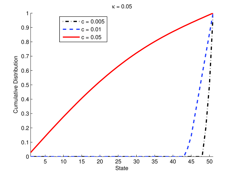
9.2 Comparative Statics: Marginal Cost

Figure 1 plots the cumulative distribution function of the mean field equilibrium population state for $\kappa=0.05$ and for different values of the marginal cost $c$ at the end of the $1000$-th iteration. Observe that as the marginal cost increases from $c=0.005$ to $c=0.05$, the mass of the equilibrium population state shifts to lower security levels. This is as predicted by Theorem 5.1: at a higher marginal cost, it is costly to maintain a higher security level, and hence players tend to invest less— resulting in an equilibrium distribution with substantial weight at lower states. Note that even small changes in the marginal cost can significantly shift the equilibrium profile.

Figure 2: Cumulative distribution function of population state at $t=1000$ under L-MLD for $\kappa=0.05$ and marginal cost $c=0.05$, with different distributions for $W$. In all cases $q_{0}=0.2$. The solid line is for $q_{-1}=q_{1}=0.4$; the dashed line is for $q_{-1}=0.45,q_{1}=0.35$; and the dashed dotted line is for $q_{-1}=0.5,q_{1}=0.3$.

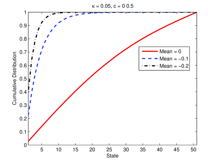
9.3 Comparative Statics: Transition Kernel

Figure 2 plots a different kind of comparative statics result, where we plot the cumulative distribution function of the mean field equilibrium population state for different noise distributions. We observe that as the mean of the noise distribution becomes negative, the equilibrium distribution tends to concentrate over lower states. One can interpret this negative mean as the tendency of the player’s security to deteriorate over time, e.g., because the anti-virus software installed on a machine becomes outdated. Thus, each player needs to constantly take an action to maintain its security level. For a fixed marginal cost of action, a more negative drift results in players moving toward lower security levels. Note that even for small negative drift in the noise distribution, the cumulative distribution rapidly concentrates over lower states. Thus in order to maintain a desired security level in a network, a network administrator should try to ensure that an individual player’s security level does not depreciate quickly over time.

9.4 Heterogeneity

We now consider a model where players may be heterogeneous. Specifically, we consider two types of players whose payoff function is parameterized by an interaction parameter $\delta$. This interaction parameter controls the effect of the security level of other players on the payoff of an individual player. The payoff function is then given by:

$$\pi\left(x,a,f;\delta\right)=-p(x)-\delta(1-p(x))\eta(f)-ca,$$

where $\eta(f)$ is the mean of $f$. A higher value of $\delta$ implies that a player frequently interacts with other players in the network. Thus, the average security level of other players has a higher impact on its own security. As discussed in the conclusion, all the results of our paper continue to apply for a model with heterogeneous players.

For the purposes of this numerical example, we consider two values of the interaction parameter—a low value given by $\delta_{L}=0.1$ and a high value given by $\delta_{H}=0.9$. Figure 3 plots the mean of the mean field equilibrium population state as the fraction of players with lower $\delta$ increases. When all players have a high interaction parameter, they interact with each other more often. Hence each player has a high probability of a bad event, and so feels that a personal investment in security is not likely to be particularly productive. A “tragedy of the commons” ensues, and the resulting mean population state is quite low in equilibrium. On the other hand, even for a small fraction of players with the low interaction parameter, the mean security level of all players increases. This is because those players feel a positive benefit to investing their own security level, and thus encourage others to invest as well—even those with the high interaction parameter. Thus in a real network, slightly limiting interaction between players can have a significant impact on the overall security level of the system.

Figure 3: Mean of the mean field equilibrium population state vs. the fraction of players with low interaction parameter, i.e., $\delta=\delta_{L}$. Here $\kappa=0.05$ and $c=0.05$.

Figure 4: Total variation distance between the actual distribution and the empirical distribution for L-MLD with $m=50$ and L-MLD with $m=1000$ players. Here $\kappa=0.05$ and $c=0.05$.

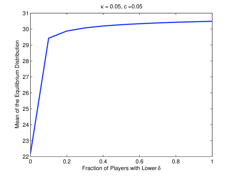
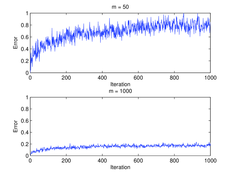
9.5 Convergence of L-MLD: Finite vs. Mean Field

As noted above, the mean field equilibrium is computed using L-MLD. In such dynamics, agents compute their current optimal strategy assuming that the population state remains fixed for all future time. Using this computed optimal strategy, the next population state is computed using equation (13). This process is repeated until convergence. In this computation, the next population state is a deterministic function of the previous distribution, and it depends on the optimal strategy via the transition kernel; this is a consequence of the mean field limit.

Here we ask the question: what happens if finitely many players use L-MLD? In other words, each player $i$ in a game with $m$ players observes the true population state at time $t$, $f_{-i,t}^{(m)}$; and then executes L-MLD with respect to this population state. Errors are then introduced because the next population state is stochastic in a finite system. (See discussion at the end of Section 4.)

In Figure 4, we plot the total variation error between successive population states, for $m=50$ and $m=1000$ players. As we observe, for a small number of players ($m=50$), the error can be high, and accumulates as time passes. However, for a large number of players ($m=1000$), this error is considerably reduced.

This effect is also seen in the limiting population state. In Figure 5, we plot the cumulative distribution function at $t=1000$ for three cases: the mean field L-MLD; L-MLD with $m=50$ players; and L-MLD with $m=1000$ players. As we observe, for $m=1000$, the population state is very close to the population state obtained using the mean field deterministic update (cf. (13)).

Figure 5: Cumulative distribution function of the population state at $t=1000$ under L-MLD for $\kappa=0.05$ and marginal cost $c=0.05$. The plot includes the population state obtained under the deterministic mean field L-MLD; L-MLD with $m=50$ players; and L-MLD with $m=1000$ players.

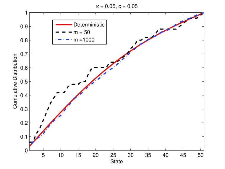
10 Conclusion

This paper has considered existence of mean field equilibrium in games that exhibit strategic complementarities in the states of the players. Our proofs exploit monotonicity and complementarity properties of the model primitives to demonstrate that there exist both a “largest” and “smallest” mean field equilibrium among all equilibria where the strategy is nondecreasing in the state. Further, we demonstrate that there exist natural myopic learning dynamics that converge to these equilibria. Finally, we apply our results in the context and illustrate how specific examples of games with complementarities may be analyzed using our techniques.

We conclude by noting two extensions that can be developed for the models described here.

1. Types. In our model players are homogeneous; however, this is not a consequential restriction, and is made primarily for convenience. In Section 9.4, we considered a numerical example with heterogeneous players. More generally, we can extend the definition of a stochastic game by assuming that there exists a finite type space $\Delta$, with $\pi(x,a,f;\delta)$ and $\mathbf{P}(\cdot|x,a,f;\delta)$ the payoff and transition kernel, respectively, of a type $\delta$ player. Further, we assume that the probability a player is of type $\delta$ is given by $\psi(\delta)$. With this extension, as long as the conditions of Definition 3.1 are satisfied for each $\delta$, it is straightforward to extend our existence, convergence, and comparative statics results. The main technical issue is that now a mean field equilibrium must provide an optimal strategy $\mu_{\delta}$ and population state $f_{\delta}$ for each $\delta$. We omit the details.

2. Multidimensional state and action spaces. A more difficult extension involves models where the state and action spaces may be multidimensional lattices. The main challenge here arises because the set of distributions on a multidimensional compact lattice $\mathcal{X}$ is not generally a lattice in the first order stochastic dominance ordering; see Kamae et al. (1977) for details. However, first order stochastic dominance does give a closed partial order on the set of distributions on $\mathcal{X}$.

   We can leverage this fact as follows. Suppose that in addition to the conditions of Definition 3.1, the action set is a fixed lattice $\mathcal{A}$ for all $x$, i.e., $\mathcal{A}(x)=\mathcal{A}$ for all $x$. Further, suppose the model primitives (payoff and transition kernel) are all continuous in state, action, and population state—i.e., Assumption 4.1 is satisfied. Then Kleene’s fixed point theorem (Kleene 1971) can be used to establish existence of, and convergence to, a mean field equilibrium. Kleene’s fixed point theorem states that if $X$ is a space with a closed partial order and a smallest element, then any monotone continuous function from $X$ to itself possesses a fixed point. We omit the details of this argument, as it is essentially identical to our preceding development.

   We do emphasize, however, that our analysis of separable stochastic games is intimately tied to the assumption that state and action spaces are single-dimensional. In particular, our proof techniques rely heavily on the scalar nature of the action and kernel parameter spaces (cf. Lemma 7.4); relaxing these conditions remains an open direction.

11 Proofs: Section 3.1

We start with the lemma that demonstrates that optimal strategies exist, and can be identified via Bellman’s equation; the proof uses standard results from dynamic programming.

Lemma 11.1

For each $f\in\mathfrak{F}$, $\mathcal{P}(f)$ is nonempty. Furthermore, $\mu\in\mathcal{P}(f)$ if and only if for each $x$:

$$\mu(x)\in\arg\max_{a\in\mathcal{A}(x)}\left\{\pi(x,a,f)+\beta\int_{\mathcal{X}}V^{*}(x^{\prime}|f)\mathbb{P}(dx^{\prime}|x,a,f)\right\}$$

Proof 11.2

Proof. Throughout the proof we employ Definition 3.1. In particular, observe that the payoff is continuous on a compact set $\mathsf{A}$ and thus for fixed $f$, the payoff $\pi(x,a,f)$ is bounded. In addition, for each fixed $x$, the next state is drawn from a countable set by assumption. Thus consider maximization of the expected discounted profit over all possible (randomized, history-dependent) strategies; by standard results in the theory of dynamic programming (see Bertsekas and Shreve 1978), it can be shown that if there exists an optimal strategy, there must exist an optimal stationary, nonrandomized, Markov strategy—i.e., in our terminology, an oblivious strategy. Further, $V^{*}$ satisfies Bellman’s equation:

$$V^{*}(x|f)=\sup_{a\in\mathcal{A}(x)}\left\{\pi(x,a,f)+\beta\int_{\mathcal{X}}V^{*}(x^{\prime}|f)\mathbb{P}(dx^{\prime}|x,a,f)\right\};$$ (21)

and an oblivious strategy is optimal if and only if it attains the maximum on the right hand side of the preceding expression for every $x$.

Observe also that for fixed $f$, $V^{*}(\cdot|f)$ is bounded, since the per stage payoffs are bounded and the discount factor is less than one. Since the transition probability $\mathbb{P}(\cdot|x,a,f)$ is continuous w.r.t. the topology of weak convergence, we conclude the objective function in (21) is continuous in $a$. Because $\mathcal{A}(x)$ is compact, the maximum is achieved for every $x$, and thus at least one optimal strategy must exist—i.e., $\mathcal{P}(f)$ is nonempty. This proves the lemma.

The next three lemmas combine to show that the value function $V^{*}(x|f)$ has increasing differences in $x$ and $f$.

Lemma 11.3

Suppose that $U(x|f)$ is a nondecreasing bounded function in $x$ and has increasing differences in $x$ and $f$. Define

$$T(x,a,f)=\int_{\mathcal{X}}U(x^{\prime}|f)\mathbb{P}(dx^{\prime}|x,a,f).$$ (22)

Then $T(x,a,f)$ is nondecreasing in $x$ and $a$, supermodular in $(x,a)$ and has increasing differences in $(x,a)$ and $f$.

Proof 11.4

Proof. By Definition 3.1, $\mathbb{P}\left(\cdot|x,a,f\right)$ is stochastically nondecreasing in $x$ and $a$ and stochastically supermodular in $(x,a)$. Since $U(x|f)$ is a nondecreasing bounded function, it follows from the definition of stochastically nondecreasing and stochastically supermodular that $T(x,a,f)$ is nondecreasing in $x$ and $a$ and supermodular in $(x,a)$ for fixed $f$.

Fix $\hat{x}\geq x$, $\hat{a}\geq a$, and $\hat{f}\succeq_{\mathsf{SD}}f$ and define

$$\hat{T}(x,a,f,g)=\int_{\mathcal{X}}U(x|f)\mathbb{P}(dx|x,a,g).$$

To prove $T(x,a,f)$ has increasing differences in $(x,a)$ and $f$, it suffices to show that

$$\hat{T}(\hat{x},\hat{a},\hat{f},\hat{f})-\hat{T}(x,a,\hat{f},\hat{f})\geq\hat{T}(\hat{x},\hat{a},f,f)-\hat{T}(x,a,f,f).$$ (23)

Let us fix $g$; since $U(x|f)$ has increasing differences in $x$ and $f$, $U(x|\hat{f})-U(x|f)$ is a nondecreasing function of $x$. Since $\mathbb{P}(\cdot|\hat{x},a,g)\succeq_{\mathsf{SD}}\mathbb{P}(\cdot|x,a,g)$ by Definition 3.1, it follows that:

$$\hat{T}(\hat{x},a,\hat{f},g)-\hat{T}(\hat{x},a,f,g)\geq\hat{T}(x,a,\hat{f},g)-\hat{T}(x,a,f,g).$$ (24)

Also by Definition 3.1, $\mathbb{P}(\cdot|\hat{x},\hat{a},g)\succeq_{\mathsf{SD}}\mathbb{P}(\cdot|\hat{x},a,g)$ which implies that

$$\hat{T}(\hat{x},\hat{a},\hat{f},g)-\hat{T}(\hat{x},\hat{a},f,g)\geq\hat{T}(\hat{x},a,\hat{f},g)-\hat{T}(\hat{x},a,f,g).$$ (25)

Using equations (24) and (25) and rearranging the terms, we get that

$$\hat{T}(\hat{x},\hat{a},\hat{f},g)-\hat{T}(x,a,\hat{f},g)\geq\hat{T}(\hat{x},\hat{a},f,g)-\hat{T}(x,a,f,g).$$ (26)

Now let $\hat{g}\succeq_{\mathsf{SD}}g$ and note that $\mathbb{P}(\cdot|x,a,g)$ has increasing differences in $(x,a)$ and $g$ by Definition 3.1. Also, note that $U(x|f)$ is a bounded nondecreasing function of $x$. This implies that $\hat{T}(x,a,f,g)$ has increasing differences in $(x,a)$ and $g$. That is,

$$\hat{T}(\hat{x},\hat{a},\hat{f},\hat{g})-\hat{T}(x,a,\hat{f},\hat{g})\geq\hat{T}(\hat{x},\hat{a},\hat{f},g)-\hat{T}(x,a,\hat{f},g).$$ (27)

From equations (26) and (27), we get that for any $\hat{x}\geq x$, $\hat{a}\geq a$, $\hat{f}\succeq_{\mathsf{SD}}f$, and $\hat{g}\succeq_{\mathsf{SD}}g$ we have

$$\hat{T}(\hat{x},\hat{a},\hat{f},\hat{g})-\hat{T}(x,a,\hat{f},\hat{g})\geq\hat{T}(\hat{x},\hat{a},f,g)-\hat{T}(x,a,f,g).$$

Taking $\hat{f}=\hat{g}$ and $f=g$ in the above equation shows that equation (23) is true which proves the lemma.

Lemma 11.5

Suppose that $U(x|f)$ is a nondecreasing bounded function in $x$ that has increasing differences in $x$ and $f$. Define

$$U^{*}(x|f)=\sup_{a\in\mathcal{A}(x)}\left\{\pi(x,a,f)+\beta\int_{\mathcal{X}}U(x^{\prime}|f)\mathbb{P}\left(dx^{\prime}|x,a,f\right)\right\}.$$

Then $U^{*}(x|f)$ is nondecreasing in $x$ and has increasing differences in $x$ and $f$.

Proof 11.6

Proof. Define

$$W(x,a,f) =\pi(x,a,f)+\beta\int_{\mathcal{X}}U(x^{\prime}|f)\mathbb{P}\left(dx^{\prime}|x,a,f\right)$$

$$=\pi(x,a,f)+\beta T(x,a,f).$$

From Lemma 11.3, we know that $T(x,a,f)$ is nondecreasing in $x$ and $a$, supermodular in $(x,a)$ and has increasing differences in $(x,a)$ and $f$. From Definition 3.1, we get that $W(x,a,f)$ is nondecreasing in $x$, supermodular in $(x,a)$ and has increasing differences in $(x,a)$ and $f$.

We now show that $U^{*}(x|f)$ is nondecreasing in $x$ for fixed $f$. Fix $x^{\prime}\geq x$, and choose $\hat{a}\in\mathcal{A}(x)$ such that $W(x,\hat{a},f)=\sup_{a\in\mathcal{A}(x)}W(x,a,f)$; such an action exists since $\pi$ and $\mathbb{P}$ are continuous in $a$ and $\mathcal{A}(x)$ is compact. Similarly, fix $\hat{a}^{\prime}$ such that $\pi(x,\hat{a}^{\prime},f)=\sup_{a\in\mathcal{A}(x^{\prime})}\pi(x,a,f)$.

We consider two cases. If $\hat{a}\in\mathcal{A}(x^{\prime})$, then:

$$U^{*}(x|f) =\pi(x,\hat{a},f)+\beta T(x,\hat{a},f)$$

$$\leq\pi(x^{\prime},\hat{a},f)+\beta T(x^{\prime},\hat{a},f)$$

$$\leq\sup_{a\in\mathcal{A}(x^{\prime})}\pi(x^{\prime},a,f)+\beta T(x^{\prime},a,f)=U^{*}(x^{\prime}|f),$$

where the first inequality follows since $\pi$ and $T$ are both nondecreasing in $x$.

On the other hand, if $\hat{a}\not\in\mathcal{A}(x^{\prime})$, then it follows that $\hat{a}^{\prime}>\hat{a}$, since $\mathcal{A}$ is a nondecreasing correspondence. (Note that this step uses the fact that the action set is totally ordered.) Thus:

$$U^{*}(x|f) =\pi(x,\hat{a},f)+\beta T(x,\hat{a},f)$$

$$\leq\pi(x^{\prime},\hat{a}^{\prime},f)+\beta T(x,\hat{a},f)$$

$$\leq\pi(x^{\prime},\hat{a}^{\prime},f)+\beta T(x^{\prime},\hat{a}^{\prime},f)$$

$$\leq\sup_{a\in\mathcal{A}(x^{\prime})}\pi(x^{\prime},a,f)+\beta T(x^{\prime},a,f)=U^{*}(x^{\prime}|f),$$

Here the first inequality follows since $\sup_{a\in\mathcal{A}(x)}\pi(x,a,f)$ is nondecreasing in $x$, and by our choice of $\hat{a}^{\prime}$; and the second inequality follows since $T$ is nondecreasing in $x$ and $a$. We conclude that $U^{*}(x|f)$ is nondecreasing in $x$ for fixed $f$.

To prove that $U^{*}(x|f)$ has increasing differences, we reason using an argument similar to Lemma $A.1$ of Hopenhayn and Prescott (1992). Let $x_{2}\geq x_{1}$ and $f_{2}\succeq_{\mathsf{SD}}f_{1}$. To prove that $U^{*}(x|f)$ has increasing differences, we need to show that

$$U^{*}(x_{2}|f_{2})-U^{*}(x_{1}|f_{2})\geq U^{*}(x_{2}|f_{1})-U^{*}(x_{1}|f_{1}).$$ (28)

To economize on notation, given two actions $a,a^{\prime}$, we let $a\vee a^{\prime}=\sup\{a,a^{\prime}\}$, and let $a\wedge a^{\prime}=\inf\{a,a^{\prime}\}$. Fix $a_{1}\in\mathcal{A}(x_{1})$ and $a_{2}\in\mathcal{A}(x_{2})$. Since $\mathcal{A}(x)$ is a nondecreasing correspondence, we have $a_{1}\vee a_{2}\in\mathcal{A}(x_{2})$ and $a_{1}\wedge a_{2}\in\mathcal{A}(x_{1})$. Thus we have:

$$U^{*}(x_{1}|f_{1})+U^{*}(x_{2}|f_{2}) \geq W(x_{1},a_{1}\wedge a_{2},f_{1})+W(x_{2},a_{1}\vee a_{2},f_{2})$$

$$=W(x_{1},a_{1}\wedge a_{2},f_{1})+W(x_{2},a_{1}\vee a_{2},f_{2})+W(x_{1},a_{1}\wedge a_{2},f_{2})$$

$$\quad\quad\quad-W(x_{1},a_{1}\wedge a_{2},f_{2})$$

$$=W(x_{1},a_{1}\wedge a_{2},f_{1})+W(x_{1}\vee x_{2},a_{1}\vee a_{2},f_{2})+W(x_{1}\wedge x_{2},a_{1}\wedge a_{2},f_{2})$$

$$\quad\quad-W(x_{1},a_{1}\wedge a_{2},f_{2})$$

The last equality follows from that fact that $x_{1}\vee x_{2}=x_{2}$ and $x_{1}\wedge x_{2}=x_{1}$. Since $W(x,a,f)$ is supermodular in $(x,a)$ we get that

$$U^{*}(x_{1}|f_{1})+U^{*}(x_{2}|f_{2}) \geq W(x_{1},a_{1}\wedge a_{2},f_{1})+W(x_{2},a_{2},f_{2})+W(x_{1},a_{1},f_{2})$$

$$\quad\quad\quad-W(x_{1},a_{1}\wedge a_{2},f_{2}),$$

$$=W(x_{1},a_{1},f_{2})+W(x_{2},a_{2},f_{1})-W(x_{2},a_{2},f_{1})+W(x_{2},a_{2},f_{2})$$

$$\quad\quad\quad+W(x_{1},a_{1}\wedge a_{2},f_{1})-W(x_{1},a_{1}\wedge a_{2},f_{2})$$

$$\geq W(x_{1},a_{1},f_{2})+W(x_{2},a_{2},f_{1}).$$

Here the last inequality follows from the fact that $W(x,a,f)$ has increasing differences in $(x,a)$ and $f$. Taking the supremum over $a_{1}$ and $a_{2}$ in the above inequality we get

$$U^{*}(x_{1}|f_{1})+U^{*}(x_{2}|f_{2}) \geq U^{*}(x_{1}|f_{2})+U^{*}(x_{2}|f_{1})$$

which implies equation (28), and thus $U^{*}(x|f)$ has increasing differences in $x$ and $f$. This proves the lemma.

Lemma 11.7

$V^{*}(x|f)$ is nondecreasing in $x$ and has increasing differences in $x$ and $f$.

Proof 11.8

Proof. Let $V_{0}(x|f)=0$ for all $x$, and let:

$$V_{k+1}(x|f)=\sup_{a\in\mathcal{A}(x)}\left\{\pi(x,a,f)+\beta\int_{\mathcal{X}}V_{k}(x^{\prime}|f)\mathbb{P}(dx^{\prime}|x,a,f)\right\};$$ (29)

this is value iteration. By the preceding lemma, every $V_{k}$ is nondecreasing in $x$ and has increasing differences in $x$ and $f$. Under our assumptions, value iteration converges starting from the zero function (Bertsekas 2001), i.e., for all $x$, $V_{k}(x|f)\to V^{*}(x|f)$ as $k\to\infty$. Since monotonicity and increasing differences are preserved upon taking limits, we conclude $V^{*}(x|f)$ is nondecreasing in $x$ and has increasing differences in $x$ and $f$.

We now apply Topkis’ Theorem in the next lemma to conclude the set of optimal strategies is monotone.

Lemma 11.9

For each $x$ and $f$, define the set $\Omega(x,f)$ as:

$$\Omega(x,f)=\arg\max_{a\in\mathcal{A}(x)}\left\{\pi(x,a,f)+\beta\int_{\mathcal{X}}V^{*}(x^{\prime}|f)\mathbb{P}(dx^{\prime}|x,a,f)\right\}.$$ (30)

Then $\Omega$ is nondecreasing in $(x,f)$.

Further:

$$\overline{p}(f)(x)=\sup\Omega(x,f);\ \ \underline{p}(f)(x)=\inf\Omega(x,f),$$

where $\overline{p}$ and $\underline{p}$ are the strategies defined in (9). Both $\overline{p}(f)$ are $\underline{p}(f)$ are nondecreasing in $f$, and for fixed $f$ both strategies are also nondecreasing in $x$.

Proof 11.10

Proof. Observe that $\pi(x,a,f)$ is supermodular in $(x,a)$ and has increasing differences in $(x,a)$ and $f$ (by Definition 3.1); and $T(x,a,f)$ is supermodular in $(x,a)$ and has increasing differences in $(x,a)$ and $f$, where $T$ is defined in equation (22), with $U=V^{*}$ (by Lemma 11.3 and 11.7). Further, $\mathcal{A}(x)$ is an increasing correspondence. By Topkis’ Theorem (Theorem 2.8.1 in Topkis 1998), we conclude that $\Omega(x,f)$ is nondecreasing in $(x,f)$ wherever it is nonempty. By Lemma 11.1, however, the maximum on the right hand side in (30) is always achieved, so $\Omega(x,f)$ is nondecreasing everywhere.

To conclude the proof, observe that by Lemma 11.1, $\overline{p}(f)$ must be the strategy that takes the largest action in $\Omega(x,f)$ for each $x$, and $\underline{p}(f)$ must be the strategy that takes the smallest action in $\Omega(x,f)$ for each $x$. Monotonicity of $\overline{p}$ and $\underline{p}$ follows from the monotonicity properties of $\Omega$.

We now turn our attention to $\mathcal{D}$. Given any strategy $\mu$ and population state $f$, define a map $Q_{\mu,f}:\mathfrak{F}\rightarrow\mathfrak{F}$ according to the kernel induced by $\mu$ and $f$, i.e., for all Borel sets S:

$$Q_{\mu,f}(g)(S)=\int_{\mathcal{X}}\mathbb{P}(S|x,\mu(x),f)\;g(dx).$$

(This is equation (14).)

Lemma 11.11

Suppose $f^{\prime}\succeq_{\mathsf{SD}}f$, $g^{\prime}\succeq_{\mathsf{SD}}g$, and $\mu^{\prime}\unrhd\mu$, and both $\mu^{\prime}$ and $\mu$ are nondecreasing, then $Q_{\mu^{\prime},f^{\prime}}(g^{\prime})\succeq_{\mathsf{SD}}Q_{\mu,f}(g)$.

Proof 11.12

Proof. Let $\phi$ be a bounded nondecreasing real-valued function on $\mathcal{X}$. We need to show that for every $x\in\mathcal{X}$, we have

$$\int_{\mathcal{X}}\int_{\mathcal{X}}\phi(y)\mathbb{P}\left(dy|x,\mu^{\prime}(x),f^{\prime}\right)g^{\prime}(dx)\geq\int_{\mathcal{X}}\int_{\mathcal{X}}\phi(y)\mathbb{P}\left(dy|x,\mu(x),f\right)g(dx).$$ (31)

Let us define

$$H(x;\mu,f)=\int_{\mathcal{X}}\phi(y)\;\mathbb{P}(dy|x,\mu(x),f).$$

Observe that:

$$\int_{\mathcal{X}}\int_{\mathcal{X}}\phi(y)\mathbb{P}(dy|x,\mu(x),f)\;g(dx)=\int_{\mathcal{X}}H(x;\mu,f)\;g(dx).$$

Let $x^{\prime}\geq x$ and note that $\mu$ is a nondecreasing function of $x$. From Definition 3.1, we know that $\mathbb{P}(\cdot|x,a,f)$ is stochastically nondecreasing in $(x,a)$, which implies that $\mathbb{P}(\cdot|x^{\prime},\mu(x^{\prime}),f)\succeq_{\mathsf{SD}}\mathbb{P}(\cdot|x,\mu(x),f)$. Since $\phi$ is a nondecreasing function, we get that $H(x^{\prime};\mu,f)\geq H(x;\mu,f)$.

From Definition 3.1, we know that $\mathbb{P}(\cdot|x,a,f)$ is nondecreasing in $a$ and $f$. Thus, for any fixed $x$, we have

$$\mathbb{P}(\cdot|x,\mu^{\prime}(x),f^{\prime})\succeq_{\mathsf{SD}}\mathbb{P}(\cdot|x,\mu(x),f).$$

This along with the fact that $\phi$ is a nondecreasing function implies that $H(x;\mu^{\prime},f^{\prime})\geq H(x;\mu,f)$ for every fixed $x\in\mathcal{X}$.

We now reason as follows:

$$\int_{\mathcal{X}}H(x;\mu^{\prime},f^{\prime})g^{\prime}(dx) \geq\int_{\mathcal{X}}H(x;\mu,f)g^{\prime}(dx)$$

$$\geq\int_{\mathcal{X}}H(x;\mu,f)g(dx).$$

Here the first inequality follows from the fact that $H(x;\mu^{\prime},f^{\prime})\geq H(x;\mu,f)$ and the second inequality follows from that fact that $H(x^{\prime};\mu,f)\geq H(x;\mu,f)$ for $x^{\prime}\geq x$, and that $g^{\prime}\succeq_{\mathsf{SD}}g$. This proves equation (31) and hence proves the lemma.

Lemma 11.13

Fix $\mu\in\mathfrak{M}_{O}$ and $f\in\mathfrak{F}$, and suppose $\mu$ is nondecreasing in $x$. Then $\mathcal{D}(\mu,f)$ is a nonempty complete lattice. Further, $\underline{d}(\mu,f)$ and $\overline{d}(\mu,f)$ (as defined in (10)) exist and are both invariant distributions of the Markov process induced by $\mu$ and $f$ (cf. (7)).

Finally, if $f^{\prime}\succeq_{\mathsf{SD}}f$ and $\mu^{\prime}\unrhd\mu$ and both $\mu$ and $\mu^{\prime}$ are nondecreasing, then $\underline{d}(\mu^{\prime},f^{\prime})\succeq_{\mathsf{SD}}\underline{d}(\mu,f)$ and $\overline{d}(\mu^{\prime},f^{\prime})\succeq_{\mathsf{SD}}\overline{d}(\mu,f)$.

Proof 11.14

Proof. By the preceding lemma, $Q_{\mu,f}(g)$ is nondecreasing in $g$. By Tarski’s theorem, the set of fixed points of $Q_{\mu,f}$ is a nonempty complete lattice. View the set of nondecreasing strategies $\mu$ as a partially ordered set $\mathfrak{M}_{O}$, with the coordinate-wise ordering $\unrhd$. Then $Q_{\mu,f}(\cdot)$ is a nondecreasing function on $\mathfrak{M}_{O}\times\mathfrak{F}\times\mathfrak{F}$, by the preceding lemma. Theorem 2.5.2 in Topkis (1998) generalizes Tarski’s theorem to fixed points of a nondecreasing function parametrized by a partially ordered set ($\mathfrak{M}_{O}\times\mathfrak{F}$); one consequence of this generalization is that the largest and smallest fixed points are nondecreasing in the parameter. This generalization directly implies that both $\underline{d}(\mu,f)$ and $\overline{d}(\mu,f)$ are nondecreasing in $\mu$ and $f$.

In the next lemma we establish existence of fixed points of $\Phi$, thus proving Theorem 3.4.

Lemma 11.15

Let $\underline{\Phi}(f)$ and $\overline{\Phi}(f)$ be defined as in (11). Then $\underline{\Phi}(f),\overline{\Phi}(f)\in\Phi(f)$. Further, both are nondecreasing in $f$, and thus the sets of their fixed points are each nonempty complete lattices.

Thus there exists a mean field equilibrium for the stochastic game with complementarities $\Gamma$: in particular, if $f$ is a fixed point of $\underline{\Phi}$ (resp., $\overline{\Phi}$), then $(\underline{p}(f),f)$ (resp., $(\overline{p}(f),f)$) is a mean field equilibrium.

Proof 11.16

Proof. That $\Phi(f)$ is nonempty follows by Lemmas 11.1 and 11.13. Observe that if $f^{\prime}\succeq_{\mathsf{SD}}f$, then $\underline{p}(f^{\prime})\unrhd\underline{p}(f)$ by Lemma 11.9. Further, $\underline{p}(f^{\prime})$ and $\underline{p}(f)$ are both nondecreasing in $x$ as well, so by Lemma 11.13, $\underline{d}(\underline{p}(f^{\prime}),f^{\prime})\succeq_{\mathsf{SD}}\underline{d}(\underline{p}(f),f)$, establishing that $\underline{\Phi}$ is monotone. That $\underline{\Phi}(f)\in\Phi(f)$ follows from the definition. The proof for $\overline{\Phi}(f)$ is identical. The conclusion regarding fixed points follows from Tarski’s theorem.

12 Proofs: Section 3.2

Proof 12.1

Proof of Corollary 3.5. Since $\overline{p}(f)=\sup\mathcal{P}(f)$, and $\mu\in\mathcal{P}(f)$, we must have $\overline{p}(f)\unrhd\mu$. Similarly $\mu\unrhd\underline{p}(f)$. Now since $\overline{p}(f)$ and $\underline{p}(f)$ are both nondecreasing strategies, by Lemma 11.13 we conclude that $\overline{\Phi}(f)=\overline{d}(\overline{p}(f),f)\succeq_{\mathsf{SD}}\overline{d}(\mu,f)\succeq_{\mathsf{SD}}f$, where the last inequality follows because $\overline{d}(\mu,f)=\sup\mathcal{D}(\mu,f)$, and $f\in\mathcal{D}(\mu,f)$. A similar argument shows that $f\succeq_{\mathsf{SD}}\underline{\Phi}(f)$. The result now follows from Theorem 2.5.1 in Topkis (1998), which is a sharper version of Tarski’s fixed point theorem; in particular, that statement shows that $\overline{f}=\sup\{f^{\prime}:\overline{\Phi}(f)\succeq_{\mathsf{SD}}f\}$, and $\underline{f}=\inf\{f^{\prime}:f\succeq_{\mathsf{SD}}\underline{\Phi}(f)\}$. Since $f$ is contained in both the former and the latter sets, we conclude $\underline{f}\preceq_{\mathsf{SD}}f\preceq_{\mathsf{SD}}\overline{f}$. The result regarding strategies now follows from monotonicity of $\underline{p}$ and $\overline{p}$, and the fact that $\underline{p}(f)\unlhd\mu\overline{p}(f)$.

13 Proofs: Section 4

We start with two essential lemmas.

Lemma 13.1

Suppose that $f_{0}\preceq_{\mathsf{SD}}f_{1}\preceq_{\mathsf{SD}}f_{2}\cdots$, and $\mu_{0}\unlhd\mu_{1}\unlhd\mu_{2}\cdots$. Then there exists a distribution $f^{*}$ and a strategy $\mu^{*}$ such that $f_{t}$ converges weakly to $f^{*}$ as $t\to\infty$, and $\mu_{t}$ converges pointwise to $\mu^{*}$ as $t\to\infty$.

Proof 13.2

Proof. Note that since the set $\mathfrak{M}_{O}$ is compact and $\mu_{t}$ is a nondecreasing sequence of policies, there must exist a pointwise limit $\mu^{*}$. Next, consider the distribution functions $F_{t}$ corresponding to the measures $f_{t}$. By Prohorov’s theorem, there exists a measure $f^{*}\in\mathfrak{F}$ and a subsequence $t_{k}$ such that $F_{t_{k}}(x)\to F^{*}(x)$ at all points of continuity of $F^{*}$, where $F^{*}$ is the distribution function corresponding to $f^{*}$. Since $f_{t}$ is a monotone sequence, we have $F_{t}(x)\geq F_{t+1}(x)$ for all $x$, so in fact $F_{t}(x)\to F^{*}(x)$ at all points of continuity of $F^{*}$. Thus $f_{t}$ converges weakly to $f^{*}$, as required.

Lemma 13.3

Suppose Assumption 4.1 holds. Then $\underline{p}(f)$ and $\overline{p}(f)$ (cf. (9)) are both continuous in $f$, and $Q_{\mu,g}(f)$ (cf. (14)) is continuous in $\mu$, $g$, and $f$, where we endow $\mathfrak{F}$ with the topology of weak convergence, and $\mathfrak{M}_{O}$ with the topology of pointwise convergence.

Proof 13.4

Proof. Under Assumption 4.1, the first result follows using Theorem 1 of Dutta et al. (1994), which establishes upper semicontinuity of $\Omega(x,f)$ in $f$ (where $\Omega$ is defined as in (30)). From this it follows that $\underline{p}(f)$ and $\overline{p}(f)$ are continuous in $f$.

Next we show that $Q_{\mu,g}(f)$ as defined in (14) is continuous in $\mu$, $g$ and $f$, where we endow $\mathfrak{F}$ with the topology of weak convergence, and $\mathfrak{M}_{O}$ with the topology of pointwise convergence. Suppose that $g_{n}\to g$ (weakly), $f_{n}\to f$ (weakly), and that $\mu_{n}\to\mu$ (pointwise). Fix a bounded function $\phi$ on $\mathcal{X}$, and define

$$H(x;\mu,g)=\int_{\mathcal{X}}\phi(y)\mathbf{P}(dy|x,\mu(x),g).$$

For every $x$, $H(x;\mu_{n},g_{n})\to H(x;\mu,g)$ by continuity of $\mathbf{P}(\cdot|x,a,g)$ in $a$ and $g$. Thus by Theorem 5.5 of Billingsley (1968), we have:

$$\int_{\mathcal{X}}H(x;\mu_{n},g_{n})f_{n}(dx)\to\int_{\mathcal{X}}H(x;\mu,g)f(dx).$$

The left hand side is the expected value of $\phi$ under $Q_{\mu_{n},g_{n}}(f_{n})$, and the right hand side is the expected value of $\phi$ under $Q_{\mu,g}(f)$, so (weak) continuity of $Q_{\mu,g}(f)$ is proved.

Proof 13.5

Proof of Proposition 4.1. Since $f_{t+1}=\underline{\Phi}(f_{t})$, and $\underline{\Phi}$ is monotone by Lemma 11.15, it follows that $f_{0}\preceq_{\mathsf{SD}}f_{1}\preceq_{\mathsf{SD}}f_{2}\cdots$. Since $\mu_{t}=\underline{p}(f_{t})$, and $\underline{p}$ is monotone in $f_{t}$ by Lemma 11.9, it follows that $\mu_{0}\unlhd\mu_{1}\unlhd\mu_{2}\cdots$. Finally, since $\underline{p}(f)(x)$ is nondecreasing in $x$ for every $f$, it follows that $\mu_{t}$ is nondecreasing. By Lemma 13.1, there exists a limit $(\mu^{*},f^{*})$. Since every $\mu_{t}$ is nondecreasing in $x$, the limit $\mu^{*}$ must be nondecreasing in $x$ as well.

We now show that if Assumption 4.1 holds, then the limit point $(\mu^{*},f^{*})$ is the smallest mean field equilibrium. By Lemma 13.3, both $\underline{p}(f)$ and $Q_{\mu,g}(f)$ are continuous. This implies that $\mu_{t}=\underline{p}(f_{t})\to\underline{p}(f^{*})$ as $t\to\infty$, so $\mu^{*}=\underline{p}(f^{*})$. Further, since $f_{t+1}=\underline{d}(\mu_{t},f_{t})$, it follows that $Q_{\mu_{t},f_{t}}(f_{t+1})=f_{t+1}$. Taking limits on the left and right, we have $Q_{\mu^{*},f^{*}}(f^{*})=f^{*}$, i.e., $f^{*}\in\mathcal{D}(\mu^{*},f^{*})$. Thus we conclude $(\mu^{*},f^{*})$ is a mean field equilibrium.

Let $\underline{f}$ be the smallest fixed point of $\underline{\Phi}(f)$, as defined in (12). Observe that at time 0, $f_{0}\preceq_{\mathsf{SD}}\underline{f}$, since $f_{0}$ is the smallest distribution in the lattice $\mathfrak{F}$. Since $\Phi$ is monotone, $f_{t}\preceq_{\mathsf{SD}}\underline{f}$ for all $t$. Since $f_{t}$ converges weakly to $f^{*}$, we conclude $f^{*}\preceq_{\mathsf{SD}}\underline{f}$. On the other hand, observe that $\mu^{*}$ is nondecreasing, so by Corollary 3.5, we have $\underline{f}\preceq_{\mathsf{SD}}f^{*}$—i.e., $f^{*}=\underline{f}$, as required.

Proof 13.6

Proof of Proposition 4.2. We proceed by induction. First note that by Lemma 11.9, $\underline{p}(f)(x)$ is a nondecreasing strategy in $x$ for each $f$, so every $\mu_{t}$ is nondecreasing. We start by observing that $f_{0}$ is the smallest distribution in $\mathfrak{F}$ in the $\succeq_{\mathsf{SD}}$ ordering, so $f_{1}\succeq_{\mathsf{SD}}f_{0}$ trivially. Since $\underline{p}$ is monotone in $f$ by Lemma 11.9 we have $\mu_{0}=\underline{p}(f_{0})\unlhd\underline{p}(f_{1})=\mu_{1}$.

So now suppose that $f_{0}\preceq_{\mathsf{SD}}f_{1}\preceq_{\mathsf{SD}}\cdots\preceq_{\mathsf{SD}}f_{t}$, and $\mu_{0}\unlhd\mu_{1}\unlhd\cdots\unlhd\mu_{t}$. Define $Q_{\mu_{t},f_{t}}$ according to (14). Then by Lemma 11.11, $Q_{\mu_{t},f_{t}}$ is nondecreasing; since $f_{t+1}=Q_{\mu_{t},f_{t}}(f_{t})$, we conclude $f_{t+1}\succeq_{\mathsf{SD}}f_{t}$. The same argument as the preceding paragraph then yields $\mu_{t+1}\unrhd\mu_{t}$, as required. Applying Lemma 13.1 yields the convergence result; note that $\mu^{*}$ must be nondecreasing, since every $\mu_{t}$ is nondecreasing.

From Lemma 13.3, if Assumption 4.1 holds, we conclude that $\mu^{*}=\underline{p}(f^{*})$, and $Q_{\mu^{*},f^{*}}(f^{*})=f^{*}$ — i.e., $f^{*}\in\mathcal{D}(\mu^{*},f^{*})$. Thus $(\mu^{*},f^{*})$ is a mean field equilibrium.

Let $\underline{f}$ be the smallest fixed point of $\underline{\Phi}(f)$, as defined in (12). Observe that at time 0, $f_{0}\preceq_{\mathsf{SD}}\underline{f}$, since $f_{0}$ is the smallest distribution in the lattice $\mathfrak{F}$. Thus $\mu_{0}=\underline{p}(f_{0})\unlhd\underline{p}(\underline{f})$, so $f_{1}=Q_{\mu_{0},f_{0}}(f_{0})\preceq_{\mathsf{SD}}Q_{\underline{p}(\underline{f}),\underline{f}}(\underline{f})=\underline{f}$, where the last equality follows since $\underline{f}$ must be an invariant distribution associated with $\underline{p}(\underline{f})$ and $\underline{f}$. Proceeding inductively, we have $f_{t}\preceq_{\mathsf{SD}}\underline{f}$ for all $t$. Since $f_{t}$ converges weakly to $f^{*}$, we conclude $f^{*}\preceq_{\mathsf{SD}}\underline{f}$. On the other hand, observe that $\mu^{*}$ is nondecreasing, so by Corollary 3.5, we have $\underline{f}\preceq_{\mathsf{SD}}f^{*}$—i.e., $f^{*}=\underline{f}$, as required.

14 Proof: Section 5

Proof 14.1

Proof Sketch for Theorem 5.1. Let $\mathcal{P}(f;\theta)$ denote the set of optimal oblivious strategies for an agent given population state $f$ in the game $\Gamma(\theta)$; and let $\mathcal{D}(\mu,f;\theta)$ denote the set of invariant distributions induced by the strategy $\mu$ and population state $f$ in the game $\Gamma(\theta)$. Let $\underline{p}(f;\theta)$ and $\overline{p}(f;\theta)$ be defined as in (9) using $\mathcal{P}(f;\theta)$; and similarly, let $\underline{d}(\mu,f;\theta)$ and $\overline{d}(\mu,f;\theta)$ be defined as in (10) using $\mathcal{D}(\mu,f;\theta)$. Using exactly the same reasoning as in the proof of Theorem 3.4, under Assumption 5, it follows that both $\underline{p}(f;\theta)$ and $\overline{p}(f;\theta)$ are nondecreasing in $f$ and $\theta$, and nondecreasing in state; and further, that $\underline{d}(\mu,f;\theta)$ and $\overline{d}(\mu,f;\theta)$ are nondecreasing in $\mu$, $f$, and $\theta$, when restricted to strategies $\mu$ that are nondecreasing in the state. Letting $\underline{\phi}(f;\theta)=\underline{d}(\underline{p}(f;\theta),f;\theta)$ and $\overline{\phi}(f;\theta)=\overline{d}(\overline{p}(f;\theta),f;\theta)$, it follows that $\underline{\phi}$ and $\overline{\phi}$ are nondecreasing in $f$ and $\theta$. By Theorem 2.5.2 in Topkis (1998), the largest and smallest fixed points of $\underline{\phi}(f;\theta)$ and $\overline{\phi})(f;\theta)$ are nondecreasing in $\theta$. The result follows.

15 Proofs: Section 6

Proof 15.1

Proof Sketch for Theorem 6.2. Analogous to the proof of Theorem 3.4, we define $\underline{p}(\alpha)=\inf\mathcal{P}(\alpha)$, and $\overline{p}(\alpha)=\sup\mathcal{P}(\alpha)$ (with the $\inf$ and $\sup$ taken coordinatewise); and $\overline{d}(\mu,\alpha)=\sup\mathcal{D}(\mu,\alpha)$, and $\underline{d}(\mu,\alpha)=\inf\mathcal{D}(\mu,\alpha)$. Lemmas 11.1, 11.3, 11.5, 11.7, and 11.9 remain identical, except that the population state $f$ is replaced by the population action distribution $\alpha$. Next, we define $Q_{\mu,\alpha}(g)$ as:

$$Q_{\mu,\alpha}(g)(S)=\int_{\mathcal{X}}\mathbb{P}(S|x,\mu(x),\alpha)\;g(dx).$$

An identical arguments to the proof of Lemma 11.11 then shows that if $\alpha^{\prime}\succeq_{\mathsf{SD}}\alpha$, $g^{\prime}\succeq_{\mathsf{SD}}g$, and $\mu^{\prime}\unrhd\mu$, and both $\mu^{\prime}$ and $\mu$ are nondecreasing, then $Q_{\mu^{\prime},f^{\prime}}(g^{\prime})\succeq_{\mathsf{SD}}Q_{\mu,f}(g)$. (Here $\alpha^{\prime}$ and $\alpha$ are population action distributions; $g^{\prime}$ and $g$ are population states; and $\mu^{\prime}$ and $\mu$ are oblivious strategies.) It follows that Lemma 11.13 remains identical as well, with the population state $f$ replaced by $\alpha$.

Finally, we turn our attention to $\hat{\mathcal{D}}$. Suppose that $\mu^{\prime}\unrhd\mu$ (where $\mu$ and $\mu^{\prime}$ are both measurable oblivious strategies), and $f^{\prime}\succeq_{\mathsf{SD}}f$ (where $f$ and $f$’ are both population states). Suppose $\phi:\textsf{A}\to\mathbb{R}$ is nondecreasing. Let $\hat{\alpha}=\hat{\mathcal{D}}(\mu,f)$, and let $\hat{\alpha}^{\prime}=\hat{\mathcal{D}}(\mu^{\prime},f^{\prime})$. Then:

$$\int_{\textsf{A}}\phi(a)\;\alpha^{\prime}(da) =\int_{\mathcal{X}}\phi(\mu^{\prime}(x))\;f^{\prime}(dx)$$

$$\geq\int_{\mathcal{X}}\phi(\mu(x))\;f^{\prime}(dx)$$

$$\geq\int_{\mathcal{X}}\phi(\mu(x))\;f(dx)=\int_{\textsf{A}}\phi(a)\;\alpha(da).$$

The first inequality follows because $\mu^{\prime}(x)\geq\mu(x)$ for all $x$, and $\phi$ is nondecreasing. The second inequality follows because $\mu(x)$ is nondecreasing, so $\phi(\mu(x))$ is nondecreasing in $x$; and $f^{\prime}\succeq_{\mathsf{SD}}f$. It follows from this argument that $\hat{\mathcal{D}}(\mu^{\prime},f^{\prime})\succeq_{\mathsf{SD}}\hat{\mathcal{D}}(\mu,f)$, establishing that $\hat{\mathcal{D}}$ is monotone as well.

So now we define two functions $\underline{\Phi}:\mathfrak{F}_{\mathsf{A}}\to\mathfrak{F}_{\mathsf{A}}$ and $\overline{\Phi}:\mathfrak{F}_{\mathsf{A}}\to\mathfrak{F}_{\mathsf{A}}$, analogous to the definitions in (11). Let $\underline{\Phi}(\alpha)=\hat{\mathcal{D}}(\underline{p}(\alpha),\underline{d}(\underline{p}(\alpha),\alpha))$; and let $\overline{\Phi}(\alpha)=\hat{\mathcal{D}}(\overline{p}(\alpha),\overline{d}(\overline{p}(\alpha),\alpha))$. Then both $\underline{\Phi}$ and $\overline{\Phi}$ are monotone maps on the nonempty complete lattice $\mathfrak{F}_{\mathsf{A}}$, so the set of fixed points of both maps are nonempty complete lattices by Tarski’s fixed point theorem. In particular, any one of these fixed points is a mean field equilibrium of the given action-coupled stochastic game.

16 Proofs: Section 7

Proof 16.1

Proof of Lemma 7.4. Since $h$ is concave in $a$ for fixed $x$ (Definition 7.3), it is also continuous in $a$ for fixed $x$; since $\mathcal{A}$ is a compact interval, it follows by the intermediate value theorem that $H(x)$ is a compact interval. Now if $x^{\prime}\geq x$, then $h(x^{\prime},a)\geq h(x,a)$ for all $a$ (by Definition 7.3), so we conclude $H(x)$ is nondecreasing in $x$.

Since $h(x,a)$ is nondecreasing in both $x$ and $a$, and $c(a)$ is nondecreasing in $a$, it follows that $C(x,\hat{h})$ is nondecreasing in $\hat{h}$ when $x$ is fixed, and nonincreasing in $x$ when $\hat{h}$ is fixed. Equation (20) also follows since $c(a)$ is nondecreasing in $a$. Convexity in $\hat{h}$ follows by standard results in convex optimization: since we restrict attention to $\hat{h}\in H(x)$ and $h$ and $c$ are both nondecreasing in $a$, we can rewrite the constraint $h(x,a)=\hat{h}$ as $h(x,a)\geq\hat{h}$ in the definition of $C(x,\hat{h})$, i.e., for $\hat{h}\in H(x)$ we have:

$$C(x,\hat{h})=\inf_{a\in\mathcal{A}:h(x,a)\geq\hat{h}}c(a).$$

Now since $C(x,\hat{h})$ is defined via minimization of a convex objective function over a convex feasible region parametrized by $\hat{h}$, it is convex in $\hat{h}$ (Bertsekas 2009).

Finally, we establish the claim of decreasing differences. Fix $x,x^{\prime},\hat{h}$, and $\hat{h}^{\prime}$ as in the statement of the lemma. Define $\alpha_{1},\alpha_{2},\alpha_{3}$, and $\alpha_{4}$ as optimizing values of $a$ in the definition of $C(x,\hat{h})$, $C(x^{\prime},\hat{h})$, $C(x,\hat{h}^{\prime})$, and $C(x^{\prime},\hat{h}^{\prime})$, respectively. We have $h(x,\alpha_{1})=h(x^{\prime},\alpha_{2})=\hat{h}$, and $h(x,\alpha_{3})=h(x^{\prime},\alpha_{4})=\hat{h}^{\prime}$.

Observe that since $\hat{h}^{\prime}>\hat{h}$ and $h$ is nondecreasing in action, $\alpha_{4}>\alpha_{2}$, and $\alpha_{3}>\alpha_{1}$. Further, since $h$ is nondecreasing in $x$, we have $\alpha_{4}\leq\alpha_{3}$ and $\alpha_{2}\leq\alpha_{1}$. Let $\delta=\alpha_{4}-\alpha_{2}$. Define $g(a)=-h(x,-a)$ for $a\in-\mathcal{A}$; then observe that $g$ is a convex, nondecreasing function on $-\mathcal{A}$. By Lemma 16.2 (see below), we have:

$$g(-\alpha_{2})-g(-\alpha_{4})\geq g(-\alpha_{1})-g(-\alpha_{1}-\delta).$$

In terms of $h$, this implies:

$$h(x,\alpha_{4})-h(x,\alpha_{2})\geq h(x,\alpha_{1}+\delta)-h(x,\alpha_{1}).$$ (32)

We can now show that $\alpha_{4}-\alpha_{2}\leq\alpha_{3}-\alpha_{1}$. We have:

$$\hat{h}^{\prime}-\hat{h} =h(x^{\prime},\alpha_{4})-h(x^{\prime},\alpha_{2})$$

$$\geq h(x,\alpha_{4})-h(x,\alpha_{2})$$

$$\geq h(x,\alpha_{1}+\delta)-h(x,\alpha_{1}).$$

Here the first inequality follows by supermodularity of $h$ in $(x,a)$ (Definition 7.3), and the second inequality follows by (32). Since $h(x,\alpha_{1})=\hat{h}$ and $h(x,\alpha_{3})=\hat{h}^{\prime}$, and $h$ is nondecreasing in action, it follows that $\alpha_{1}+\delta\leq\alpha_{3}$, i.e., $\alpha_{3}-\alpha_{1}\geq\alpha_{4}-\alpha_{2}$.

The result now follows by another application of Lemma 16.2 (see below), which implies:

$$c(\alpha_{3})-c(\alpha_{1})\geq c(\alpha_{4})-c(\alpha_{2}),$$

or equivalently,

$$C(x,\hat{h}^{\prime})-C(x,\hat{h})\geq C(x^{\prime},\hat{h^{\prime}})-C(x^{\prime},\hat{h}),$$

as required.

Lemma 16.2

Let $S\subset\mathbb{R}$ be convex, and suppose $g:S\to\mathbb{R}$ is a nondecreasing convex function. Fix $x,x^{\prime},y,y^{\prime}\in S$, such that $y\geq x$, $y^{\prime}>y$, $x^{\prime}>x$, and $y^{\prime}-y\geq x^{\prime}-x$. Then:

$$g(y^{\prime})-g(y)\geq g(x^{\prime})-g(x).$$

Proof 16.3

Proof. Define $\hat{y}^{\prime}=y+(x^{\prime}-x)$. Clearly $y<\hat{y}^{\prime}\leq y^{\prime}$, so $\hat{y}^{\prime}\in S$. Observe that $x<y$ implies $x^{\prime}<\hat{y}^{\prime}$, so we can choose $\alpha,\delta\in(0,1)$ such that:

$$\alpha x+(1-\alpha)\hat{y}^{\prime} =x^{\prime};$$

$$\delta x+(1-\delta)\hat{y}^{\prime} =y.$$

In particular, it follows that $\alpha=(\hat{y}^{\prime}-x^{\prime})/(\hat{y}^{\prime}-x)$, and $\delta=(\hat{y}^{\prime}-y)/(\hat{y}^{\prime}-x)$. Since $\hat{y}^{\prime}-x^{\prime}=y-x$, we conclude $\alpha+\delta=1$. Applying convexity we have:

$$g(x^{\prime}) \leq\alpha g(x)+(1-\alpha)g(\hat{y}^{\prime});$$

$$g(y) \leq\delta g(x)+(1-\delta)g(\hat{y}^{\prime})$$

Adding these together, and using the fact that $\alpha+\delta=1$, we conclude $g(x^{\prime})+g(y)\leq g(x)+g(\hat{y}^{\prime})$, or:

$$g(x^{\prime})-g(x)\leq g(\hat{y}^{\prime})-g(y).$$

Finally, since $g$ is nondecreasing, $g(\hat{y}^{\prime})\leq g(y^{\prime})$, and the result follows.

Proof 16.4

Proof of Proposition 7.5. We simply check the conditions outlined in Definition 3.1. Observe that $v(x,f)$ has is nondecreasing in $x$ and has increasing differences in $x$ and $f$ by assumption, and further, $\sup_{x\in\mathcal{X}}|v(x,f)|<\infty$. In addition $C(x,\hat{h})$ is convex in $\hat{h}$ and nonincreasing in $x$, and has decreasing differences in $x$ and $\hat{h}$ by Lemma 7.4. It follows that $\hat{\pi}(x,\hat{h},f)$ is nondecreasing in $x$; continuous in $\hat{h}$; supermodular in $(x,\hat{h})$ (the latter as it is separable in $x$ and $\hat{h}$); and has increasing differences in $(x,\hat{h})$ and $f$. Furthermore, for fixed $\hat{h}$ and $f$, $\sup_{x\in\mathcal{X}}\pi(x,\hat{h},f)<\infty$. Thus the first two conditions of Definition 3.1 are satisfied.

Next, we consider the transition kernel. Here the desired properties follow by assumption: $\hat{\mathbb{P}}(\cdot|x,\hat{h},f)$ is trivially stochastically supermodular in $(x,\hat{h})$, since it does not depend on $x$ and $\hat{h}$ is scalar. By assumption the kernel is stochastically nondecreasing in $\hat{h}$ and $f$, continuous in $\hat{h}$, and has increasing differences in $\hat{h}$ and $f$.

Finally, note $H(x)$ is a compact interval, $H$ is nondecreasing, and $H(x)\subset[\underline{h},\overline{h}]$ for all $x$, which is also compact. Further, observe that for all $x$ and $f$:

$$\sup_{\hat{h}\in H(x)}\hat{\pi}(x,\hat{h},f)=v(x,f)-\inf_{\hat{h}\in H(x)}C(x,\hat{h})=v(x,f)-c(\underline{a}),$$

where the last step follows by Lemma 7.4. Since $v$ is nondecreasing in $x$, it follows that $\sup_{\hat{h}\in H(x)}\pi(x,\hat{h},f)$ is nondecreasing in $x$. It follows that $\Gamma$ is a stochastic game with complementarities, as required.

Proof 16.5

Proof of Theorem 7.6. Let $\hat{\Gamma}$ be the equivalent stochastic game with complementarities constructed in Proposition 7.5. Suppose that $(\hat{\mu},\hat{f})$ is a mean field equilibrium of $\hat{\Gamma}$; note that in this case $\hat{\mu}$ is a strategy where $\hat{\mu}(x)\in H(x)$ for all $x\in\mathcal{X}$.

Define a new strategy $\mu:\mathcal{X}\to\mathcal{A}$ as follows. For each $x$, let $\mu(x)$ be an action such that $h(x,\mu(x))=\hat{\mu}(x)$. That is, we choose the action $\mu(x)$ to yield exactly the kernel parameter $\hat{\mu}(x)$. Then observe that $\pi(x,\mu(x),g)=\hat{\pi}(x,\hat{\mu}(x),g)$, for all $x$ and $g$. Since $\hat{\mu}$ is an optimal oblivious strategy for a player given population state $f$ in $\hat{\Gamma}$, by construction of $\hat{\Gamma}$ the strategy $\mu$ maximizes the expected discounted payoff to a player given $f$ in the original game $\Gamma$. Further, since $\mathbb{P}(\cdot|x,\mu(x),g)=\mathbf{\hat{P}}(\cdot|x,\hat{\mu}(x),g)$, it follows that $f$ is an invariant distribution of the strategy $\mu$. Thus $(\mu,f)$ is a mean field equilibrium of the game $\Gamma$, as required.

Lemma 16.6

Suppose that $\Gamma$ is a stochastic game satisfying all the conditions in Definition 7.3, except that $v$ is not necessarily nondecreasing in $x$. Suppose in addition that $\mathbb{P}(\cdot|\hat{h},f)$ does not depend on $f$. Then $\int_{\mathcal{X}}V^{*}(x^{\prime}|f)\mathbb{P}(dx^{\prime}|\hat{h})$ has increasing differences in $\hat{h}$ and $f$.

Proof 16.7

Proof. Let $U(x|f)$ be any function that has increasing differences in $x$ and $f$. Define:

$$T(\hat{h},f)=\int_{\mathcal{X}}U(x^{\prime}|f)\mathbb{P}(dx^{\prime}|\hat{h}).$$

Fix $\hat{h}^{\prime}\geq\hat{h}$ and $f^{\prime}\succeq_{\mathsf{SD}}f$. Then since $U(x|f)$ has increasing differences in $x$ and $f$, $U(x|f^{\prime})-U(x|f)$ is a nondecreasing function of $x$. Since $\mathbb{P}(\cdot|\hat{h}^{\prime})\succeq_{\mathsf{SD}}\mathbb{P}(\cdot|\hat{h})$ by Definition 7.3, it follows that:

$$\int_{\mathcal{X}}(U(x|f^{\prime})-U(x|f))\mathbb{P}(dx|\hat{h}^{\prime})\geq\int_{\mathcal{X}}(U(x|f^{\prime})-U(x|f))\mathbb{P}(dx|\hat{h}).$$

This is exactly the relationship that $T(\hat{h}^{\prime},f^{\prime})-T(\hat{h}^{\prime},f)\geq T(\hat{h},f^{\prime})-T(\hat{h},f)$, so $T$ has increasing differences in $\hat{h}$ and $f$.

The remainder of the proof follows Lemma 11.5, and 11.7. First, the same approach as the proof of Lemma 11.5 can be used to show that $U^{*}(x|f)$ has increasing differences in $x$ and $f$, where:

$$U^{*}(x|f)=\sup_{\hat{h}\in H(x)}\left\{v(x,f)-C(x,\hat{h})+\beta\int_{\mathcal{X}}U(x^{\prime}|f)\mathbb{P}\left(dx^{\prime}|x,\hat{h}\right)\right\}.$$

Finally, value iteration yields that $V^{*}(x|f)$ has increasing differences in $x$ and $f$, as is shown in Lemma 11.7.

References

- Acemoglu and Jensen (2009) Acemoglu, D., M. K. Jensen. 2009. Aggregate comparative statics SSRN Working Paper.
- Adlakha et al. (2010) Adlakha, S., R. Johari, G.Y. Weintraub. 2010. Equilibria of dynamic games with many players: Existence, approximation, and market structure Working paper.
- Amir (2002) Amir, R. 2002. Complementarity and diagonal dominance in discounted stochastic games. Annals of Operations Research 114 39–56.
- Amir (2005) Amir, R. 2005. Discounted Supermodular Stochastic Games: Theory and Applications. Tech. rep., Mimeo.
- Bergin and Bernhardt (1995) Bergin, J., D. Bernhardt. 1995. Anonymous sequential games: existence and characterization of equilibria. Economic Theory 5(3) 461–489.
- Bertsekas (2001) Bertsekas, D. P. 2001. Dynamic Programming and Optimal Control (Vol. 2). Athena Scientific, Nashua, New Hampshire.
- Bertsekas (2009) Bertsekas, D. P. 2009. Convex Optimization Theory. Athena Scientific, Nashua, New Hampshire.
- Bertsekas and Shreve (1978) Bertsekas, D. P., S. E. Shreve. 1978. Stochastic Optimal Control: The Discrete-Time Case. Academic Press.
- Billingsley (1968) Billingsley, P. 1968. Convergence of Probability Measures. John Wiley & Sons Inc.
- Blume (1993) Blume, L. E. 1993. The statistical mechanics of best-response strategy revision. Games and Economic Behavior 11(2) 111–145.
- Bodoh-Creed (2010) Bodoh-Creed, A. 2010. The simple behavior of large mechanisms. Submitted .
- Curtat (1996) Curtat, L. 1996. Markov equilibria in stochastic games with complementaries. Games and Economic Behavior 17 177–199.
- Diamond (1982) Diamond, P. 1982. Aggregate demand management in search equilibrium. Journal of Political Economy 90 881–894.
- Doraszelski and Pakes (2007) Doraszelski, U., A. Pakes. 2007. A framework for applied dynamic analysis in IO. Handbook of Industrial Organization, Volume 3 .
- Duffie et al. (2009) Duffie, D., S. Malamud, G. Manso. 2009. Information percolation with equilibrium search dynamics. Econometrica 77(5) 1513–1574.
- Dutta et al. (1994) Dutta, P. K., M. K. Majumdar, R. K. Sundaram. 1994. Parametric continuity in dynamic programming problems. Journal of Economic Dynamics and Control 18(6) 1069 – 1092.
- Echenique (2003) Echenique, F. 2003. Mixed equilibria in games of strategic complementarities. Economic Theory 22(1) 33–44.
- Friesz et al. (1993) Friesz, T. L., D. Bernstein, T. E. Smith, R. L. Tobin, B.W. Wie. 1993. A variational inequality formulation of the dynamic network user equilibrium problem. Operations Research 41(1) 179–191.
- Fudenberg and Tirole (1991) Fudenberg, D., J. Tirole. 1991. Game Theory. The MIT Press.
- Garcia et al. (1989) Garcia, C. E., D. M. Prett, M. Morari. 1989. Model predictive control: theory and practice—a survey. Automatica 25(3) 335–348.
- Glynn (2004) Glynn, P. 2004. Distributed algorithms for wireless networks Presented at the Conference on Stochastic Networks, Montréal, Québec, Canada.
- Hopenhayn (1992) Hopenhayn, H. A. 1992. Entry, exit, and firm dynamics in long run equilibrium. Econometrica 60(5) 1127–1150.
- Hopenhayn and Prescott (1992) Hopenhayn, H. A., E. C. Prescott. 1992. Stochastic monotonicity and stationary distributions for dynamic economies. Econometrica 60(6) 1387–1406.
- Huang et al. (2007) Huang, M., P. E. Caines, R. P. Malhamé. 2007. Large-population cost-coupled LQG problems with nonuniform agents: Individual-mass behavior and decentralized -Nash equilibria. IEEE Transactions on Automatic Control 52(9) 1560–1571.
- Huang et al. (2005) Huang, M., R. P. Malhamé, P. E. Caines. 2005. Nash equilibria for large-population linear stochastic systems of weakly coupled agents. Analysis, Control and Optimization of Complex Dynamical Systems 215–252.
- Huang et al. (2006) Huang, M., R. P. Malhamé, P. E. Caines. 2006. Large population stochastic dynamic games: closed-loop Mckean-Vlasov systems and the Nash certainty equivalence principle. Communications in Information and Systems 6(3) 221–251.
- Jovanovic and Rosenthal (1988) Jovanovic, B., R. W. Rosenthal. 1988. Anonymous sequential games. Journal of Mathematical Economics 17 77–87.
- Kamae et al. (1977) Kamae, T., U. Krengel, G. L. O’Brien. 1977. Stochastic inequalities on partially ordered spaces. Annals of Probability 5(6) 899–912.
- Kleene (1971) Kleene, S. C. 1971. Introduction to metamathematics. American Elsevier Publishing Co., New York, New York.
- Kunreuther and Heal (2003) Kunreuther, H., G. Heal. 2003. Interdependent security. Journal of Risk and Uncertainty 26(2) 231–249.
- Lasry and Lions (2007) Lasry, J. M., P. L. Lions. 2007. Mean field games. Japanese Journal of Mathematics 2 229–260.
- Mézard and Montanari (2009) Mézard, M., A. Montanari. 2009. Information, Physics, and Computation. Oxford University Press, Oxford, United Kingdom.
- Milgrom and Roberts (1990) Milgrom, P., J. Roberts. 1990. Rationalizability, learning, and equilibrium in games with strategic complementarities. Econometrica 58 1255–1277.
- Morris (2000) Morris, S. 2000. Contagion. Review of Economic Studies 67(1) 57–78.
- Pakes and McGuire (2001) Pakes, A., P. McGuire. 2001. Stochastic algorithms, symmetric Markov perfect equilibrium, and the ”curse” of dimensionality. Econometrica 69(5) 1261–1281.
- Shapley (1953) Shapley, L. S. 1953. Stochastic games. Proceeding of the National Academy of Sciences 39 1095–1100.
- Sleet (2001) Sleet, C. 2001. Markov perfect equilibria in industries with complementarities. Economic Theory 17(2) 371–397.
- Smith and McCardle (2002) Smith, J. E., K. F. McCardle. 2002. Structural properties of stochastic dynamic programs. Operations Research 50(5) 796–809.
- Stokey et al. (1989) Stokey, N. L., R. E. Lucas, Jr., E. C. Prescott. 1989. Recursive methods in economic dynamics. Harvard University Press, Cambridge, MA.
- Tarski (1955) Tarski, A. 1955. A lattice-theoretical fixpoint theorem and its applications. Pacific Journal of Mathematics 5 285–309.
- Tembine et al. (2009) Tembine, H., J.-Y. Le Boudec, R. El-Azouzi, E. Altman. 2009. Mean field asymptotics of Markov decision evolutionary games and teams. Proceedings of GameNets ’09. 140–150.
- Topkis (1998) Topkis, D. M. 1998. Supermodularity and complementarity. Princeton University Press, Princeton, New Jersey.
- Vives (1990) Vives, X. 1990. Nash equilibrium with strategic complementarities. Journal of Mathematical Economics 19 305–321.
- Vives (2009) Vives, X. 2009. Strategic complementarity in multi-stage games. Economic Theory 40(1) 151–171.
- Weintraub et al. (2008) Weintraub, G. Y., C. L. Benkard, B. Van Roy. 2008. Markov perfect industry dynamics with many firms. Econometrica 76(6) 1375–1411.
- Weintraub et al. (2010) Weintraub, G. Y., C. L. Benkard, B. Van Roy. 2010. Industry dynamics: Foundations for models with an infinite number of firms Submitted.
- Wunderlich et al. (2000) Wunderlich, K.E., D.E. Kaufman, R.L. Smith. 2000. Link travel time prediction for decentralized route guidance architectures. IEEE Transactions on Intelligent Transportation Systems 1(1) 4–14.
- Yin et al. (2010) Yin, Huibing, Prashant G. Mehta, Sean P. Meyn, Uday V. Shanbhag. 2010. Synchronization of coupled oscillators is a game. IEEE CDC.
- Zhou (1994) Zhou, L. 1994. The set of Nash equilibria of a supermodular game is a complete lattice. Games and Economic Behavior 7 295–300.