Coherent states for FLRW space-times in loop quantum gravity
Abstract
We construct a class of coherent spin-network states that capture properties of curved space-times of the Friedmann-Lamaître-Robertson-Walker type on which they are peaked. The data coded by a coherent state are associated to a cellular decomposition of a spatial (const.) section with dual graph given by the complete five-vertex graph, though the construction can be easily generalized to other graphs. The labels of coherent states are complex variables, one for each link of the graph and are computed through a smearing process starting from a continuum extrinsic and intrinsic geometry of the canonical surface. The construction covers both Euclidean and Lorentzian signatures; in the Euclidean case and in the limit of flat space we reproduce the simplicial 4-simplex semiclassical states used in Spin Foams.
pacs:
04.60.Pp,98.80.QcI Introduction
Semiclassical states are a standard tool to select the semiclassical regime of a quantum theory. The semiclassical states in the Hilbert space of quantum General Relativity are states that are able to reproduce a given classical geometry in terms of their expectation values, and in which the quantum mechanical fluctuations are small. Within canonical Loop Quantum Gravity Ashtekar (1986); Rovelli and Smolin (1990); Ashtekar and Isham (1992); Rovelli ; Thiemann (2001) and Loop Quantum Cosmology Bojowald (2003); Ashtekar et al. (2003); Bojowald (2001, 2002); Ashtekar (2007), the use of semiclassical states has revealed fruitful in a number of applications, such as the analysis of the quantum constraints Thiemann and Winkler (2001); Bahr and Thiemann (2007) and the computation of effective Hamiltonians Sahlmann and Thiemann (2006, 2006). In the covariant Spin Foam setting Reisenberger and Rovelli (2000); Perez (2003); Ashtekar et al. (2010), coherent states have been useful for understanding the correct way of implementing the constraints of BF-like theories Livine and Speziale (2007); Engle et al. (2008); Freidel and Krasnov (2008), while addressing their low-energy limit Magliaro et al. (2008); Alesci et al. (2009, 2010); Conrady and Freidel (2008); Barrett et al. (2009, 2010) or investigating their renormalizability Perini et al. (2009); Krajewski et al. (2010); Geloun et al. (2010).
In the framework of the boundary formalism for generally covariant field theories Oeckl (2003), a strategy to derive scattering amplitudes in Spin Foams has been delined in Rovelli (2006); Modesto and Rovelli (2005). The key idea is to use semiclassical states of geometry as a ‘background’ for local measurements. For example, the semiclassical 2-point function can be computed, and the result has been compared to the standard graviton propagator on Minkowski space Bianchi et al. (2006); Alesci and Rovelli (2007); Bianchi et al. (2009). Understanding the form of semiclassical states also for curved space-times is important for the generalization of n-point functions to curved backgrounds.
The calculation of semiclassical n-point functions are made asymptotically for large distance scales, to first order in a graph expansion, and to first order in the spin foam vertex expansion, so that only a finite set of degrees of freedom of Generaly Relativity is captured. A similar graph expansion has also been advocated in contexts of cosmological interest. This is the way in which a “triangulated loop quantum cosmology” has been derived Rovelli and Vidotto (2008); Battisti et al. (2010); Marcianò (2010); Battisti and Marcianò (2010); Bianchi et al. (2010) by means of such a graph truncation, directly from the full theory. The resulting expansion is neither an ultraviolet nor an infrared truncation, but it is rather equivalent to a mode expansion to the simplest modes of the gravitational field on a compact space. For example, in an almost homogeneous and isotropic universe, the lowest mode is represented by the scale factor . See Rovelli (2010) for a recent discussion on the rationale of this heuristic approximation.
In this paper, we present a class of coherent states useful for a semiclassical analysis on a spatially closed Friedmann-Lamaître-Robertson-Walker (FLRW) background. We follow the line of Bianchi et al. (2010) (see also Dasgupta (2003)) for the general construction and the relation between canonical and covariant semiclassical states, Battisti et al. (2010) for the Maurer-Cartan formalism, and Bianchi et al. (2010) for a similar application of coherent states to cosmology.
There is a simple way to construct a coherent state peaked on a given classical space-time, the logic is the following. Consider a space-like hypersurface of constant time in a closed FLRW space-time. has the topology of the 3-sphere. Take a regular cellular decomposition of and associate to it its dual graph. We will choose a regular geodesic graph with five nodes. This decomposition provides us with a set of curves and surfaces to be used for the smearing process. We first compute the holonomies of the Ashtekar connection along curves and fluxes of gravitational electric fields through the surfaces dual to . The variables parametrize a truncation of the phase space of classical General Relativity. They can be used as semiclassical labels over which the coherent state is peaked. Equivalently, the polar decomposition
| (1) |
constitutes the label of coherent states, one per each curve considered.
Those labels can be expressed, alternatively, in terms of a positive parameter , an angle , and two unit vectors ,
| (2) |
This geometrical parametrization of the phase space is the one of twisted geometries Freidel and Speziale (2010); Rovelli and Speziale (2010); Freidel and Speziale (2010).
The parametrization (2) is used to compute the asymptotic expansion in the usual spin-network basis. Using the result Bianchi et al. (2010), this is given by a Gaussian distribution over spins , times a phase factor that codes the extrinsic curvature of the slicing:
| (3) |
In the next section we review the heat-kernel technique for coherent states in Loop Quantum Gravity. In section II we outline the main properties of FLRW geometry which are relevant to our construction. In section III we compute the non-local observables associated to a given cellular decomposition. Those are the labels of the FLRW coherent states, discussed in section V, where we determine their large scale behavior. We set the speed of light throughout this paper.
II Coherent spin-networks
In LQG the kinematical Hilbert space associated to a graph , embedded in a spatial hyper-surface , is , where is the number of links of the graph and the number of its nodes. Kinematical states are then functions of group elements that are invariant under transformations at nodes,
| (4) |
where and are respectively the nodes that are source/target of the link . The standard orthonormal basis is labeled by spins associated to links and invariant tensors (intertwiners) associated to nodes; it is formed by spin-network states
| (5) |
where labels an orthonormal set of intertwiners, are spin- unitary representation matrices and denotes indices contraction.
Once a graph is fixed, spin-network states capture a finite number of d.o.f. of General Relativity: the ones associated to the classical phase space of holonomies of the Ashtekar-Barbero connection along links of the graph and fluxes through surfaces dual to the links of the graph . Now choose a classical configuration of the Ashtekar connection and its conjugate momentum, the gravitational electric field . Moreover, let be a cellular decomposition of and the graph which is the 1-skeleton of a dual complex . This provides a discretization of the manifold; fields are discretized smearing , which is a -valued connection 1-form, and , which is a -valued density vector, over curves and surfaces (the links of and the dual surfaces).
The connection is smeared along half-link of the graph , that is from the source node to the point of intersection with the surface. So we denote with the path-ordered exponential
| (6) |
which, implicitly, will be always defined on half of the link . For this analysis we consider the following definition of the flux Thiemann (2001):
| (7) |
Here the densitized inverse triad is parallel-transported by the holonomy to the integration point. stands for the action of the adjoint representation of on Lie algebra elements. is the Hodge dual operator. Definition (7) depends on the point that is used as base-point for the holonomies . This is chosen as the intersection-point between the link and the dual surface . The holonomy is computed along a path which starts at and ends at the integration point . The reason for considering this definition of the flux variable is the simple behavior under local gauge transformations:
| (8) |
The set of couples , one per each link of the graph, can be viewed as a point in a truncation of the phase space of General Relativity as captured by the graph . The smeared Poisson algebra reads
| (9) |
derived from the fundamental brackets
| (10) |
where the non-vanishing real number is the Barbero-Immirzi parameter. In the previous equations, are generators defined in terms of the Pauli matrices . The sign in (9) depends on the relative orientation between the link and the surface . In the following we will choose the ‘’ orientation. The couple can be identified with an element of , the complexification of , using the polar decomposition
| (11) |
Coherent spin-networks with labels as in (11) are peaked on the classical configuration . The presence of the positive real numbers, called heat-kernel times, in (11) will become clearer later on (see equation (60) and the comment following it).
The construction of coherent states for quantum gravity relies on a heat-kernel technique, that in the following lines we first review for the simple example of a quantum particle in non-relativistic mechanics. Consider the heat-kernel of defined by:
| (12) |
where is the Laplacian on . The phase space of a particle in is , the complexification of the Abelian group . Consider now the unique analytic continuation of the heat-kernel w.r.t. the variable . We have thus defined the family of wave functions
| (13) |
Those states are coherent in the following mathematical sense:
-
•
They are eigenstates of the annihilation operator
-
•
saturate the Heisenberg uncertainty relation
-
•
form an overcomplete basis of
We are interested in coherent states for the sector of LQG associated to a single graph . The main ingredient are Hall coherent states Hall (1994, 2002), generalization of the previous construction from the abelian group to a general compact Lie group. We restrict our attention to . First, apply the heat-kernel evolution to the Dirac delta distribution over the group:
| (14) |
where the Laplace-Beltrami operator on is defined w.r.t. the unique bi-invariant metric tensor. Explicitely, we have
| (15) |
Now take the unique analytic continuation of (14) w.r.t. the variable , which defines wave-functions labeled by an element in the complexification , which is :
| (16) |
Being simply connected, is defined via exponentiation of the complexification of the Lie algebra. Intuitively, the heat-kernel technique is the natural way to construct ‘Gaussian’ wave-packets on .
Applying the heat-kernel technique to several copies of allows to build coherent spin-network states for LQG Ashtekar et al. (1996); Thiemann (2001); Thiemann and Winkler (2001); Bahr and Thiemann (2009); Bianchi et al. (2010). Coherent spin-networks are defined as follows: we consider the gauge-invariant projection of a product over the links of a graph of heat kernels,
| (17) |
where we have a integration for each node . Here, are positive real numbers (heat-kernel times) that can be fixed from some dynamical requirement. As shown in Ashtekar et al. (1996), coherent spin-networks provide a Segal-Bargmann transform for Loop Quantum Gravity, that has been lifted to Spin Foams in Bianchi et al. (2010).
We can use a parametrization of with an interpretation in terms of discrete geometries. Any element can be written as
| (18) |
that is as a rotation that brings the direction on the direction times a transformation along times a rotation that brings on . This decomposition is unique once we choose a map at each node, namely a section of the Hopf fibration.
A different choice for those sections implies a redefinition (shift) of the parameters . Notice that, while this choice is purely conventional, a shift of that keeps fixed the section will change . But the physical information is contained in . We will see how , hence , is determined unambiguously from the FLRW geometry.
The decomposition (18), discussed in Bianchi et al. (2010), provides the following equivalent set of labels for coherent states:
| (19) |
i.e. a positive real number, an angle and two unit vectors. The parameter is related to the modulus of the gravitational flux through the surface which is intersected by the link, namely to the area of a surface. The unit vector is interpreted as the unit-flux, parallel transported at the source node (and similarly for ). The angle is the conjugacy class over which the holonomy of the Ashtekar-Barbero connection is peaked, and therefore it codes the extrinsic curvature.
In terms of those variables, the following large distance (large ) asymptotic behavior for coherent spin-networks can be foundBianchi et al. (2010)111We are omitting an overall normalization factor.:
| (20) |
This is a Gaussian with phase. The position of the peak is related to by , and the spread of the Gaussian around is governed by the parameter . Finally, is the coefficient for the expansion of the Livine-Speziale coherent intertwiner Livine and Speziale (2007) on a orthonormal basis labeled by , and carries the dependence on the unit vectors.
III FLRW: classical space-time
In this section we review some properties of FLRW space-time, that will be useful for the application to coherent states in Loop Quantum Gravity. We consider a time-oriented globally hyperbolic space-time with topology and line element
| (21) |
where the function is the scale factor and
| (22) |
is the metric of the Euclidean 3-sphere. Here , namely, we are using hyperspheric coordinates. This geometry describes a homogeneous and isotropic expanding or contracting universe. We want to construct a semiclassical state as in (17) which is peaked on the intrinsic and the extrinsic geometry of a spatial (const.) section of FLRW space-time.
For calculation purposes, we shall use the Maurer-Cartan formalism for homogeneous spaces, as done in Battisti et al. (2010). The unit Euclidean 3-sphere is diffeomorphic to the Lie group . The manifold is then an homogeneous space w.r.t. its own action, the latter being free and transitive. It carries a natural homogeneous (left-invariant) -valued form, named Maurer-Cartan form,
| (23) |
which satisfies the structural equation
| (24) |
namely also defines a flat principal connection over . The spatial sections are described by a time-dependent 3-dimensional metric tensor that can be written in terms of the Maurer-Cartan form, the latter viewed as a frame field (a cotriad):
| (25) |
More precisely, the cotriad for a universe of radius is
| (26) |
This corresponds to a specific class of gauge fixing which makes the cotriad proportional to the Maurer-Cartan 1-form. The triad is the dual vector field
| (27) |
The explicit expression in hyperspheric coordinates can be found in the Appendix. The Ashtekar-Barbero connection has components
| (28) |
with the spin-connection and the extrinsic curvature. It can be written in a homogeneous gauge where it is left-invariant and proportional to the Maurer-Cartan connection
| (29) |
To compute the scalar coefficients and , we first write ; the proportionality coefficient can be computed by first evaluating the Ricci scalar, and comparing with the known value for the 3-sphere of radius , namely
| (30) |
where is the covariant exterior derivative. This fixes the intrinsic curvature coefficient in (29) as . The extrinsic curvature is (half) the Lie derivative with respect to the unit future-oriented vector field normal to the space-like surface,
| (31) |
so that, raising one index by means of the inverse triad field, we get
| (32) |
The last relation fixes the scalar coefficient of the extrinsic curvature in (29) to be .
IV FLRW: cellular decomposition
Consider a cellular decomposition of the constant time 3-surface , defined as follows. In the Euclidean 3-sphere of radius take five equally spaced points, and join them with ten geodesic paths. We obtain an embedded complete graph with 5 vertices, 1-skeleton of . Every closed loop joining three points is the boundary of a minimal surface, which is a totally geodesic triangle, and a 2-cell of . The 3-cells are the closed regions bounded by four mutually adjacent 2-cells. We need also the dual complex , isomorphic to , whose vertices are barycenter of the 3-cells of . Call the 1-skeleton graph of where labels its links. Each link of cuts exactly one surface of through the barycenter.
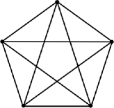
The cellular decomposition and its dual, in particular the surfaces and the dual links , constitute the structure needed for the smearing process.
Computation of holonomies
We have to compute holonomies of the left-invariant Ashtekar-Barbero connection , with
| (33) |
This task is easily accomplished if the path is a geodesic, as in our case.
Recall that the holonomy of the connection along the curve is the path-ordered exponential222The holonomy of the connection associated to a parametrized curve , , is the solution evaluated at of the matrix differential equation (34)
| (35) |
where the -th integral has the form
| (36) |
Here we have used an explicit parametrization of the geodesic in terms of the proper distance along the curve () and is the proper length of the curve. Now we exploit the fact that since are three left-invariant vector fields, and the spatial metric tensor is right-invariant333Of course, the spatial metric is both left and right-invariant. It is the unique bi-invariant metric tensor on , up to a global scale factor, which is fixed to be ., are Killing vectors Wald . It follows that the three scalars
| (37) |
are conserved quantities, i.e. constant along (spatial) geodesics. We can then easily compute the path-ordered exponential (35). Given
| (38) |
we have444Geodesics over that start at the identity element have the simple form , namely they are the 1-parameter subgroups of .
| (39) |
Notice that the first equality in (39) does not hold for any path connecting the initial and final points, but only for geodesic paths. In fact if it did work for general paths, since is path-independent, that would imply that the holonomy of the Ashtekar connection is path-independent, or equivalently, that the holonomy of any contractible loop is the identity (which means that the connection is flat). Instead, the Maurer-Cartan holonomy is given by formula (39) with , for any path.
Specifically, we are interested in holonomies along the oriented links of the embedded graph . A link goes from the source node to the target node of the geodesic link . In fact, as explained in Section II, we consider holonomies along half-links, from the source node to the point of intersection with the dual surface.
Take a node of and suppose all the four surrounding links are oriented as ‘outgoing’. It is clear that since the four links emanate from the node in isotropic directions, the four unit vectors defined in (37) are such that for . These can be thought as the unit vectors normal to the four faces of an equilateral tetrahedron in . For the general case, observe that unit vectors associated to different orientations of the path are related by . This fixes uniquely the full set of 10 unit vectors, up to a global rotation.
Moreover the length of a full link is
| (40) |
This can be easily seen considering the following geodesic on the unit Euclidean sphere :
| (43) |
Suppose we have chosen coordinates where this geodesic lies over one link of the graph. With the standard embedding555The standard embedding of in is (46) with real and . of in , it becomes clear that the two nodes , , viewed as vectors in , have scalar product . Now, since the previous geodesic (43), embedded in , has the form , imposing
| (47) |
we find the value for the geodesic length. To obtain the geodesic length for a sphere of different radius, we just multiply by the appropriate scale factor , so we prove (40).
Thus, we find that the holonomy of the Ashtekar-Barbero connection along half-link is
| (48) |
This completes the computation of holonomies. Notice that the dependence on in the holonomy is contained in the extrinsic curvature coefficient , that codes the embedding properties of the 3-sphere into the curved space-time.
Computation of fluxes
The computation of fluxes is more tricky as it relies on the definition (7). The flux depends on the surface as well as on the holonomies along a system of paths, as explained in section II. However, we shall not need those complicated details, as we are mostly interested in the unit-fluxes, and not in the explicit calculation of the modulus. In spite of this fact, the smearing process must not break the symmetries of the regular cellular decomposition we have chosen. In our case we can take a family of geodesics joining the intersection point with the generic point of integration on the surface. We have
| (49) |
where , , is the metric induced on the surface from , and is a unit vector given by
| (50) |
with
| (51) |
Let us explain our short notation. The rotation matrix is the holonomy in the adjoint representation of , that acts on the internal indices. It performs the parallel transport of the triad from the base point to the point of integration , along a geodesic path. Since we are averaging around the barycenter , we have clearly
| (52) |
where denotes the modulus of the flux, whose time dependence is easily recovered: . We denote the flux across the oriented surface punctured by the link . We have
| (53) |
It is important to remark that the unit fluxes in the last equation coincide with the unit directions that identify the 1-parameter subgroup of Ashtekar holonomies , namely with of equation (48). This is true because the orientations of the link and of the surface agree.
V FLRW: quantum state
We can now define the coherent spin-network for FLRW geometry as the one labeled by variables on links, as defined by the smearing process of previous section:
| (54) |
We now apply the decomposition (18) to obtain:
| (55) |
where is precisely the inverse of , namely there is no extra relative phase. As we anticipated in section II, the smearing process determines unambiguously the relative phase between ‘source’ and ‘target’ holonomies. In the asymptotic regime, this translates into a precise prescription for the relative phases of Livine-Speziale intertwiners, as we shall see in a moment.
The term proportional to in the exponent of (55) can be absorbed in the redefinition of the arbitrary phase of one of the , that is
| (56) |
in which
| (57) |
Notice that this choice of the relative phase between the ‘source’ and ‘target’ group elements is analogous to (actually, in the asymptotic regime coincide with) the canonical choice of relative phase for Livine-Speziale coherent intertwiners in the boundary of a flat 4-simplex of references Barrett et al. (2009, 2010). There, the canonical relative phase is obtained by the parallel transport of coherent states using the discrete spin-connection. Here instead the parallel transport is computed as the holonomy of the smooth spin-connection along geodesics of the 3-sphere.
The coherent spin-network with labels as in (54), or equivalently (56), can be written as a superposition over the ordinary spin-network orthonormal basis as
| (58) |
By the asymptotic formula (20), the asymptotic behavior of the coherent spin-network for large can be found. We find that for large scale factor , the FLRW coherent state is
| (59) |
with
| (60) | |||
| (61) | |||
| (62) |
and we have set the inverse heat-kernel times , to respect the symmetry of the regular cellular decomposition. Lastly, let us comment on the units in (60): by the definition (11), the dependence on the heat-kernel time in drops out, and we are left with the dimensionful factor . This is in agreement with the area spectrum of Loop Quantum Gravity. In the following we give specific examples.
Our construction applies to the case of flat space-time, provided that we consider the Riemannian signature and space-time topology . Indeed, in this case we are allowed to write the metric in polar coordinates in the form
| (63) |
where , as usual, is the metric tensor of a unit Euclidean 3-sphere. Thus (63) has the FLRW form, provided by the scale factor
| (64) |
and consistently with this latter relation the extrinsic curvature coefficient , defined by , is given by
| (65) |
The semiclassical state for Euclidean space-time is then characterized by the large scale behavior:
| (66) |
Remarkably, those coefficients are similar666A significant difference is that the heat-kernel coherent states discussed here present (asymptotically) a diagonal spin-spin correlation matrix, while a non-diagonal correlation matrix seems to be required from matching conditions in the graviton propagator calculation Bianchi et al. (2009). to those ones used in order to define correlation functions over flat space in the Spin Foam setting Rovelli (2006); Modesto and Rovelli (2005); Bianchi et al. (2006); Alesci and Rovelli (2007); Bianchi et al. (2009). In particular, the oscillatory factor which prescribes the extrinsic curvature matches exactly with the analogous phase factor originally advocated by Rovelli’s ansatz Rovelli (2006). More precisely, it matches with the one of reference Bianchi et al. (2009), which includes the correct dependence on the Immirzi parameter. Moreover, in the Spin Foam setting, the angle is interpreted as a -dimensional dihedral angle between two tetrahedra lying in the boundary of an equilateral, flat -simplex. Such a value of the dihedral angle is also responsible for the mechanism of coherent cancellation of phases, which yields the correct semiclassical behavior of the 2-point function.
In cosmology, de Sitter space-time is usually coordinatized in the form
| (67) |
so that the constant- surfaces are flat Euclidean spaces , and the scale factor grows exponentially in time. is the (constant) Hubble rate of expansion. We are not considering here such a kind of canonical surfaces. We rather consider a spherical slicing of de Sitter space-time attained by the use of the following coordinates:
| (68) |
in the Lorentzian case, and
| (69) |
in the Riemannian case. When de Sitter space-time is viewed as the homogeneous, isotropic solution of vacuum Einstein equations with cosmological constant , we have . This foliation of the de Sitter manifold corresponds, for the two space-time signatures, to
| (70) | |||
| (71) |
respectively.
As a final remark, notice that if we invert the sign of in (59), we obtain the the complex conjugate state, which is a different state, even though classically these two states correspond to the same solution of Einstein equations, but opposite space-time orientations. A different way to think about it is to consider parity transformations, enlarging to the full orthogonal group . Under a parity transformation, which is a large gauge transformation, the triad changes sign and the scalar coefficients transform as
| (72) | |||
| (73) |
so (59) and its complex conjugate are related by parity. This does not mean that Loop Quantum Gravity violates parity, as parity-related sectors in the kinematical Hilbert space could be super-selected by the dynamics Bojowald and Das (2008, 2008). Nevertheless, the issue of the parity behavior of Loop Quantum Gravity is tricky, as one of the fundamental variables, the Ashtekar-Barbero connection, does not transform simply. Moreover, the parity transformation requires to disentangle the extrinsic and intrinsic components from the connection, which is possible only by using the equations of motion.
Conclusions and outlook
We provided a class of coherent spin-network states for Loop Quantum Gravity which are peaked around FLRW-like geometries. The main result is the derivation of the semiclassical state for flat space-time used in Spin Foams from the canonical theory, and its generalization to curved (homogeneous and isotropic) backgrounds, for both Euclidean and Lorentzian signatures.
Our analysis gives further intuition on which aspects of classical General Relativity are captured by the truncation to a given graph of the phase space of Loop Quantum Gravity. We chose the complete 5-vertex graph (4-simplex graph), symmetrically embedded in the canonical hyper-surface, in order to compare the result with the standard boundary states of Spin Foam vertex amplitudes, but we stress that the construction can be easily generalized to different (e.g. very fine) graphs. The applications of such a class of coherent states in a context of cosmological interest could open new perspectives within the semiclassical analysis of the Spin Foam dynamics, as a possible development of a cosmological perturbation theory.
Taking into account a simple and highly symmetric semiclassical state is the natural way to perform a symmetric reduction within the full quantum theory, which can then be compared with the standard results of Loop Quantum Cosmology. We hope the simple coherent state discussed here (maybe the most simple) could shed light on this relationship. Finally, it would be interesting to investigate the relation (if any) of the de Sitter coherent state we presented in this paper with the Kodama ground state Kodama (1988); Smolin (2002); Freidel and Smolin (2004).
Acknowlegements
We thank Stephon Alexander and Carlo Rovelli for comments on the manuscript. This work was supported in part by the NSF grant PHY0854743, The George A. and Margaret M. Downsbrough Endowment and the Eberly research funds of Penn State. E.M. gratefully acknowledges support from “Fondazione Angelo della Riccia”. A.M. acknowledges support from NSF CAREER grant.
Appendix A Useful formulae
The Maurer-Cartan form in hyperspheric coordinates reads
| (74) | |||
| (75) | |||
| (76) |
with ranges .
References
- Ashtekar (1986) Abhay Ashtekar, “New Variables for Classical and Quantum Gravity,” Phys. Rev. Lett., 57, 2244–2247 (1986).
- Rovelli and Smolin (1990) Carlo Rovelli and Lee Smolin, “Loop Space Representation of Quantum General Relativity,” Nucl. Phys., B331, 80 (1990).
- Ashtekar and Isham (1992) Abhay Ashtekar and C. J. Isham, “Representations of the holonomy algebras of gravity and nonAbelian gauge theories,” Class. Quant. Grav., 9, 1433–1468 (1992), arXiv:hep-th/9202053 .
- (4) Carlo Rovelli, “Quantum gravity,” Cambridge, UK: Univ. Pr. (2004) 455 p.
- Thiemann (2001) Thomas Thiemann, “Modern canonical quantum general relativity,” (2001a), arXiv:gr-qc/0110034 .
- Bojowald (2003) Martin Bojowald, “Homogeneous loop quantum cosmology,” Class. Quant. Grav., 20, 2595–2615 (2003), arXiv:gr-qc/0303073 .
- Ashtekar et al. (2003) Abhay Ashtekar, Martin Bojowald, and Jerzy Lewandowski, “Mathematical structure of loop quantum cosmology,” Adv. Theor. Math. Phys., 7, 233–268 (2003), arXiv:gr-qc/0304074 .
- Bojowald (2001) Martin Bojowald, “Absence of singularity in loop quantum cosmology,” Phys. Rev. Lett., 86, 5227–5230 (2001), arXiv:gr-qc/0102069 .
- Bojowald (2002) Martin Bojowald, “Isotropic loop quantum cosmology,” Class. Quant. Grav., 19, 2717–2742 (2002), arXiv:gr-qc/0202077 .
- Ashtekar (2007) Abhay Ashtekar, “An Introduction to Loop Quantum Gravity Through Cosmology,” Nuovo Cim., B122, 135–155 (2007), arXiv:gr-qc/0702030 .
- Thiemann and Winkler (2001) T. Thiemann and O. Winkler, “Gauge field theory coherent states (GCS) III: Ehrenfest theorems,” Class. Quant. Grav., 18, 4629–4682 (2001a), arXiv:hep-th/0005234 .
- Bahr and Thiemann (2007) Benjamin Bahr and Thomas Thiemann, “Approximating the physical inner product of Loop Quantum Cosmology,” Class. Quant. Grav., 24, 2109–2138 (2007), arXiv:gr-qc/0607075 .
- Sahlmann and Thiemann (2006) Hanno Sahlmann and Thomas Thiemann, “Towards the QFT on curved spacetime limit of QGR. I: A general scheme,” Class. Quant. Grav., 23, 867–908 (2006a), arXiv:gr-qc/0207030 .
- Sahlmann and Thiemann (2006) Hanno Sahlmann and Thomas Thiemann, “Towards the QFT on curved spacetime limit of QGR. II: A concrete implementation,” Class. Quant. Grav., 23, 909–954 (2006b), arXiv:gr-qc/0207031 .
- Reisenberger and Rovelli (2000) Michael Reisenberger and Carlo Rovelli, “Spin foams as Feynman diagrams,” (2000), arXiv:gr-qc/0002083 .
- Perez (2003) Alejandro Perez, “Spin foam models for quantum gravity,” Class. Quant. Grav., 20, R43 (2003), arXiv:gr-qc/0301113 .
- Ashtekar et al. (2010) Abhay Ashtekar, Miguel Campiglia, and Adam Henderson, “Casting Loop Quantum Cosmology in the Spin Foam Paradigm,” Class. Quant. Grav., 27, 135020 (2010), arXiv:1001.5147 [gr-qc] .
- Livine and Speziale (2007) Etera R. Livine and Simone Speziale, “A new spinfoam vertex for quantum gravity,” Phys. Rev., D76, 084028 (2007), arXiv:0705.0674 [gr-qc] .
- Engle et al. (2008) Jonathan Engle, Etera Livine, Roberto Pereira, and Carlo Rovelli, “LQG vertex with finite Immirzi parameter,” Nucl. Phys., B799, 136–149 (2008), arXiv:0711.0146 [gr-qc] .
- Freidel and Krasnov (2008) Laurent Freidel and Kirill Krasnov, “A New Spin Foam Model for 4d Gravity,” Class. Quant. Grav., 25, 125018 (2008), arXiv:0708.1595 [gr-qc] .
- Magliaro et al. (2008) Elena Magliaro, Claudio Perini, and Carlo Rovelli, “Numerical indications on the semiclassical limit of the flipped vertex,” Class. Quant. Grav., 25, 095009 (2008), arXiv:0710.5034 [gr-qc] .
- Alesci et al. (2009) Emanuele Alesci, Eugenio Bianchi, Elena Magliaro, and Claudio Perini, “Intertwiner dynamics in the flipped vertex,” Class. Quant. Grav., 26, 185003 (2009), arXiv:0808.1971 [gr-qc] .
- Alesci et al. (2010) Emanuele Alesci, Eugenio Bianchi, Elena Magliaro, and Claudio Perini, “Asymptotics of LQG fusion coefficients,” Class. Quant. Grav., 27, 095016 (2010), arXiv:0809.3718 [gr-qc] .
- Conrady and Freidel (2008) Florian Conrady and Laurent Freidel, “On the semiclassical limit of 4d spin foam models,” Phys. Rev., D78, 104023 (2008), arXiv:0809.2280 [gr-qc] .
- Barrett et al. (2009) John W. Barrett, Richard J. Dowdall, Winston J. Fairbairn, Henrique Gomes, and Frank Hellmann, “Asymptotic analysis of the EPRL four-simplex amplitude,” J. Math. Phys., 50, 112504 (2009), arXiv:0902.1170 [gr-qc] .
- Barrett et al. (2010) John W. Barrett, Richard J. Dowdall, Winston J. Fairbairn, Frank Hellmann, and Roberto Pereira, “Lorentzian spin foam amplitudes: graphical calculus and asymptotics,” Class. Quant. Grav., 27, 165009 (2010), arXiv:0907.2440 [gr-qc] .
- Perini et al. (2009) Claudio Perini, Carlo Rovelli, and Simone Speziale, “Self-energy and vertex radiative corrections in LQG,” Phys. Lett., B682, 78–84 (2009), arXiv:0810.1714 [gr-qc] .
- Krajewski et al. (2010) Thomas Krajewski, Jacques Magnen, Vincent Rivasseau, Adrian Tanasa, and Patrizia Vitale, “Quantum Corrections in the Group Field Theory Formulation of the EPRL/FK Models,” (2010), arXiv:1007.3150 [gr-qc] .
- Geloun et al. (2010) Joseph Ben Geloun, Razvan Gurau, and Vincent Rivasseau, “EPRL/FK Group Field Theory,” (2010), arXiv:1008.0354 [hep-th] .
- Oeckl (2003) Robert Oeckl, “A ’general boundary’ formulation for quantum mechanics and quantum gravity,” Phys. Lett., B575, 318–324 (2003), arXiv:hep-th/0306025 .
- Rovelli (2006) Carlo Rovelli, “Graviton propagator from background-independent quantum gravity,” Phys. Rev. Lett., 97, 151301 (2006), arXiv:gr-qc/0508124 .
- Modesto and Rovelli (2005) Leonardo Modesto and Carlo Rovelli, “Particle scattering in loop quantum gravity,” Phys. Rev. Lett., 95, 191301 (2005), arXiv:gr-qc/0502036 .
- Bianchi et al. (2006) Eugenio Bianchi, Leonardo Modesto, Carlo Rovelli, and Simone Speziale, “Graviton propagator in loop quantum gravity,” Class. Quant. Grav., 23, 6989–7028 (2006), arXiv:gr-qc/0604044 .
- Alesci and Rovelli (2007) Emanuele Alesci and Carlo Rovelli, “The complete LQG propagator: I. Difficulties with the Barrett-Crane vertex,” Phys. Rev., D76, 104012 (2007), arXiv:0708.0883 [gr-qc] .
- Bianchi et al. (2009) Eugenio Bianchi, Elena Magliaro, and Claudio Perini, “LQG propagator from the new spin foams,” Nucl. Phys., B822, 245–269 (2009), arXiv:0905.4082 [gr-qc] .
- Rovelli and Vidotto (2008) Carlo Rovelli and Francesca Vidotto, “Stepping out of Homogeneity in Loop Quantum Cosmology,” Class. Quant. Grav., 25, 225024 (2008), arXiv:0805.4585 [gr-qc] .
- Battisti et al. (2010) Marco Valerio Battisti, Antonino Marcianò, and Carlo Rovelli, “Triangulated Loop Quantum Cosmology: Bianchi IX and inhomogenous perturbations,” Phys. Rev., D81, 064019 (2010), arXiv:0911.2653 [gr-qc] .
- Marcianò (2010) Antonino Marcianò, “Towards inhomogeneous loop quantum cosmology: triangulating Bianchi IX with perturbations,” (2010), arXiv:1003.0352 [gr-qc] .
- Battisti and Marcianò (2010) Marco Valerio Battisti and Antonino Marcianò, “Big Bounce in Dipole Cosmology,” (2010), arXiv:1010.1258 [gr-qc] .
- Bianchi et al. (2010) Eugenio Bianchi, Carlo Rovelli, and Francesca Vidotto, “Towards Spinfoam Cosmology,” Phys. Rev., D82, 084035 (2010a), arXiv:1003.3483 [gr-qc] .
- Rovelli (2010) Carlo Rovelli, “A new look at loop quantum gravity,” (2010), arXiv:1004.1780 [gr-qc] .
- Bianchi et al. (2010) Eugenio Bianchi, Elena Magliaro, and Claudio Perini, “Coherent spin-networks,” Phys. Rev., D82, 024012 (2010b), arXiv:0912.4054 [gr-qc] .
- Dasgupta (2003) Arundhati Dasgupta, “Coherent states for black holes,” JCAP, 0308, 004 (2003), arXiv:hep-th/0305131 .
- Freidel and Speziale (2010) Laurent Freidel and Simone Speziale, “Twisted geometries: A geometric parametrisation of SU(2) phase space,” Phys. Rev., D82, 084040 (2010a), arXiv:1001.2748 [gr-qc] .
- Rovelli and Speziale (2010) Carlo Rovelli and Simone Speziale, “On the geometry of loop quantum gravity on a graph,” Phys. Rev., D82, 044018 (2010), arXiv:1005.2927 [gr-qc] .
- Freidel and Speziale (2010) Laurent Freidel and Simone Speziale, “From twistors to twisted geometries,” Phys. Rev., D82, 084041 (2010b), arXiv:1006.0199 [gr-qc] .
- Thiemann (2001) T. Thiemann, “Quantum spin dynamics (QSD). VII: Symplectic structures and continuum lattice formulations of gauge field theories,” Class. Quant. Grav., 18, 3293–3338 (2001b), arXiv:hep-th/0005232 .
- Hall (1994) Brian C. Hall, “The Segal-Bargmann Coherent State Transform for Compact Lie Groups,” J. Funct. Anal., 122, 103–151 (1994).
- Hall (2002) Brian C. Hall, “Geometric quantization and the generalized Segal-Bargmann transform for Lie groups of compact type,” Comm. Math. Phys., 226, 233–268 (2002).
- Ashtekar et al. (1996) Abhay Ashtekar, Jerzy Lewandowski, Donald Marolf, Jose Mourao, and Thomas Thiemann, “Coherent state transforms for spaces of connections,” J. Funct. Anal., 135, 519–551 (1996), arXiv:gr-qc/9412014 .
- Thiemann (2001) Thomas Thiemann, “Gauge field theory coherent states (GCS). I: General properties,” Class. Quant. Grav., 18, 2025–2064 (2001c), arXiv:hep-th/0005233 .
- Thiemann and Winkler (2001) T. Thiemann and O. Winkler, “Gauge field theory coherent states (GCS). II: Peakedness properties,” Class. Quant. Grav., 18, 2561–2636 (2001b), arXiv:hep-th/0005237 .
- Bahr and Thiemann (2009) Benjamin Bahr and Thomas Thiemann, “Gauge-invariant coherent states for Loop Quantum Gravity II: Non-abelian gauge groups,” Class. Quant. Grav., 26, 045012 (2009), arXiv:0709.4636 [gr-qc] .
- Bianchi et al. (2010) Eugenio Bianchi, Elena Magliaro, and Claudio Perini, “Spinfoams in the holomorphic representation,” (2010c), arXiv:1004.4550 [gr-qc] .
- (55) Robert M. Wald, “General Relativity,” Chicago, Usa: Univ. Pr. ( 1984) 491p.
- Bojowald and Das (2008) Martin Bojowald and Rupam Das, “Canonical Gravity with Fermions,” Phys. Rev., D78, 064009 (2008a), arXiv:0710.5722 [gr-qc] .
- Bojowald and Das (2008) Martin Bojowald and Rupam Das, “Fermions in Loop Quantum Cosmology and the Role of Parity,” Class. Quant. Grav., 25, 195006 (2008b), arXiv:0806.2821 [gr-qc] .
- Kodama (1988) Hideo Kodama, “Specialization of ashtekar’s formalism to bianchi cosmology,” Progress of Theoretical Physics, 80, 1024–1040 (1988).
- Smolin (2002) Lee Smolin, “Quantum gravity with a positive cosmological constant,” (2002), arXiv:hep-th/0209079 .
- Freidel and Smolin (2004) Laurent Freidel and Lee Smolin, “The linearization of the Kodama state,” Class. Quant. Grav., 21, 3831–3844 (2004), arXiv:hep-th/0310224 .