HyperANF: Approximating the Neighbourhood Function of Very Large Graphs on a Budget

Abstract

The neighbourhood function $N_{G}(t)$ of a graph $G$ gives, for each $t\in\mathbf{N}$, the number of pairs of nodes $\langle x,y\rangle$ such that $y$ is reachable from $x$ in less that $t$ hops. The neighbourhood function provides a wealth of information about the graph [PGF02] (e.g., it easily allows one to compute its diameter), but it is very expensive to compute it exactly. Recently, the ANF algorithm [PGF02] (approximate neighbourhood function) has been proposed with the purpose of approximating $N_{G}(t)$ on large graphs. We describe a breakthrough improvement over ANF in terms of speed and scalability. Our algorithm, called HyperANF, uses the new HyperLogLog counters [FFGM07] and combines them efficiently through broadword programming [Knu07]; our implementation uses task decomposition to exploit multi-core parallelism. With HyperANF, for the first time we can compute in a few hours the neighbourhood function of graphs with billions of nodes with a small error and good confidence using a standard workstation.

Then, we turn to the study of the distribution of distances between reachable nodes (that can be efficiently approximated by means of HyperANF), and discover the surprising fact that its index of dispersion provides a clear-cut characterisation of proper social networks vs. web graphs. We thus propose the spid (Shortest-Paths Index of Dispersion) of a graph as a new, informative statistics that is able to discriminate between the above two types of graphs. We believe this is the first proposal of a significant new non-local structural index for complex networks whose computation is highly scalable.

1 Introduction

The neighbourhood function $N_{G}(t)$ of a graph returns for each $t\in\mathbf{N}$ the number of pairs of nodes $\langle x,y\rangle$ such that $y$ is reachable from $x$ in less that $t$ steps. It provides data about how fast the “average ball” around each node expands. From the neighbourhood function, several interesting features of a graph can be estimated, and in this paper we are in particular interested in the effective diameter, a measure of the “typical” distance between nodes.

Palmer, Gibbons and Faloutsos [PGF02] proposed an algorithm to approximate the neighbourhood function (see their paper for a review of previous attempts at approximate evaluation); the authors distribute an associated tool, snap, which can approximate the neighbourhood function of medium-sized graphs. The algorithm keeps track of the number of nodes reachable from each node using Flajolet–Martin counters, a kind of sketch that makes it possible to compute the number of distinct elements of a stream in very little space. A key observation was that counters associated to different streams can be quickly combined into a single counter associated to the concatenation of the original streams.

In this paper, we describe HyperANF—a breakthrough improvement over ANF in terms of speed and scalability. HyperANF uses the new HyperLogLog counters [FFGM07], and combines them efficiently by means of broadword programming [Knu07]. Each counter is made by a number of registers, and the number of registers depends only on the required precision. The size of each register is doubly logarithmic in the number of nodes of the graph, so HyperANF, for a fixed precision, scales almost linearly in memory (i.e., $O(n\log\log n)$). By contrast, ANF memory requirement is $O(n\log n)$.

Using HyperANF, for the first time we can compute in a few hours the neighbourhood function of graphs with more than one billion nodes with a small error and good confidence using a standard workstation with 128 GB of RAM. Our algorithms are implement in a tool distributed as free software within the WebGraph framework.

Armed with our tool, we study several datasets, spanning from small social networks to very large web graphs. We isolate a statistically defined feature, the index of dispersion of the distance distribution, and show that it is able to tell “proper” social networks from web graphs in a natural way.

2 Related work

HyperANF is an evolution of ANF [PGF02], which is implemented by the tool snap. We will give some timing comparison with snap, but we can only do it for relatively small networks, as the large memory footprint of snap precludes application to large graphs.

Recently, a MapReduce-based distributed implementation of ANF called HADI [KTA⁺10] has been presented. HADI runs on one of the fifty largest supercomputers—the Hadoop cluster M45. The only published data about HADI’s performance is the computation of the neighbourhood function of a Kronecker graph with 2 billion links, which required half an hour using 90 machines. HyperANF can compute the same function in less than fifteen minutes on a laptop.

The rather complete survey of related literature in [KTA⁺10] shows that essentially no data mining tool was able before ANF to approximate the neighbourhood function of very large graphs reliably. A remarkable exception is Cohen’s work [Coh97], which provides strong theoretical guarantees but experimentally turns out to be not as scalable as the ANF approach; it is worth noting, though, that one of the proposed applications of [Coh97] (On-line estimation of weights of growing sets) is structurally identical to ANF.

All other results published before ANF relied on a small number of breadth-first visits on uniformly sampled nodes—a process that has no provable statistical accuracy or precision. Thus, in the rest of the paper we will compare experimental data with snap and with the published data about HADI.

3 HyperANF

In this section, we present the HyperANF algorithm for computing an approximation of the neighbourhood function of a graph; we start by recalling from [FFGM07] the notion of HyperLogLog counter upon which our algorithm relies. We then describe the algorithm, discuss how it can be implemented to be run quickly using broadword programming and task decomposition, and give results about its memory requirements and precision.

3.1 HyperLogLog counters

HyperLogLog counters, as described in [FFGM07] (which is based on [DF03]), are used to count approximately the number of distinct elements in a stream. For the purposes of the present paper, we need to recall briefly their behaviour. Essentially, these probabilistic counters are a sort of approximate set representation to which, however, we are only allowed to pose questions about the (approximate) size of the set.

Let $\mathscr{D}$ be a fixed domain and $h:\mathscr{D}\to 2^{\infty}$ be a hash function mapping each element of $\mathscr{D}$ into an infinite binary sequence. The function is fixed with the only assumption that “bits of hashed values are assumed to be independent and to have each probability $\frac{1}{2}$ of occurring” [FFGM07].

For a given $x\in 2^{\infty}$, let $h_{t}(x)$ denote the sequence made by the leftmost $t$ bits of $h(x)$, and $h^{t}(x)$ be the sequence of remaining bits of $x$; $h_{t}$ is identified with its corresponding integer value in the range $\{\,0,1,\dots,2^{t}-1\,\}$. Moreover, given a binary sequence $w$, we let $\rho^{+}(w)$ be the number of leading zeroes in $w$ plus one (e.g., $\rho^{+}(00101)=3$). Unless otherwise specified, all logarithms are in base 2.

0	$h:\mathscr{D}\to 2^{\infty}$, a hash function from the domain of items
1	$M[-]$ the counter, an array of $m=2^{b}$ registers
2		(indexed from 0) and set to $-\infty$
3
4	function $\mathrm{add}(\text{$M$: counter},\text{$x$: item})$
5	begin
6		$i\leftarrow h_{b}(x)$;
7		$M[i]\leftarrow\max\bigl{\{}M[i],\rho^{+}\bigl{(}h^{b}(x)\bigr{)}\bigr{\}}$
8	end; // function add
9
10	function $\mathrm{size}(\text{$M$: counter})$
11	begin
12		$Z\leftarrow\left(\sum_{j=0}^{m-1}2^{-M[j]}\right)^{-1}$;
13		return $E=\alpha_{m}m^{2}Z$
14	end; // function size
15
16	foreach item $x$ seen in the stream begin
17		add($M$,$x$)
18	end;
19	print $\mathrm{size}(M)$

Algorithm 1 The Hyperloglog counter as described in [FFGM07]: it allows one to count (approximately) the number of distinct elements in a stream. $\alpha_{m}$ is a constant whose value depends on $m$ and is provided in [FFGM07]. Some technical details have been simplified.

The value $E$ printed by Algorithm 1 is [FFGM07][Theorem 1] an asymptotically almost unbiased estimator for the number $n$ of distinct elements in the stream; for $n\to\infty$, the relative standard deviation (that is, the ratio between the standard deviation of $E$ and $n$) is at most $\beta_{m}/\sqrt{m}\leq 1.06/\sqrt{m}$, where $\beta_{m}$ is a suitable constant (given in [FFGM07]). Moreover [DF03] even if the size of the registers (and of the hash function) used by the algorithm is unbounded, one can limit it to $\log\log(n/m)+\omega(n)$ bits obtaining almost certainly the same output ($\omega(n)$ is a function going to infinity arbitrarily slowly); overall, the algorithm requires $(1+o(1))\cdot m\log\log(n/m)$ bits of space (this is the reason why these counters are called HyperLogLog). Here and in the rest of the paper we tacitly assume that $m\geq 64$ and that registers are made of $\lceil\log\log n\rceil$ bits.

3.2 The HyperANF algorithm

The approximate neighbourhood function algorithm described in [PGF02] is based on the observation that $B(x,r)$, the ball of radius $r$ around node $x$, satisfies

$$B(x,r)=\bigcup_{x\to y}B(y,r-1).$$

Since $B(x,0)=\{\,x\,\}$, we can compute each $B(x,r)$ incrementally using sequential scans of the graph (i.e., scans in which we go in turn through the successor list of each node). The obvious problem is that during the scan we need to access randomly the sets $B(x,r-1)$ (the sets $B(x,r)$ can be just saved on disk on a update file and reloaded later). Here probabilistic counters come into play; to be able to use them, though, we need to endow counters with a primitive for the union. Union can be implemented provided that the counter associated to the stream of data $AB$ can be computed from the counters associated to $A$ and $B$; in the case of HyperLogLog counters, this is easily seen to correspond to maximising the two counters, register by register.

The observations above result in Algorithm 2: the algorithm keeps one HyperLogLog counter for each node; at the $t$-th iteration of the main loop, the counter $c[v]$ is in the same state as if it would have been fed with $B(v,t)$, and so its expected value is $|B(v,t)|$. As a result, the sum of all $c[v]$’s is an (almost) unbiased estimator of $N_{G}(t)$ (for a precise statement, see Theorem 1).

0	$c[-]$, an array of $n$ HyperLogLog counters
1
2	function $\mathrm{union}(\text{$M$: counter},\text{$N$: counter})$
3		foreach $i<m$ begin
4			$M[i]\leftarrow\max(M[i],N[i])$
5		end
6	end; // function union
7
8	foreach $v\in n$ begin
9		add $v$ to $c[v]$
10	end;
11	$t\leftarrow 0$;
12	do begin
13		$s\leftarrow\sum_{v}\mathrm{size}(c[v])$;
14		Print $s$ (the neighbourhood function $N_{G}(t)$)
15		foreach $v\in n$ begin
16			$m\leftarrow c[v]$;
17			foreach $v\rightarrow w$ begin
18				$m\leftarrow\mathrm{union}(c[w],m)$
19			end;
20			write $\langle v,m\rangle$ to disk
21		end;
22		Read the pairs $\langle v,m\rangle$ and update the array $c[-]$
23		$t\leftarrow t+1$
24	until no counter changes its value.

Algorithm 2 The basic HyperANF algorithm in pseudocode. The algorithm uses, for each node $i\in n$, an initially empty HyperLogLog counter $c_{i}$. The function $\mathrm{union}(-,-)$ maximises two counters register by register.

We remark that the only sound way of running HyperANF (or ANF) is to wait for all counters to stabilise (e.g., the last iteration must leave all counters unchanged). As we will see, any alternative termination condition may lead to arbitrarily large mistakes on pathological graphs.

3.3 HyperANF at hyper speed

Up to now, HyperANF has been described just as ANF with HyperLogLog counters. The effect of this change is an exponential reduction in the memory footprint and, consequently, in memory access time. We now describe the the algorithmic and engineering ideas that made HyperANF much faster, actually so fast that it is possible to run it up to stabilisation.

Union via broadword programming. Given two HyperLogLog counters that have been set by streams $A$ and $B$, the counter associated to the stream $AB$ can be build by maximising in parallel the registers of each counter. That is, the register $i$ of the new counter is given by the maximum between the $i$-th register of the first counter and the $i$-th register of the second counter.

Each time we scan a successor list, we need to maximise a large number of registers and store the resulting counter. The immediate way of obtaining this result requires extracting the value of each register, maximise it with the other corresponding registers, and writing down the result in a temporary counter. This process is extremely slow, as registers are packed in 64-bit memory words. In the case of Flajolet–Martin counters, the problem is easily solved by computing the logical OR of the words containing the registers. In our case, we resort to broadword programming techniques. If the machine word is $w$, we assume that at least $w$ registers are allocated to each counter, so each set of registers is word-aligned.

Let $\mathbin{\gg}$ and $\mathbin{\ll}$ denote right and left (zero-filled) shifting, $\mathbin{\&}$, $\mathbin{|}$ and $\oplus$ denote bit-by-bit not, and, or, and xor; $\overline{x}$ denotes the bit-by-bit complement of $x$.

We use $L_{k}$ to denote the constant whose ones are in position $0$, $k$, $2k$, …  that is, the constant with the lowest bit of each $k$-bit subword set (e.g, $L_{8}=0x01010101010101010101$). We use $H_{k}$ to denote $L_{k}\mathbin{\ll}k-1$, that is, the constant with the highest bit of each $k$-bit subword set (e.g, $H_{8}=0x8080808080808080$).

It is known (see [Knu07], or [Vig08] for an elementary proof), that the following expression

$$x<_{k}^{u}y:=\Bigl{(}\bigl{(}\,((x\mathbin{|}H_{k})-(y\mathbin{\&}\overline{H_{k}}))\mathbin{|}{x\oplus y}\bigr{)}\oplus(x\mathbin{|}\overline{y})\Bigr{)}\mathbin{\&}H_{k}.$$

performs a parallel unsigned comparison $k$-by-$k$-bit-wise. At the end of the computation, the highest bit of each block of $k$ bits will be set iff the corresponding comparison is true (i.e., the value of the block in $x$ is strictly smaller than the value of the block in $y$).

Once we have computed $x<_{k}^{u}$, we generate a mask that is made entirely of 1s, or of 0s, for each $k$-bit block, depending on whether we should select the value of $x$ or $y$ for that block:

$$m=\biggl{(}\Bigl{(}\bigl{(}(x<_{k}^{u}y)\mathbin{\gg}k-1\mathbin{|}H_{k}\bigr{)}-L_{k}\Bigr{)}\mathbin{|}H_{k}\biggr{)}\oplus(x<_{k}^{u}y)$$

This formula works by moving the high bit denoting the result of the comparison to the least significant bit (of each $k$-bit block). Then, we or with $H_{k}$ and subtract $1$ from each block, obtaining either a mask with just the high bit set (if we were starting from 1) or a mask with all bits sets except for the high bit (if we were starting from 0). The last two operation fix those values so that they become $00\cdots 0$ or $11\cdots 1$. The result of the maximisation process is now just $x\mathbin{\&}m\mathbin{|}y\mathbin{\&}\overline{m}$.

This discussion assumed that the set of registers of a counter is stored in a single machine word. In a realistic setting, the registers are spread among several consecutive words, and we use multiple precision subtractions and shifts to apply the expressions above on a sequence of words. All other (logical) operations have just to be applied to each word in sequence.

All in all, by using the techniques above we can improve the speed of maximisation by a factor of $w/k$, which in our case is about 13 (for graphs of up to $2^{32}$ nodes). This actually results in a sixfold speed improvement of the overall application in typical cases (e.g., web graphs and $b=8$), as about 90% of the computation time is spent in maximisation.

Parallelisation via task decomposition. Although HyperANF is written as a sequential algorithm, the outer loop lends itself to be executed in parallel, which can be extremely fruitful on a modern multicore architecture; in particular, we approach this idea using task decomposition. We divide the iteration on the whole set of nodes into a set of small tasks (in the order of the thousands), where each task consists in iterating on a contiguous segment of nodes. A pool of threads picks up the first available task and solves it: as a result, we obtain a performance improvement that is linear in the number of cores. Threads can be designed to be extremely agile, helped by WebGraph’s facilities which allow us to provide each thread with a lightweight copy of the graph that shares the bitstream and associated information with all other threads.

Tracking modified counters. It is an easy observation that a counter $c$ that does not change its value is not useful for the next step of the computation: all counters using $c$ during their update would not change their value when maximising with $c$ (and we do not even need to write $c$ on disk). We thus keep track of modified counters and skip altogether the maximisation step with unmodified ones. Since, as we already remarked, 90% of computation time is spent in maximisation, this approach leads to a large speedup after the first phases of the computation, when most counters are stabilised.

For the same reason, we keep track of the harmonic partial sums of small blocks (e.g., $64$) of counters. The amount of memory required is negligible, but if no counter in the block has been modified, we can avoid a costly computation.

Systolic computation. HyperANF can be run in systolic mode. In this case, we use also the transposed graph: whenever a counter changes, it signals back to its predecessors that at the next round they could change their values. Now, at each iteration nodes that have not been signalled are entirely skipped during the computation. Systolic computations are fundamental to get high-precision runs, as they reduce the cost of an iteration to scanning only the arcs of the graph that are actually moving information around. We switch to systolic computation when less than one quarter of the counters change their values.

3.4 Correctness, errors and memory usage

Very little has been published about the statistical behaviour of ANF. The statistical properties of approximate counters are well known, but the values of such counters for each node are highly dependent, and adding them in a large amount can in principle lead to an arbitrarily large variance. Thus, making precise statistical statements about the outcome of a computation of ANF or HyperANF requires some care. The discussion in the following sections is based on HyperANF, but its results can be applied mutatis mutandis to ANF as well.

Consider the output $\hat{N}_{G}(t)$ of algorithm 2 at a fixed iteration $t$. We can see it as a random variable

$$\hat{N}_{G}(t)=\sum_{i\in n}X_{i,t}$$

where each $X_{i,t}$ is the HyperLogLog counter that counts nodes reached by node $i$ in $t$ steps; what we want to prove in this section is a bound on the relative standard deviation of $\hat{N}_{G}(t)$ (such a proof, albeit not difficult, is not provided in the papers about ANF). First observe that [FFGM07], for a fixed a number of registers $m$ per counter, the standard deviation of $X_{i,t}$ satisfies

$$\frac{\sqrt{\mathrm{Var}[X_{i,t}]}}{|B(i,t)|}\leq\eta_{m},$$

where $\eta_{m}$ is the guaranteed relative standard deviation of a HyperLogLog counter. Using the subadditivity of standard deviation (i.e., if $A$ and $B$ have finite variance, $\sqrt{\mathrm{Var}[A+B]}\leq\sqrt{\mathrm{Var}[A]}+\sqrt{\mathrm{Var}[B]}$), we prove the following

Theorem 1

The output $\hat{N}_{G}(t)$ of Algorithm 2 at the $t$-th iteration is an asymptotically almost unbiased estimator of $N_{G}(t)$, that is

$$\frac{E[\hat{N}_{G}(t)]}{N_{G}(t)}=1+\delta_{1}(n)+o(1)\text{ for $n\to\infty$},$$

where $\delta_{1}$ is the same as in [FFGM07][Theorem 1] (and $|\delta_{1}(x)|<5\cdot 10^{-5}$ as soon as $m\geq 16$).

Moreover, $\hat{N}_{G}(t)$ has the same relative standard deviation of the $X_{i}$’s, that is

$$\frac{\sqrt{\mathrm{Var}[\hat{N}_{G}(t)]}}{N_{G}(t)}\leq\eta_{m}.$$

Proof. We have that $E[\hat{N}_{G}(t)]=E\bigl{[}\sum_{i\in n}X_{i,t}\bigr{]}$. By Theorem 1 of [FFGM07], $E[X_{i,t}]=|B(i,t)|\left(1+\delta_{1}(n)+o(1)\right)$, hence the first statement. For the second result, we have:

$$\frac{\sqrt{\mathrm{Var}[\hat{N}_{G}(t)]}}{N_{G}(t)}\leq\frac{\sum_{i\in n}\sqrt{\mathrm{Var}[X_{i}]}}{N_{G}(t)}\leq\frac{\eta_{m}\sum_{i\in n}|B(i,t)|}{N_{G}(t)}=\eta_{m}.$$

 

Since, as we recalled in Section 3.1, the relative standard deviation $\eta_{m}$ satisfies $\eta_{m}\leq 1.06/\sqrt{m}$, to get a specific value $\eta$ it is sufficient to choose $m\approx 1.12/\eta^{2}$; this assumption yields an overall space requirement of about

$$\frac{1.12}{\eta^{2}}n\log\log n\qquad\text{bits}$$

(here, we used the obvious upper bound $|B(i,t)|\leq n$). For instance, to obtain a relative standard deviation of $9.37\%$ (in every iteration) on a graph of one billion nodes one needs $74.5$ GB of main memory for the registers (for a comparison, snap would require $550$ GB). Note that since we write to disk the new values of the registers, this is actually the only significant memory requirement (the graph can be kept on disk and mapped in memory, as it is scanned almost sequentially).

Applying Chebyshev’s inequality, we obtain the following:

Corollary 1

For every $\varepsilon$,

$$\Pr\left[\frac{\hat{N}_{G}(t)}{N_{G}(t)}\in(1-\varepsilon,1+\varepsilon)\right]\geq 1-\frac{\eta_{m}^{2}}{\varepsilon^{2}}.$$

In [FFGM07] it is argued that the HyperLogLog error is approximately Gaussian; the counters, however, are not statistically independent and in fact the overall error does not appear to be normally distributed. Nonetheless, for every fixed $t$, the random variable $\hat{N}_{G}(t)$ seems to be unimodal (for example, the average p-value of the Dip unimodality test [HH85] for the cnr-2000 dataset is $0.011$), so we can apply the Vysochanskiĭ-Petunin inequality [VP82], obtaining the bound

$$\Pr\left[\frac{\hat{N}_{G}(t)}{N_{G}(t)}\in(1-\varepsilon,1+\varepsilon)\right]\geq 1-\frac{4\eta_{m}^{2}}{9\varepsilon^{2}}.$$

In the rest of the paper, to state clearly our theorems we will always assume error $\varepsilon$ with confidence $1-\delta$. It is useful, as a practical reminder, to note that because of the above inequality for each point of the neighbourhood function we can assume a relative error of $k\eta_{m}$ with confidence $1-4/(9k^{2})$ (e.g., $2\eta_{m}$ with $90$% confidence, or $3\eta_{m}$ with $95$% confidence).

As an empirical counterpart to the previous results, we considered a relatively small graph of about $325\,000$ nodes (cnr-2000, see Section 6 for a full description) for which we can compute the exact neighbourhood function $N_{G}(-)$; we ran HyperANF 500 times with $m=256$. At least $96$% of the samples (for all $t$) has a relative error smaller than twice the theoretical relative standard deviation $6.62\%$. The percentage jumps up to $100$% for three times the relative standard deviation, showing that the distribution of the values behaves better than what the theory would guarantee.

4 Deriving useful data

As advocated in [PGF02], being able to estimate the neighbourhood function on real-world networks has several interesting applications. Unfortunately, all published results we are aware of lack statistical satellite data (such as confidence intervals, or distribution of the computed values) that make it possible to compare results from different research groups. Thus, in this section we try to discuss in detail how to derive useful data from an approximation of the neighbourhood function.

The distance cdf. We start from the apparently easy task of computing the cumulative distribution function of distances of the graph $G$ (in short, distance cdf), which is the function $H_{G}(t)$ that gives the fraction of reachable pairs at distance at most $t$, that is,

$$H_{G}(t)=\frac{N_{G}(t)}{\max_{t}N_{G}(t)}.$$

In other words, given an exact computation of the neighbourhood function, the distance cdf can be easily obtained by dividing all values by the largest one. Being able to estimate $N_{G}(t)$ allows one to produce a reliable approximation of the distance cdf:

Theorem 2

Assume $N_{G}(t)$ is known for each $t$ with error $\varepsilon$ and confidence $1-\delta$, that is

$$\Pr\left[\frac{\hat{N}_{G}(t)}{N_{G}(t)}\in(1-\varepsilon,1+\varepsilon)\right]\geq 1-\delta.$$

Let $\hat{H}_{G}(t)=\hat{N}_{G}(t)/\max_{t}\hat{N}_{G}(t)$. Then $\hat{H}_{G}(t)$ is an (almost) unbiased estimator for $H_{G}(t)$; moreover, for a fixed sequence ${t}_{0}$, ${t}_{1}$, $\dots\,$, ${t}_{k-1}$, for every $\varepsilon$ and all $0\leq i<k$ we have that $\hat{H}_{G}(t_{k})$ is known with error $2\varepsilon$ and confidence $1-(k+1)\delta$, that is,

$$\Pr\left[\bigwedge_{i\in k}\frac{\hat{H}_{G}(t_{i})}{H_{G}(t_{i})}\in(1-2\varepsilon,1+2\varepsilon)\right]\geq 1-(k+1)\delta.$$

Proof. Note that if

$$1-\varepsilon\leq\hat{N}_{G}(t)/N_{G}(t)\leq 1+\varepsilon$$

holds for every $t$, then a fortiori

$$1-\varepsilon\leq\max_{t}\hat{N}_{G}(t)/\max_{t}N_{G}(t)\leq 1+\varepsilon$$

(because, although the maxima might be first attained at different values of $t$, the same holds for any larger values). As a consequence,

$$1-2\varepsilon\leq\frac{1-\varepsilon}{1+\varepsilon}\leq\frac{\hat{H}_{G}(t)}{H_{G}(t)}\leq\frac{1+\varepsilon}{1-\varepsilon}\leq 1+2\varepsilon.$$

The probability $1-(k+1)\delta$ is immediate from the union bound, as we are considering $k+1$ events at the same time.  

Note two significant limitations: first of all, making precise statements (i.e., with confidence) about all points of $H_{G}(t)$ requires a very high initial error and confidence. Second, the theorem holds if HyperANF has been run up to stabilisation, so that the probabilistic guarantees of HyperLogLog hold for all $t$.

The first limitation makes in practice impossible to get directly sensible confidence intervals, for instance, for the average distance or higher moments of the distribution (we will elaborate further on this point later). Thus, only statements about a small, finite number of points can be approached directly.

The second limitation is somewhat more serious in theory, albeit in practice it can be circumvented making suitable assumptions about the graph under examination (which however should be clearly stated along the data). Consider the graph $G$ made by two $k$-cliques joined by a unidirectional path of $\ell$ nodes (see Figure 2). Even neglecting the effect of approximation, $G$ can “fool” HyperANF (or ANF) so that the distance cdf is completely wrong (see Figure 1) when using any stopping criterion that is not stabilisation.

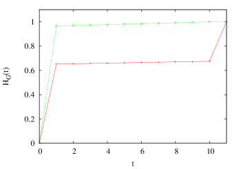
Figure 1: The real cdf of the graph in Figure 2 (+), and the one that would be computed using any termination condition that is not stabilisation (*); here $\ell=10$ and $k=260$.

Figure 2: Two $k$-cliques joined by a unidirectional path of $\ell$ nodes: terminating even one step earlier than stabilisation completely miscalculates the distance cdf (see Figure 1); the effective diameter is $\ell+1$, but terminating even just one step earlier than stabilisation yields an estimated effective diameter of 1.

Indeed, the exact neighbourhood function of $G$ is given by:

$$N_{G}(t)=\begin{cases}2k+\ell\qquad\text{if $t=0$}\\ (t+1)\left(2k+\ell-\frac{t}{2}\right)-2k+2k^{2}&\text{if $1\leq t\leq\ell$}\\ (\ell+1)\left(2k+\frac{\ell}{2}\right)-2k+3k^{2}&\text{if $\ell<t$.}\end{cases}$$

The key observation is that the very last value is significantly larger than all previous values, as at the last step the nodes of the right clique become reachable from the nodes of the first clique. Thus, if iteration stops before stabilisation, the normalisation factor used to compute the cdf will be smaller by $\approx k^{2}$ than the actual value, causing a completely wrong estimation of the cdf, as shown in Figure 1.

Although this counterexample (which can be easily adapted to be symmetric) is definitely pathological, it suggests that a particular care should be taken when handling graphs that present narrow “tubes” connecting large connected components: in such scenarios, the function $N_{G}(t)$ exhibits relatively long plateaux (preceded and followed by sharp bumps) that may fool the computation of the cdf.

The effective diameter. The first application of ANF was the computation of the effective diameter. The effective diameter of $G$ at $\alpha$ is the smallest $t_{0}$ such that $H_{G}(t_{0})\geq\alpha$; when $\alpha$ is omitted, it is assumed to be $\alpha=.9$. The interpolated effective diameter is obtained in the same way on the linear interpolation of the points of the neighbourhood function.

Since that the function $\hat{H}_{G}(t)$ is necessarily monotone in $t$ (independently of the approximation error), from Theorem 2 we obtain:

Corollary 2

Assume $\hat{N}_{G}(t)$ is known for each $t$ with error $\varepsilon$ and confidence $1-\delta$, and there are points $s$ and $t$ such that

$$\frac{\hat{H}_{G}(s)}{1-2\varepsilon}\leq\alpha\leq\frac{\hat{H}_{G}(t)}{1+2\varepsilon}.$$

Then, with probability $1-3\delta$ the effective diameter at $\alpha$ lies in $[s\,\mathpunct{\ldotp\ldotp}t]$.

Unfortunately, since the effective diameter depends sensitively on the distance cdf, again termination conditions can produce arbitrary errors. Getting back to the example of Figure 2, with a sufficiently large $k$, for example $k=2\ell^{2}+5\ell+2$, the effective diameter is $\ell+1$, which would be correctly output after $\ell+1$ iterations, whereas even stopping one step earlier (i.e., with $t=\ell$) would produce $1$ as output, yielding an arbitrarily large error. snap, indeed, fails to produce the correct result on this graph, because it stops iterating whenever the ratio between two successive iterates of $N_{G}$ is sufficiently close to 1.

0	foreach $t=0,1,\dots$ begin
1		compute $\hat{N}_{G}(t)$ (error $\varepsilon$, confidence $1-\delta$)
2		if (some termination condition holds) break
3	end;
4	$M\leftarrow\max\hat{N}_{G}(t)$
5	find the largest $D^{-}$ such that $\hat{N}_{G}(D^{-})/M\leq\alpha(1-2\varepsilon)$
6	find the smallest $D^{+}$ such that $\hat{N}_{G}(D^{+})/M\geq\alpha(1+2\varepsilon)$
7	output $[D^{-}\,\mathpunct{\ldotp\ldotp}D^{+}]$ with confidence $1-3\delta$
8	end;

Algorithm 3 Computing the effective diameter at $\alpha$ of a graph $G$; Algorithm 2 is used to compute $\hat{N}_{G}$.

Algorithm 3 is used to estimate the effective diameter of a graph; albeit this approach is reasonable (and actually it is similar to that adopted by snap, although the latter does not provide any confidence interval), unless the neighbourhood function is known with very high precision it is almost impossible to obtain good upper bounds, because of the typical flatness of the distance cdf after the 90th percentile. Moreover, results computed using a termination condition different from stabilisation should always be taken with a grain of salt because of the discussion above.

The distance density function. The situation, from a theoretical viewpoint, is somehow even worse when we consider the density function $h_{G}(-)$ associated to the cdf $H_{G}(-)$. Controlling the error on $h_{G}(-)$ is not easy:

Lemma 1

Assume that, for a given $t$, $\hat{H}_{G}(t)$ is an estimator of $H_{G}(t)$ with error $\varepsilon$ and confidence $1-\delta$. Then $\hat{h}_{G}(t)=h_{G}(t)\pm 2\varepsilon$ with confidence $1-2\delta$.

Proof. With confidence $1-2\delta$,

$$\hat{h}_{G}(t) =\hat{H}_{G}(t)-\hat{H}_{G}(t-1)$$

$$\leq(1+\varepsilon)H_{G}(t)-(1-\varepsilon)H_{G}(t-1)\leq h_{G}(t)+2\varepsilon,$$

and similarly $\hat{h}_{G}(t)\geq h_{G}(t)-2\varepsilon$.  

Note that the bound is very weak: since our best generic lower bound is $h_{G}(t)\geq 1/n^{2}$, the relative error with which we known a point $h_{G}(t)$ is $2\varepsilon n^{2}$ (which, of course, is pretty useless).

Moments. Evaluation of the moments of $h_{G}(-)$ poses further problems. Actually, by Lemma 1 we can deduce that

$$\sum_{t}th_{G}(t)-2\varepsilon D_{G}\leq\sum_{t}t\hat{h}_{G}(t)\leq\sum_{t}th_{G}(t)+2\varepsilon D_{G}$$

with confidence $1-2D_{G}\varepsilon$, where $D_{G}$ is the diameter of $G$, which implies that the expected value of $\hat{h}_{G}(-)$ is an (almost) unbiased estimator of the expected value of $h_{G}(-)$. Nonetheless, the bounds we obtain are horrible (and actually unusable).

The situation for the variance is even worse, as we have to prove that we can use $\mathrm{Var}[\hat{h}_{G}]$ as an estimator to $\mathrm{Var}[h_{G}]$. Note that for a fixed graph $G$, $H_{G}$ is a precise distribution and $\mathrm{Var}[h_{G}]$ is an actual number. Conversely, $\hat{h}_{G}$ (and hence $\mathrm{Var}[\hat{h}_{G}]$) is a random variable. By Theorem 2, we know that $\hat{H}_{G}$ is an (almost) unbiased pointwise estimator for $H_{G}$, and that we can control its concentration by suitably choosing the number $m$ of counters. We are going to derive bounds on the approximation of $\mathrm{Var}[h_{G}]$ using the values of $\hat{H}_{G}(t)$ up to $\hat{D}_{G}$ (i.e., the iteration at which HyperANF stabilises):

Lemma 2

Assume that, for every $0\leq t\leq\hat{D}_{G}$, $\hat{H}_{G}(t)$ is an estimator of $H_{G}(t)$ with error $\varepsilon$ and confidence $1-\delta$; then, $\mathrm{Var}[\hat{h}_{G}]$ is an estimator of $\mathrm{Var}[h_{G}]$ with error

$$\varepsilon\leq 8\varepsilon\frac{D_{G}^{3}}{\mathrm{Var}[h_{G}]}+4\varepsilon^{2}\frac{D_{G}^{4}}{\mathrm{Var}[h_{G}]}$$

and confidence $1-(D_{G}+1)\delta$.

Proof. Assuming error $\varepsilon$ on the values of $\hat{H}$ in $[0\,\mathpunct{\ldotp\ldotp}D_{G}]$ implies confidence $1-(D_{G}+1)\delta$. Since $\hat{D}_{G}\leq D_{G}<\infty$, and by definition $\hat{h}_{G}(t)=0$ for $t>\hat{D}_{G}$ we have ($t$ ranges in $[0\,\mathpunct{\ldotp\ldotp}D_{G}]$):

$$\mathrm{Var}[\hat{h}_{G}] =\sum_{t}t^{2}\hat{h}_{G}(t)-\Bigl{(}\sum_{t}t\hat{h}_{G}(t)\Bigr{)}^{2}$$

$$\leq\sum_{t}t^{2}\bigl{(}h_{G}(t)+2\varepsilon\bigr{)}-\Bigl{(}\sum_{t}th_{G}(t)-2\varepsilon\sum_{t}t\Bigr{)}^{2}$$

$$\leq\mathrm{Var}[h_{G}]+2\varepsilon\sum_{t}t^{2}+4\varepsilon E[h_{G}]\sum_{t}t$$

$$\leq\mathrm{Var}[h_{G}]+4\varepsilon D_{G}^{2}\bigl{(}D_{G}+E[h_{G}]\bigr{)}$$

$$\leq\mathrm{Var}[h_{G}]+8\varepsilon D_{G}^{3},$$

where $E[h_{G}]$ is the average path length. Similarly

$$\mathrm{Var}[\hat{h}_{G}]\geq\mathrm{Var}[h_{G}]-8\varepsilon D_{G}^{3}-4\varepsilon^{2}D_{G}^{4}.$$

Hence the statement.  

The error and confidence we obtain are again unusable, but the lemma proves that with enough precision and confidence on $\hat{H}_{G}(-)$ we can get precision and confidence on $\mathrm{Var}[h_{G}]$.

The results in this section suggests that if computations involve the moments the only realistic possibility is to resort to parametric statistics to study the behaviour of the value of interest on a large number of samples. That is, it is better to compute a large number of relatively low-precision approximate neighbourhood functions than a small number of high-precision ones, as from the former the latter are easily computable by averaging, whereas it is impossible to obtain a large number of samples of derived values from the latter. As we will see, this approach works surprisingly well.

5 SPID

The main purpose of computing aggregated data such as the distance distribution is that we can try to define indices that express some structural property of the graph we study, an obvious example being the average distance, or the effective diameter.

One of the main goal of our recent research has been finding a simple property that clearly distinguishes between social networks deriving from human interaction (what is usually called a social network in the strong or proper sense: DBLP, Facebook, etc.) and web-based graphs, which share several properties of social networks, and as the latter arise from human activity, but present a visibly different structure.

In this paper we propose for the first time to use the index of dispersion $\sigma^{2}/\mu$ (a.k.a. variance-to-mean ratio) of the distance distribution as a measure of the “webbiness” of a social network. We call such an index the spid (shortest-paths index of dispersion) of $G$. In particular, networks with a spid larger than one are to be considered “web-like”, whereas networks with a spid smaller than one are to be considered “properly social”. We recall that a distribution is called under- or over-dispersed depending on whether its index of dispersion is smaller or larger than 1, so a network is properly social or not depending on whether its distance distribution is under- or over-dispersed.

The intuition behind the spid is that “properly social” networks strongly favour short connections, whereas in the web long connection are not uncommon: this intuition will be confirmed in Section 6.

As discussed in the previous section, in theory estimating the spid is an impossible task, due to the inherent difficulty of evaluating the moments of $h_{G}(-)$. In practice, however, the estimate of the spid computed directly on runs of HyperANF are quite precise. From the actual neighbourhood function computed for cnr-2000 we deduce that the graph spid is $2.49$. We then ran $100$ iteration of HyperANF with a relative standard deviation of $9.37$%, computing for each of them an estimation of the spid; these values approximately follow a normal distribution of mean $2.489$ and standard deviation $0.9$ (see Figure 3).

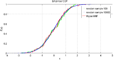
Figure 3: Cumulative density function of 100 values of the spid computed using HyperANF on cnr-2000. For comparison, we also plot random samples of size $100$ and $10\,000$ drawn from a normal distribution.

We obtained analogous concentration results for the average distance. In some pathological cases, the distribution is not Gaussian, albeit it always turns out to be unimodal (in some cases, discarding few outliers), so we can apply the Vysochanskiĭ-Petunin inequality. We will report some relevant observations on the spid of a number of graphs after describing our experiments.

6 Experiments

We ran our experiments on the datasets described in Table 2:

• the web graphs are almost all available at http://law.dsi.unimi.it/, except for the altavista dataset that was provided by Yahoo! within the Webscope program (AltaVista webpage connectivity dataset, version 1.0, http://research.yahoo.com/Academic_Relations);

• for the social networks: hollywood (http://www.imdb.com/) is a co-actorship graph where vertices represent actors; dblp (http://www.informatik.uni-trier.de/~ley/db/) is a scientific collaboration network where each vertex represents a scientist and two vertices are connected if they have worked together on an article; in ljournal (http://www.livejournal.com/) nodes are users and there is an arc from $x$ to $y$ if $x$ registered $y$ among his friends (it is not necessary to ask $y$ permission, so the graph is directed); amazon (http://www.archive.org/details/amazon_similarity_isbn/) describes similarity among books as reported by the Amazon store; enron is a partially anonymised corpus of e-mail messages exchanged by some Enron employees (nodes represent people and there is an arc from $x$ to $y$ whenever $y$ was the recipient of a message sent by $x$); finally in flickr (http://www.flickr.com/) vertices correspond to Flickr users and there is an edge connecting $x$ and $y$ whenever either vertex is recorded as a contact of the other one.

At the best of our knowledge, this is the first paper where such a wide and diverse set of data is studied, and where features such as effective diameter or average path length are computed on very large graphs with precise statistical guarantees.

Graph	snap	HyperANF
amazon	9.5 m	5 s
indochina-2004	4.62 h	1.83 m
altavista	-	1.2 h
	HADI (90 machines)	HyperANF
Kronecker (177 K nodes, 2 B arcs)	30 m	2.25 m

Table 1: A comparison of the speed of snap/HADI vs. HyperANF. The tests on snap were performed on our hardware. Both algorithms were stopped at a relative increment of $0.001$. The timings of HADI on the M45 cluster are the best reported in [KTA⁺10], and both algorithms ran three iterations. We remark that a run of HyperANF on the Kronecker graph takes less than fifteen minutes on a laptop.

Name	Type	Nodes	Arcs	spid $(\pm\sigma)$	ad $(\pm\sigma)$	ied $(\pm\sigma)$	ed (2)
amazon	social (u)	$735\,323$	$5\,158\,388$	$0.76\,(\pm 0.060)$	$12.05\,(\pm 0.206)$	$15.50\,(\pm 0.433)$	$[14\,\mathpunct{\ldotp\ldotp}18]$
dblp	social (u)	$326\,186$	$1\,615\,400$	$0.36\,(\pm 0.034)$	$7.34\,(\pm 0.114)$	$8.96\,(\pm 0.215)$	$[8\,\mathpunct{\ldotp\ldotp}10]$
enron	social (d)	$69\,244$	$276\,143$	$0.21\,(\pm 0.020)$	$4.24\,(\pm 0.065)$	$4.94\,(\pm 0.103)$	$[4\,\mathpunct{\ldotp\ldotp}6]$
ljournal	social (d)	$5\,363\,260$	$79\,023\,142$	$0.21\,(\pm 0.023)$	$5.99\,(\pm 0.078)$	$6.92\,(\pm 0.143)$	$[6\,\mathpunct{\ldotp\ldotp}8]$
flickr	social (u)	$526\,606$	$47\,097\,454$	$0.14\,(\pm 0.009)$	$3.50\,(\pm 0.047)$	$3.92\,(\pm 0.049)$	$[3\,\mathpunct{\ldotp\ldotp}5]$
hollywood	social (u)	$1\,139\,905$	$113\,891\,327$	$0.14\,(\pm 0.012)$	$3.87\,(\pm 0.045)$	$4.42\,(\pm 0.109)$	$[4\,\mathpunct{\ldotp\ldotp}5]$
indochina-2004-hosts	host (d)	$19\,123$	$233\,380$	$0.35\,(\pm 0.021)$	$4.26\,(\pm 0.079)$	$5.44\,(\pm 0.164)$	$[5\,\mathpunct{\ldotp\ldotp}7]$
uk-2005-hosts	host (d)	$587\,205$	$12\,825\,465$	$0.30\,(\pm 0.018)$	$5.93\,(\pm 0.081)$	$7.06\,(\pm 0.151)$	$[6\,\mathpunct{\ldotp\ldotp}8]$
cnr-2000	web (d)	$325\,557$	$3\,216\,152$	$2.50\,(\pm 0.086)$	$17.35\,(\pm 0.313)$	$25.45\,(\pm 0.357)$	$[23\,\mathpunct{\ldotp\ldotp}29]$
eu-2005	web (d)	$862\,664$	$19\,235\,140$	$1.25\,(\pm 0.209)$	$10.17\,(\pm 0.363)$	$14.31\,(\pm 0.988)$	$[13\,\mathpunct{\ldotp\ldotp}16]$
in-2004	web (d)	$1\,382\,908$	$16\,917\,053$	$1.30\,(\pm 0.173)$	$15.40\,(\pm 0.374)$	$20.74\,(\pm 0.792)$	$[20\,\mathpunct{\ldotp\ldotp}24]$
indochina-2004	web (d)	$7\,414\,866$	$194\,109\,311$	$1.64\,(\pm 0.134)$	$15.63\,(\pm 0.338)$	$21.68\,(\pm 0.658)$	$[20\,\mathpunct{\ldotp\ldotp}26]$
uk@10E6	web (d)	$100\,000$	$3\,050\,615$	$1.64\,(\pm 0.111)$	$5.97\,(\pm 0.172)$	$10.36\,(\pm 0.251)$	$[8\,\mathpunct{\ldotp\ldotp}12]$
uk@10E7	web (d)	$1\,000\,000$	$41\,247\,159$	$1.76\,(\pm 0.043)$	$8.96\,(\pm 0.172)$	$14.31\,(\pm 0.341)$	$[12\,\mathpunct{\ldotp\ldotp}17]$
it-2004	web (d)	$41\,291\,594$	$1\,150\,725\,436$	$2.14\,(\pm 0.149)$	$15.02\,(\pm 0.300)$	$19.65\,(\pm 0.698)$	$[18\,\mathpunct{\ldotp\ldotp}22]$
uk-2007-05	web (d)	$105\,896\,555$	$3\,738\,733\,648$	$1.10\,(\pm 0.234)$	$15.39\,(\pm 0.418)$	$19.93\,(\pm 1.030)$	$[18\,\mathpunct{\ldotp\ldotp}23]$
altavista	web (d)	$1\,413\,511\,390$	$6\,636\,600\,779$	$4.24\,(\pm 0.764)$	$16.69\,(\pm 0.779)$	$23.04\,(\pm 2.517)$	$[19\,\mathpunct{\ldotp\ldotp}31]$

Table 2: Our main data table. “Type” describes whether the given graph is a web-graph, a proper social network, or the host quotient of a web graph (u=undirected, d=directed). The graphs uk@10E6 and uk@10E7 are obtained by visiting in a breadth-first fashion uk-2007-05 starting from a random node. They simulate smaller crawls of a larger network. We show spid, average distance and interpolated effective diameter a posteriori with their empirical standard deviation, and intervals for the effective diameter with $85$% confidence for a comparison.

All experiments are performed on a Linux server equipped with Intel Xeon X5660 CPUs ($2.80$ GHz, $12$ MB cache size) for overall 24 cores and $128$ GB of RAM; the server cost about $8\,900$ EUR in 2010.

A brief comparison with snap and HADI timings is shown in Table 1. Essentially, on our hardware HyperANF is two orders of magnitudes faster than snap. Our run on the Kronecker graph is one order of magnitude faster than HADI’s (or three orders of magnitude faster, if you take into consideration the number of machines involved), but this comparison is unfair, as in principle HADI can scale to arbitrarily large graphs, whereas we are limited by the amount of memory available. Nonetheless, the speedup is clearly a breakthrough in the analysis of large graphs. It would be interesting to compare our timings for the altavista dataset with HADI’s, but none have been published.

It is this speed that makes it possible, for the first time, to compute data associated with the distance distribution with high precision and for a large number of graphs. We have 100 runs with relative standard deviation of $9.37$% for all graphs, except for those on the altavista dataset ($13.25$%). All graphs are run to stabilisation. Our computations are necessarily much longer (usually, an order of magnitude longer in iterations) than those used to compute the effective diameter or similar measures. This is due to the necessity of computing with high precision second-order statistics that are used to compute the spid.

Previous publications used few graphs, mainly because of the large computational effort that was necessary, and no data was available about the number of runs. Moreover, we give precise confidence intervals based on parametric statistics for data depending on the second moment, such as the spid—something that has never done before. We gather here our findings.

A posteriori parameters are highly concentrated. According to our experiments, computing the effective diameter, average distance and spid on a large number of low-precision runs generates highly concentrated distributions (see the empirical standard deviation in Table 2). Thus, we suggest this approach for computing such values, provided that termination is by stabilisation.

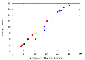
Figure 4: A plot showing the strong linear correlation between the average distance and the effective diameter.

Effective diameter and average distance are essentially linearly correlated. Figure 4 shows a scatter plot of the two values, and the line $2x/3+1$. The correlation between the two values has always been folklore in the study of social networks, but we can confirm that on both social and web networks the connection can be exactly expressed in linear terms (it would be of course interesting to prove such a correlation formally, under suitable restrictions on the structure of the graph). This fact suggests that the average distance (which is more principled from a statistic viewpoint, and parameter-free) should be used as the reference parameter to express the closeness between nodes. Moreover, experimentally the standard deviation of the effective diameter in a posteriori computations is usually significantly larger than that of the average distance.

Incidentally, the average distance of the altavista dataset is $16.5$—slightly more than what reported in [KTA⁺10] (possibly because of termination conditions artifacts).

It is difficult to give a priori confidence intervals for the effective diameter with a small number of runs. Unless a large number of runs is available, so that the precision of the approximation of the neighbourhood function can be significantly lowered, it is impossible to provide interesting upper bounds for the effective diameter.

The spid can tell social networks from web graphs. As shown in Table 2, even taking the standard deviation into account spids are pretty much below 1 for social networks and above 1 for web graphs; host graphs (not surprisingly) behave like social networks. Note that this works both for directed and undirected graphs. Figure 5 shows the spid values obtained for our datasets plotted against the graph size, and also witnesses that there is no correlation (a similar graph, not shown here, testifies that spid is also independent from density). Figure 6 shows that there is some slight correlation between the spid and the average distance: nonetheless, there is no way to tell networks from our dataset apart using the latter value, whereas the under- or over-dispersion of the distance distribution, as defined by the spid, never makes a mistake. Of course, we expect to enrich this graph in time with more datasets: we are particularly interested in gathering very large social networks to test the spid at large sizes.

We remark that, as a sanity check, we have also computed on several web-graph datasets the spid of the giant component, which turned out to be very similar to the spid of the whole graph. We see this as a clear sign that the spid is largely independent of the artifacts of the crawling process.

Direction should not be destroyed when analysing a graph. We confirm that symmetrising graphs destroys the combinatorial structure of the network: the average distance drops to very low values in all cases, as well as the spid. This suggests that there is important structural information that is being ignored. We also note that since all web snapshot we have at hand are gathered by some kind of breadth-first visit, they represent balls of small diameter centred at the seed: symmetrising the graph we cannot expect to get an average distance that is larger than twice the radius of the ball. All in all, the only advantage of symmetrising a graph is a significant reduction in the number of iterations that are needed to complete a computation of the neighbourhood function.

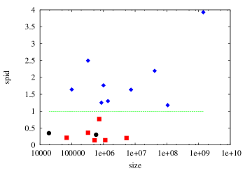
Figure 5: A plot showing the spid values (vertical) for our datasets compared with their size (i.e., number of nodes, horizontal): red squares correspond to social networks, blue diamonds to web graphs and black circles to host graphs.

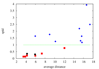
Figure 6: A plot showing the spid against the average distance using the same conventions of Figure 5.

To give a more direct idea of the level of precision of our diameter estimation, we computed the actual diameter at $\alpha$ for the cnr-2000 dataset, and plotted it against the interval estimation obtained by HyperANF

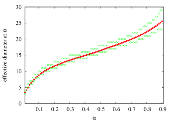
Figure 7: Effective diameters at $\alpha$ for the cnr-2000 dataset; red bullets show the real effective diameter, whereas green crosses show the upper and lower extreme of the confidence interval obtained running $100$ HyperANF with $m=128$.

7 Future work

HyperANF lends itself naturally to distributed implementations. However, contrarily to the approach taken by HADI [KTA⁺10], we think that the correct parallel framework for implementing a diffusing computation is a synchronous parallel system where computation happens at nodes and communication is sent from node to node with messages. Such a framework, Pregel, has been recently developed at Google [MAB⁺10]. In a Pregel implementation of HyperANF, every computational node sends its own counter as message to its predecessors if it changed from the previous iteration, waits for incoming messages from its successors, and computes the maximisation procedure on the received messages. Due to the small size of HyperLogLog counter (exponentially smaller than the Flajolet–Martin counters used by ANF), the amount of communication would be very small.

Although in this paper, we preferred to focus on the computation of the spid, we remark that HyperANF can also be used to build the radius distribution described in [KTA⁺10], or the related closeness centrality.

8 Conclusions

HyperANF is a breakthrough improvement over the original ANF techniques, mainly because of the usage of the more powerful HyperLogLog counters combined with their fast broadword combination and systolic computation. HyperANF can run to stabilisation very large graphs, computing data with statistical guarantees.

We consider, however, the introduction of the spid of a graph the main conceptual contribution of this paper. HyperLogLog is instrumental in making the computation of the spid possible, as the latter requires a number of iterations that is an order of magnitude larger than those required for an estimate of the effective diameter.

Acknowledgements

Flavio Chierichetti participated to the earlier phases of this work. We want to thank Dario Malchiodi for fruitful discussions and hints.

References

- [AMS99] Noga Alon, Yossi Matias, and Mario Szegedy. The space complexity of approximating the frequency moments. J. Comput. Syst. Sci, 58(1):137–147, 1999.
- [BV04] Paolo Boldi and Sebastiano Vigna. The WebGraph framework I: Compression techniques. In Proc. of the Thirteenth International World Wide Web Conference (WWW 2004), pages 595–601, Manhattan, USA, 2004. ACM Press.
- [Coh97] Edith Cohen. Size-estimation framework with applications to transitive closure and reachability. J. Comput. Syst. Sci., 55:441–453, 1997.
- [DF03] Marianne Durand and Philippe Flajolet. Loglog counting of large cardinalities (extended abstract). In Giuseppe Di Battista and Uri Zwick, editors, Algorithms - ESA 2003, 11th Annual European Symposium, Budapest, Hungary, September 16-19, 2003, Proceedings, volume 2832 of Lecture Notes in Computer Science, pages 605–617. Springer, 2003.
- [FFGM07] Philippe Flajolet, Éric Fusy, Olivier Gandouet, and Frédéric Meunier. Hyperloglog: the analysis of a near-optimal cardinality estimation algorithm. In Proceedings of the 13th conference on analysis of algorithm (AofA 07), pages 127–146, 2007.
- [HH85] J. A. Hartigan and P. M. Hartigan. The dip test of unimodality. Ann. Statist., 13(1):70–84, 1985.
- [Knu07] Donald E. Knuth. The Art of Computer Programming. Pre-Fascicle 1A. Draft of Section 7.1.3: Bitwise Tricks and Techniques, 2007.
- [KTA+10] U Kang, Charalampos E. Tsourakakis, Ana Paula Appel, Christos Faloutsos, , and Jure Leskovec. HADI: Mining radii of large graphs. ACM Transactions on Knowledge Discovery from Data, 2010.
- [MAB+10] Grzegorz Malewicz, Matthew H. Austern, Aart J.C Bik, James C. Dehnert, Ilan Horn, Naty Leiser, and Grzegorz Czajkowski. Pregel: a system for large-scale graph processing. In SIGMOD ’10: Proceedings of the 2010 international conference on Management of data, pages 135–146, New York, NY, USA, 2010. ACM.
- [PGF02] Christopher R. Palmer, Phillip B. Gibbons, and Christos Faloutsos. Anf: a fast and scalable tool for data mining in massive graphs. In KDD ’02: Proceedings of the eighth ACM SIGKDD international conference on Knowledge discovery and data mining, pages 81–90, New York, NY, USA, 2002. ACM.
- [Vig07] Sebastiano Vigna. Stanford matrix considered harmful. In Andreas Frommer, Michael W. Mahoney, and Daniel B. Szyld, editors, Web Information Retrieval and Linear Algebra Algorithms, number 07071 in Dagstuhl Seminar Proceedings, 2007. http://arxiv.org/abs/0710.1962.
- [Vig08] Sebastiano Vigna. Broadword implementation of rank/select queries. In Catherine C. McGeoch, editor, Experimental Algorithms. 7th International Workshop, WEA 2008, number 5038 in Lecture Notes in Computer Science, pages 154–168. Springer–Verlag, 2008.
- [VP82] D. F. Vysochanskiĭ and Yu. Ī. Petunīn. Remark: “Proof of the rule for unimodal distributions” [Teor. Veroyatnost. i Mat. Statist. 21 (1979), 23–35]. Teor. Veroyatnost. i Mat. Statist., 27:26–27, 157, 1982.