Dissipative dynamics of two-qubit system: four-level lasing

Abstract

The dissipative dynamics of a two-qubit system is studied theoretically. We make use of the Bloch-Redfield formalism which explicitly includes the parameter-dependent relaxation rates. We consider the case of two flux qubits, when the controlling parameters are the partial magnetic fluxes through the qubits’ loops. The strong dependence of the inter-level relaxation rates on the controlling magnetic fluxes is demonstrated for the realistic system. This allows us to propose several mechanisms for lasing in this four-level system.

I Introduction

Recently considerable progress has been made in studying Josephson-junctions-based superconducting circuits, which can behave as effectively few-level quantum systems. Korotkov When the dynamics of the system can be described in terms of two levels only, this circuit is called a qubit. Demonstrations of the energy level quantization and the quantum coherence provide the basis for both possible practical applications and for studying fundamental quantum phenomena in systems involving qubits. Important distinctions of these multi-level artificial quantum systems from their microscopic counterparts are high level of controllability and unavoidable coupling to the dissipative environment.

Multi-level systems with solid-state qubits may be realized in different ways. First, the devices used for qubits in reality are themselves multi-level systems with the lowest two levels used to form a qubit. For some recent study of multi-level superconducting devices see Ref. 1-qb-multilevel, . Then, a qubit can be coupled to another quantum system, e.g. a quantum resonator.qb-oscillator Such a composite system is also described by a multi-level structure. As a particular case of coupling with other systems, the multi-qubit system is of particular interest (see e.g. Ref. 2qbs, ).

Operations with the multi-level systems can be described with level-population dynamics. In particular, population inversion was proposed for cooling and lasing with superconducting qubits.Astafiev07 ; Grajcar08-i-drugie However, most of the previous propositions were related to three-level systems, while for practical purposes four-level systems are often more advantageous.Svelto

The natural candidate for the solid-state four-level system is the system of two coupled qubits. The purpose of this paper is the theoretical study of mechanisms of population inversion and lasing, as a result of the pumping and relaxation processes in the system. We will start in the next Section by demonstrating the controllable energy level structure of the system. Our calculations are done for the parameters of the realistic two-flux-qubit system studied in Ref. Ilichev10, . To describe the dynamics of the system we will present the Bloch-Redfield formalism in Sec. III. The key feature of the system is the strong dependence of the relaxation rates on the controlling parameters. Then solving the master equation in Sec. IV we will demonstrate several mechanisms for creating the population inversion in our four-level system. We will demonstrate further that applying additional driving induces transitions between the operating states resulting in stimulated emission. We summarize our theoretical results in Sec. V. and, based on our calculations, we then discuss the experimental feasibility of the two-qubit lasing.

II Model Hamiltonian and Eigenstates of the two-qubit system

The main object of our study is a system of two coupled qubits. And altough our analysis bears general character, for concreteness we consider superconducting flux qubits, see Fig. 1. A flux qubit, which is a superconducting ring with three Josephson junctions, can be controlled by constant ($\Phi_{\mathrm{dc}}$) and alternating ($\Phi_{\mathrm{ac}}\sin\omega t$) external magnetic fluxes. Each of the two qubits can be considered as a two-level system with the Hamiltonian in the pseudospin notation vanderWal03 ; Korotkov

$$\widehat{H}_{\mathrm{1q}}^{(i)}=-\frac{1}{2}\epsilon_{i}(t)\widehat{\sigma}_{z}^{(i)}-\frac{1}{2}\Delta_{i}\widehat{\sigma}_{x}^{(i)},$$ (1)

where $\Delta_{i}$ is the tunnelling amplitude, $\widehat{\sigma}_{x,z}^{(i)}$ are the Pauli matrices in the basis $\left\{\lvert{\downarrow}\rangle,\lvert{\uparrow}\rangle\right\}$ of the current operator in the $i$-th qubit: $\widehat{I}_{i}=-I_{\mathrm{p}}^{(i)}\widehat{\sigma}_{z}^{(i)},$ with $I_{\mathrm{p}}^{(i)}$ being the absolute value of the persistent current in the $i$-th qubit; then the eigenstates of $\widehat{\sigma}_{z}$ correspond to the clockwise ($\widehat{\sigma}_{z}\left|\downarrow\right\rangle=-\left|\downarrow\right\rangle$) and counterclockwise ($\widehat{\sigma}_{z}\left|\uparrow\right\rangle=\left|\uparrow\right\rangle$) current in the $i$-th qubit. The energy bias $\epsilon_{i}(t)$ is controlled by constant and alternating magnetic fluxes

$$\epsilon_{i}(t) = 2I_{\mathrm{p}}^{(i)}\left(\Phi_{i}(t)-\frac{1}{2}\Phi_{0}\right)=\epsilon_{i}^{(0)}+\tilde{\epsilon}_{i}(t),$$ (2a)

$$\epsilon_{i}^{(0)} = 2I_{\mathrm{p}}^{(i)}\Phi_{0}f_{i}\text{, \ \ }f_{i}=\frac{\Phi_{\mathrm{dc}}^{(i)}}{\Phi_{0}}-\frac{1}{2},$$ (2b)

$$\tilde{\epsilon}_{i}(t) = 2I_{\mathrm{p}}^{(i)}\Phi_{0}f_{\mathrm{ac}}\sin\omega t\text{, \ \ }f_{\mathrm{ac}}=\frac{\Phi_{\mathrm{ac}}}{\Phi_{0}}.$$ (2c)

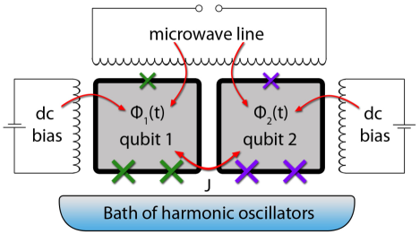
Figure 1: (Color online). Schematic diagram of the two-qubit system. Two different flux qubits are biased by independent constant magnetic fluxes, $\Phi_{\mathrm{dc}}^{(1)}$ and $\Phi_{\mathrm{dc}}^{(2)}$, and by the same alternating magnetic flux $\Phi_{\mathrm{ac}}\sin\omega t$. The former controls the energy levels structure, while the latter changes the populations of the levels. The dissipation processes are described by coupling the system to the bath of harmonic oscillators.

The basis state vectors for the two-qubit system $\left\{\lvert{\downarrow\downarrow}\rangle,\lvert{\downarrow\uparrow}\rangle,\lvert{\uparrow\downarrow}\rangle,\lvert{\uparrow\uparrow}\rangle\right\}$ are composed from the single-qubit states: $\lvert{\downarrow\uparrow}\rangle=\lvert{\downarrow}\rangle_{(1)}\lvert{\uparrow}\rangle_{(2)}$, etc. For identification of the level structure and understanding different transition rates, we will start the consideration from the case of two non-interacting qubits. Then, the energy levels of two qubits consist of the pair-wise summation of single-qubit levels,

$$E_{i}^{\pm}=\pm\frac{\Delta E_{i}}{2}=\pm\frac{1}{2}\sqrt{\epsilon_{i}^{(0)2}+\Delta_{i}^{2}},$$ (3)

which are the eigenstates of the single-qubit time-independent Hamiltonian (1) at $f_{\mathrm{ac}}=0$. We demonstrate this in Fig. 2(a), where we plot the energy levels, fixing the bias in the first qubit $f_{1}$, as a function of the partial bias in the second qubit $f_{2}$. Then the single-qubit energy levels appear as (dashed) horizontal lines at $E_{1}^{\pm}=\pm\frac{1}{2}\sqrt{\epsilon_{1}^{(0)2}+\Delta_{1}^{2}}$ for the first qubit and as the parabolas at $E_{2}^{\pm}(f_{2})=\pm\frac{1}{2}\sqrt{\epsilon_{2}^{(0)}(f_{2})^{2}+\Delta_{2}^{2}}$.

After showing the two-qubit energy levels in Fig. 2(a), we assume that the relaxation in the first qubit is much faster than in the second (this will be studied in the next Section), which is shown with the arrows in the figure. And now our problem, with four levels and with fast relaxation between certain levels, becomes similar to the one with lasers. Svelto This allows us to propose three- and four-level lasing schemes in Fig. 2(b,c). This is the subject of our further detailed study.

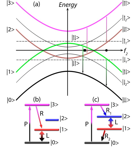
Figure 2: (Color online). Energy level structure of two uncoupled qubits ($J=0$). (a) One-qubit and two-qubits energy levels are shown by dashed and solid lines as a function of partial flux $f_{\mathrm{2}}$ at fixed flux $f_{\mathrm{1}}$. We mark the energy levels by the current operator eigenstates, $\lvert{\downarrow\downarrow}\rangle$ etc. Particularly, we will consider the energy levels and dynamical behaviour of the system for the flux biases $f_{\mathrm{2}}=f_{2\mathrm{L}}$ (marked by the square) and $f_{\mathrm{2}}=f_{2\mathrm{R}}$ (marked by the circle). By the arrows we show the fastest relaxation - for qubit $1$. (b) Scheme for three-level lasing at $f_{\mathrm{2}}=f_{2\mathrm{L}}$. The driving magnetic flux pumps (P) the upper level $\left|3\right\rangle$. Fast relaxation (R) creates the population inversion of the first excited level $\left|1\right\rangle$ in respect to the ground state $\left|0\right\rangle$; these two operating levels can be used for lasing (L). (c) Scheme for four-level lasing at $f_{\mathrm{2}}=f_{2\mathrm{R}}$. Pumping (P) and fast relaxations (R₁ and R₂) create the population inversion of the level $\left|2\right\rangle$ with respect to level $\left|1\right\rangle$.

We have analyzed the relaxation in the system of two uncoupled qubits. However this system can not be used for lasing, since this requires pumping from the ground state to the upper excited state (see Fig. 2(b,c)). Such excitation of the two-qubit system requires simultaneously changing the state of both qubits and can be done provided the two qubits are interacting. That is why in what follows we consider in detail the system of two coupled qubits. The coupling between the two qubits we assume to be determined by an Ising-type (inductive interaction) term $\frac{J}{2}\widehat{\sigma}_{z}^{(1)}\widehat{\sigma}_{z}^{(2)}$, where $J$ is the coupling energy between the qubits. Then the Hamiltonian of the two driven flux qubits can be represented as the sum of time-independent and perturbation Hamiltonians

$$\widehat{H}_{\mathrm{2q}}=\widehat{H}_{0}+\widehat{V}(t),$$ (4)

$$\widehat{H}_{0}=\sum_{i=1,2}\left(-\frac{1}{2}\Delta_{i}\widehat{\sigma}_{x}^{(i)}-\frac{1}{2}\epsilon_{i}^{(0)}\widehat{\sigma}_{z}^{(i)}\right)+\frac{J}{2}\widehat{\sigma}_{z}^{(1)}\widehat{\sigma}_{z}^{(2)},$$ (5)

$$\widehat{V}(t)=\sum_{i=1,2}-\frac{1}{2}\tilde{\epsilon}_{i}(t)\widehat{\sigma}_{z}^{(i)},$$ (6)

where $\widehat{\sigma}_{x,z}^{(1)}=\widehat{\sigma}_{x,z}\otimes\widehat{\sigma}_{0}$, $\widehat{\sigma}_{x,z}^{(2)}=\widehat{\sigma}_{0}\otimes\widehat{\sigma}_{x,z}$, and $\widehat{\sigma}_{0}$ is the unit matrix. When presenting concrete results we will use the parameters of Ref. Ilichev10, : $\Delta_{\mathrm{1}}/h=15.8$ GHz, $\Delta_{\mathrm{2}}/h=3.5$ GHz, $I_{\mathrm{p}}^{(\mathrm{1})}\Phi_{0}/h=375$ GHz, $I_{\mathrm{p}}^{(\mathrm{2})}\Phi_{0}/h=700$ GHz, $J/h=3.8$ GHz.

For further analysis of the system, we have to convert to the basis of eigenstates of the unperturbed Hamiltonian (5). Eigenstates $\left\{\lvert{0}\rangle,\lvert{1}\rangle,\lvert{2}\rangle,\lvert{3}\rangle\right\}$ of the unperturbed Hamiltonian (5) are connected with the initial basis

$$\left[\begin{matrix}\lvert{0}\rangle\\ \lvert{1}\rangle\\ \lvert{2}\rangle\\ \lvert{3}\rangle\end{matrix}\right]=\widehat{S}\left[\begin{matrix}\lvert{\downarrow\downarrow}\rangle\\ \lvert{\downarrow\uparrow}\rangle\\ \lvert{\uparrow\downarrow}\rangle\\ \lvert{\uparrow\uparrow}\rangle\end{matrix}\right],$$ (7)

where $\widehat{S}$ is the unitary matrix consisting of eigenvectors of the unperturbed Hamiltonian (5). Making use of the transformation $\widehat{H}_{0}^{\prime}=\widehat{S}^{-1}\widehat{H}_{0}\widehat{S}$, we obtain the Hamiltonian $\widehat{H}_{0}^{\prime}$ in the energy representation: $\widehat{H}_{0}^{\prime}=$diag$(E_{0},E_{1},E_{2},E_{3})$. These eigenvalues of the Hamiltonian $H_{0}$ are computed numerically and plotted in Fig. 3(a) as functions of the bias flux in the second qubit $f_{2}$. The distinction from Fig. 2(a), calculated with $J=0$, is in that, first, the crossing at $f_{2}=f_{2}^{\ast}$ becomes an avoided crossing, and second, the distance between the [previously single-qubit] energy levels is not equal, e.g. now $E_{3}-E_{2}\neq E_{1}-E_{0}$.

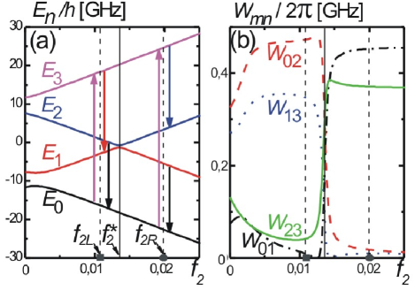
Figure 3: (Color online). (a) Energy levels of the system of two coupled qubits. Arrows show the pumping and dominant relaxation, as in Fig. 2. (b) The relaxation rates $W_{mn}$, which give the probability of the transition from level $n$ to level $m$, induced by the interaction with the dissipative bath. Dominant relaxations are $W_{13}$ and $W_{02}$ to the left from the avoided crossing at $f_{\mathrm{2}}=f_{\mathrm{2}}^{\ast}$ and $W_{23}$ and $W_{01}$ to the right. (The small relaxation rates $W_{03}$ and $W_{12}$ are not shown.)

Likewise, we could also convert the excitation operator $\widehat{V}(t)$ to the energy representation

$$\widehat{V}^{\prime}(t)=\widehat{S}^{-1}\widehat{V}(t)\widehat{S}=\sum_{i=1,2}-\frac{1}{2}\tilde{\epsilon}_{i}(t)\widehat{\tau}_{z}^{(i)},$$ (8)

$$\widehat{\tau}_{z}^{(i)}=\widehat{S}^{-1}\widehat{\sigma}_{z}^{(i)}\widehat{S}.$$ (9)

III Master equation and relaxation

III.1 Bloch-Redfield formalism

Following Ref. MasterEqn, , we will describe the dissipation in the open system of two qubits, assuming that it is interacting with the thermostat (bath), see Fig. 1. Within the Bloch-Redfield formalism, the Liouville equation for the quantum system interacting with the bath is transformed into the master equation for the reduced system’s density matrix. This transformation is made with several reasonable assumptions: the interaction with the bath is weak (Born approximation); the bath is so large that the effect of the system on its state is ignored; the dynamics of the system depends on its state only at present (Markov approximation). Then the master equation for the reduced density matrix $\rho(t)$ of our driven system in the energy representation can be written in the form of the following differential equations MasterEqn

$$\dot{\rho}_{ij}=-i\omega_{ij}\rho_{ij}-\frac{i}{\hbar}\left[\widehat{V}^{\prime},\widehat{\rho}\right]_{ij}+\delta_{ij}\sum_{n\neq j}\rho_{nn}W_{jn}-\gamma_{ij}\rho_{ij}.$$ (10)

Here $\omega_{ij}=(E_{i}-E_{j})/\hbar$, and the relaxation rates

$$W_{mn}=2\text{Re}\Gamma_{nmmn},$$ (11)

$$\gamma_{mn}=\sum_{r}\left(\Gamma_{mrrm}+\Gamma_{nrrn}^{\ast}\right)-\Gamma_{nnmm}-\Gamma_{mmnn}^{\ast}$$ (12)

are defined by the relaxation tensor $\Gamma_{lmnk}$, which is given by the Golden Rule

$$\Gamma_{lmnk}=\frac{1}{\hbar^{2}}\int\limits_{0}^{\infty}dte^{-i\omega_{nk}t}\left\langle H_{\mathrm{I},lm}(t)H_{\mathrm{I},nk}(0)\right\rangle.$$ (13)

Here $\widehat{H}_{\mathrm{I}}(t)$ is the Hamiltonian of the interaction of our system with the bath in the interaction representation; the angular brackets denote the thermal averaging of the bath degrees of freedom.

It was shown vanderWal03 ; Governale01-i-drugie that the noise from the electromagnetic circuitry can be described in terms of the impedance $Z(\omega)$ from a bath of $LC$ oscillators. For simplicity one assumes that both qubits are coupled to a common bath of oscillators, then the Hamiltonian of interaction is written as

$$\widehat{H}_{\mathrm{I}}=\frac{1}{2}\left(\widehat{\sigma}_{z}^{(1)}+\widehat{\sigma}_{z}^{(2)}\right)\widehat{X}$$ (14)

in terms of the collective bath coordinate $\widehat{X}=\sum\nolimits_{k}c_{k}\widehat{\Phi}_{k}$. Here $\widehat{\Phi}_{k}$ stands for the magnetic flux (generalized coordinate) in the $k$-th oscillator, which is coupled with the strength $c_{k}$ to the qubits. We note that the coupling to the environment in the form of Eq. (14) applies only to correlated noise, or both qubits interacting with the same environment. One could argue that it would be more realistic to use two separate terms, one for each qubit coupled to its own environment. However, since this term leads to different relaxation rates in our qubits $1$ and $2$ (see below), then the form in Eq. (14) should give essentially the same results as two separate coupling terms.

Then it follows that the relaxation tensor $\Gamma_{lmnk}$ is defined by the noise correlation function $S(\omega)$

$$\Gamma_{lmnk}=\frac{1}{\hbar^{2}}\Lambda_{lmnk}S(\omega_{nk}),$$ (15)

$$\Lambda_{lmnk}=\left(\widehat{\tau}_{z}^{(1)}+\widehat{\tau}_{z}^{(2)}\right)_{lm}\left(\widehat{\tau}_{z}^{(1)}+\widehat{\tau}_{z}^{(2)}\right)_{nk},$$ (16)

$$S(\omega)=\int\limits_{0}^{\infty}dte^{-i\omega t}\left\langle X(t)X(0)\right\rangle.$$ (17)

The noise correlator $S(\omega)$ was calculated in Ref. Governale01-i-drugie, within the spin-boson model and it was shown that its imaginary part results only in a small renormalization of the energy levels and can be neglected. The relevant real part of the relaxation tensor Governale01-i-drugie

$$\text{Re}\Gamma_{lmnk}=\frac{1}{8\hbar}\Lambda_{lmnk}J(\omega_{nk})\left[\coth\frac{\hbar\omega_{nk}}{2T}-1\right]$$ (18)

is defined by the environmental spectral density $J(\omega)$. Here $T$ is the bath temperature ($k_{B}$ is assumed $1$); for the numerical calculations we take $T/h=1$ GHz ($T=50$ mK). The electromagnetic environment can be described as an Ohmic resistive shunt across the junctions of the qubits, $Z(\omega)=R$.vanderWal03 Then the low frequency spectral density is linear $J(\omega)\propto\omega Z(\omega)\propto$ $\omega$ and should be cut off at some large value $\omega_{\mathrm{c}}$; the realistic experimental situation is described by Governale01-i-drugie

$$J(\omega)=\alpha\frac{\hbar\omega}{1+\omega^{2}/\omega_{\mathrm{c}}^{2}},$$ (19)

where $\alpha$ is a dimensionless parameter that describes the strength of the dissipative effects; in numerical calculations we take $\alpha=0.01$ and $\omega_{\mathrm{c}}/2\pi=10^{4}$ GHz (the cut-off frequency $\omega_{\mathrm{c}}$ is taken much larger than other characteristic frequencies, so that for relevant values $\omega:$ $J(\omega)\approx\alpha\hbar\omega$).

III.2 Relaxation rates

From the above equations the expression for the relaxation rates from level $\left|n\right\rangle$ to level $\left|m\right\rangle$ follows

$$W_{mn}=\frac{1}{4\hbar}\Lambda_{nmmn}J(\omega_{mn})\left[\coth\frac{\hbar\omega_{mn}}{2T}-1\right].$$ (20)

These relaxation rates are plotted in Fig. 3(b) as functions of the partial flux bias $f_{2}$. This figure demonstrates that the fastest transitions are those between the energy levels corresponding to changing the state of the first qubit and leaving the same state of the second qubit, cf. Fig. 3(a). Namely, the fastest transitions are those with the rates $W_{13}$ and $W_{02}$ to the left from the avoided crossing and $W_{23}$ and $W_{01}$ to the right, which correspond to the transitions $\lvert{\uparrow\uparrow}\rangle\rightarrow\lvert{\downarrow\uparrow}\rangle$ and $\lvert{\uparrow\downarrow}\rangle\rightarrow\lvert{\downarrow\downarrow}\rangle$. Note that we do not show in the figure the rates $W_{03}$ and $W_{12}$; they correspond to the transitions with simultaneously changing the states of the two qubits and they are much smaller than the rates shown.

The relaxation rates $W_{ij}$ are shown in Fig. 4 as functions of the two partial bias fluxes, $f_{1}$ and $f_{2}$. Again, one can see the regions where certain relaxation rates are dominant. Such a difference in the relaxation rates creates a sort of artificial selection rules for the transitions similar to the selection rules studied in Refs. Liu05, ; deGroot, . In our case the transitions are induced by the interaction with the environment and the difference is due to the different parameters of the two qubits.Paladino09 To further understand this issue, we consider the single-qubit relaxation rates.

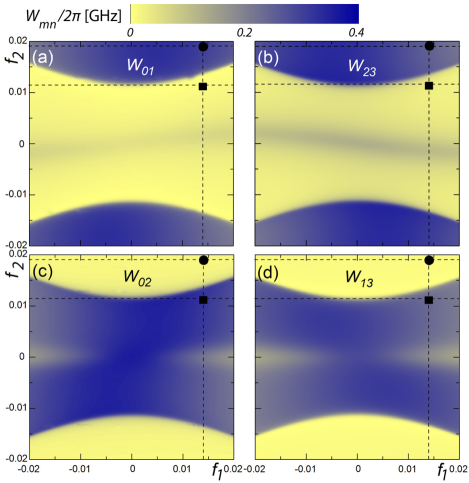
Figure 4: (Color online). Relaxation rates $W_{mn}$ versus partial biases of the two qubits, $f_{\mathrm{1}}$ and $f_{\mathrm{2}}$. The square and the circle show the parameters $f_{\mathrm{1}}$ and $f_{\mathrm{2}}=f_{\mathrm{2L(R)}}$, at which the calculations of other figures are done.

From the above equations we can obtain the energy relaxation time $T_{1}$ and the decoherence time $T_{2}$ for single qubit. For the two-level system with two states $\lvert{0}\rangle$ and $\lvert{1}\rangle$ the relaxation time is given by MasterEqn $T_{1}^{-1}=W_{01}+W_{10}$. The Boltzmann distribution, $W_{10}/W_{01}=\exp(-\Delta E/T)$, means that at low temperature the major effect of the bath is the relaxation from the upper level to the lower one. Now, from Eq. (20) it follows that

$$T_{1}^{-1}=\frac{\alpha\Delta^{2}}{2\hbar\Delta E}\coth\frac{\Delta E}{2T}.$$ (21)

Also from Eq. (12) we obtain the dephasing rate MasterEqn

$$T_{2}^{-1}=\text{Re}\gamma_{01}=\frac{1}{2}T_{1}^{-1}+\frac{\alpha T}{\hbar}\frac{\epsilon^{(0)2}}{\Delta E^{2}}.$$ (22)

For the calculation presented in Fig. 2(a) for two qubits with $J=0$ in the vicinity of the point $f_{2}=f_{2}^{\ast}$, where $\Delta E^{(1)}=\Delta E^{(2)}$, we obtain

$$\frac{T_{1}^{(1)}}{T_{1}^{(2)}}\simeq\left(\frac{\Delta_{2}}{\Delta_{1}}\right)^{2}.$$ (23)

As we explained above, the lasing in the four-level system requires the hierarchy of the relaxation times. In particular, we assumed $T_{1}^{(1)}\ll T_{1}^{(2)}$. So, in our calculations we have taken $\Delta_{1}\gg\Delta_{2}$ and consequently the first qubit relaxed faster. This qualitatively explains the dominant relaxations in Fig. 3(b).

III.3 Equations for numerical calculations

If we use the Hermiticity and normalization of the density matrix, then the $16$ complex equations (10) can be reduced to $15$ real equations. After the straightforward parametrization of the density matrix, $\rho_{ij}=x_{ij}+iy_{ij}$, we get ShT08

$$\dot{x}_{ii}=-\frac{1}{\hbar}\left[V^{\prime},y\right]_{ii}+\sum_{r\neq i}W_{ir}x_{rr}-x_{ii}\sum_{r\neq i}W_{ii},\text{ }i=1,2,3;$$ (24a)

$$\dot{x}_{ij}=\omega_{ij}y_{ij}-\frac{1}{\hbar}\left[V^{\prime},y\right]_{ij}-\gamma_{ij}x_{ij},\text{ }i>j;$$ (24b)

$$\dot{y}_{ij}=-\omega_{ij}x_{ij}+\frac{1}{\hbar}\left[V^{\prime},y\right]_{ij}-\gamma_{ij}y_{ij},\text{ }i>j;$$ (24c)

$$y_{ii}=0 x_{00}=1-(x_{11}+x_{22}+x_{33}) x_{ji}=x_{ij} y_{ji}=-y_{ij}$$, ; , .

This system of equations can be simplified if the relaxation rates are taken at zero temperature, $T=0$, and neglecting the impact of the inter-qubit interaction on relaxation, $J=0$. Then among all the $W_{ij}$ and $\gamma_{ij}$ non-trivial are only the elements corresponding to single-qubit relaxations (see Eqs. (21-22)). For example consider $f_{2}<f_{2}^{\ast}$ (see Fig. 2(a) for the notation of the levels), then non-trivial elements are

$$W_{13} = W_{02}=\left(T_{1}^{(1)}\right)^{-1}=\frac{\alpha\Delta_{1}^{2}}{2\hbar\Delta E_{1}},$$ (25a)

$$W_{23} = W_{01}=\left(T_{1}^{(2)}\right)^{-1}=\frac{\alpha\Delta_{2}^{2}}{2\hbar\Delta E_{2}},$$ (25b)

$$\gamma_{13} = \gamma_{31}=\gamma_{02}=\gamma_{20}=(T_{2}^{(1)})^{-1}=\frac{1}{2}(T_{1}^{(1)})^{-1},$$ (26a)

$$\gamma_{23} = \gamma_{32}=\gamma_{01}=\gamma_{10}=(T_{2}^{(2)})^{-1}=\frac{1}{2}(T_{1}^{(2)})^{-1}.$$ (26b)

In our numerical calculations we did not ignore the influence of the coupling on relaxation, i.e. we did not assume $J=0$. However, we have numerically checked that such simplification, $J=0$, resulting in the relaxation rates (25-26), sometimes allows to describe qualitatively dynamics of the system.

IV Several schemes for lasing

In Sec. II and in Fig. 2 we pointed out that in the system of two coupled qubits there are two ways to realize lasing, making use of the three or four levels to create the population inversion between the operating levels. In this Section we will demonstrate the lasing in the two-qubit system solving numerically the Bloch-type equations (24) with the relaxation rates given by Eqs. (11, 12, 18). Besides demonstrating the population inversion between the operating levels, we apply an additional signal with the frequency matching the distance between the operating levels, to stimulate the transition from the upper operating level to the lower one. So, we will first consider the system driven by one monochromatic signal $f(t)=f_{\mathrm{ac}}\sin\omega t$ to pump the system to the upper level and to demonstrate the population inversion. Then we will apply another signal stimulating transitions between the operating laser levels:

$$f(t)=f_{\mathrm{ac}}\sin\omega t+f_{\mathrm{L}}\sin\omega_{\mathrm{L}}t.$$ (27)

Solving the system of equations (24), we obtain the population of $i$-th level of our two-qubit system, $P_{i}=x_{ii}$. The results of the calculations are plotted in Figs. 5 and 6, where the temporal dynamics of the level populations is presented for different situations.

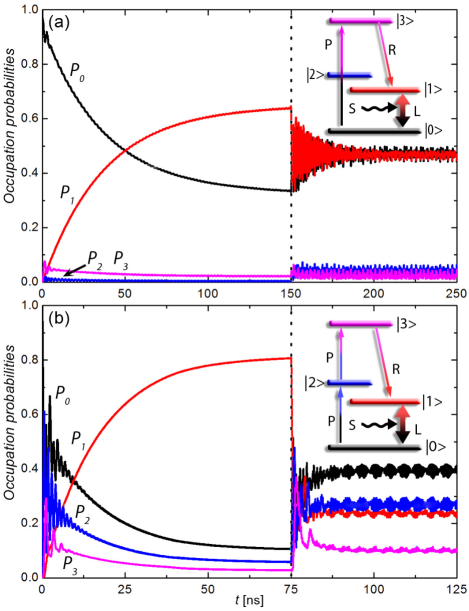
Figure 5: (Color online). Three-level lasing and stimulated transition. Time evolution of the numerically calculated occupation probabilities at biases $f_{1}=14\times 10^{-3}$ and $f_{2}=11\times 10^{-3}$ is plotted for (a) one-photon driving and (b) two-photon driving. As shown in the inset schemes, the driving and fast relaxation create the inverse population between the levels $\lvert{1}\rangle$ and $\lvert{0}\rangle$. So, these levels can be used for lasing, which we schematically mark by the double arrow. After some time delay (when the population inversion is reached) an additional periodic signal (S) $f_{\mathrm{L}}\cos\omega_{\mathrm{L}}t$ is turned on matching the operating levels, $\hbar\omega_{\mathrm{L}}=E_{1}-E_{0}$. This leads to the stimulated transition $\lvert{1}\rangle\rightarrow\lvert{0}\rangle$.

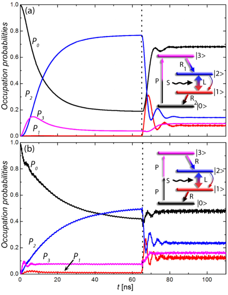
Figure 6: (Color online). Four-level lasing and stimulated transition. Time evolution of the occupation probabilities at biases $f_{1}=14\times 10^{-3}$ and $f_{2}=20\times 10^{-3}$ is plotted for (a) one-photon driving and (b) two-photon driving. The driving and fast relaxation create the inverse population between the levels $\lvert{2}\rangle$ and $\lvert{1}\rangle$. After a time delay an additional periodic signal $f_{\mathrm{L}}\cos\omega_{\mathrm{L}}t$ is turned on matching the operating levels, $\hbar\omega_{\mathrm{L}}=E_{2}-E_{1}$. This leads to the stimulated transition $\lvert{2}\rangle\rightarrow\lvert{1}\rangle$.

In Fig. 5 we consider the situation where the relevant dynamics includes three levels (for definiteness, we take $f_{1}=14\times 10^{-3}$, $f_{2}=11\times 10^{-3}$, which is marked as the square in Fig. 4). Pumping ($\lvert{0}\rangle\rightarrow\lvert{3}\rangle$) and relaxation ($\lvert{3}\rangle\rightarrow\lvert{1}\rangle$) create the population inversion between the levels $\lvert{1}\rangle\$and $\lvert{0}\rangle$. For pumping we consider two possibilities: one-photon driving, Fig. 5(a), when $\hbar\omega=E_{3}-E_{0}$, and two-photon driving, Fig. 5(b), when $2\hbar\omega=E_{3}-E_{0}$. In the latter case we have chosen the parameters (namely $f_{1}$ and $f_{2}$) so, that the two-photon excitation goes via an intermediate level $\lvert{2}\rangle$. We note here that, as was demonstrated in Ref. Ilichev10, , the multi-photon excitation in our multi-level system can be direct, as below in Fig. 6(b), or ladder-type, via an intermediate level, as in Fig. 5(b). Figure 5 was calculated for the following parameters: $\omega_{\mathrm{L}}/2\pi=13.7$ GHz ($\hbar\omega_{\mathrm{L}}=E_{1}-E_{0}$) and also (a) $\omega/2\pi=35.2$ GHz, $f_{\mathrm{ac}}=7\times 10^{-3}$, $f_{\mathrm{L}}=5\times 10^{-3}$; (b) $\omega/2\pi=17.6$ GHz, $f_{\mathrm{ac}}=2\times 10^{-3}$, $f_{\mathrm{L}}=5\times 10^{-3}$.

Next, we consider the scheme for the four-level lasing, which occurs in a similar scenario, except the changing of the levels. Then, the main relaxation transitions are $\lvert{3}\rangle\rightarrow\lvert{2}\rangle$ and $\lvert{1}\rangle\rightarrow\lvert{0}\rangle$, and now the population inversion should be created between levels $\lvert{2}\rangle$ and $\lvert{1}\rangle$. For this we take the partial biases $f_{1}=14\times 10^{-3}$, $f_{2}=20\times 10^{-3}$ (marked by the circle in Fig. 4). First, the system is pumped only with one signal either with $\hbar\omega=E_{3}-E_{0}$, Fig. 6(a), or with $2\hbar\omega=E_{3}-E_{0}$, Fig. 6(b). Such pumping together with fast relaxation ($\lvert{3}\rangle\rightarrow\lvert{2}\rangle$) creates the population inversion between the levels $\lvert{2}\rangle\$and $\lvert{1}\rangle$. Fast relaxation from lower laser level $\lvert{1}\rangle$ into the ground state $\lvert{0}\rangle$ helps creating the population inversion between the laser levels $\lvert{2}\rangle\$and $\lvert{1}\rangle$, which is the advantage of the four-level scheme.Svelto Then the second signal is applied with a frequency matching the laser operating levels ($\hbar\omega_{\mathrm{L}}=E_{2}-E_{1}$). This stimulates the transition $\lvert{2}\rangle\rightarrow\lvert{1}\rangle$, which provides the scheme for the four-level lasing. Figure 6 was calculated for the following parameters: $\omega_{\mathrm{L}}/2\pi=9$ GHz ($\hbar\omega_{\mathrm{L}}=E_{2}-E_{1}$) and also (a) $\omega/2\pi=47.4$ GHz, $f_{\mathrm{ac}}=5\times 10^{-3}$, $f_{\mathrm{L}}=3\times 10^{-3}$; (b) $\omega/2\pi=23.7$ GHz, $f_{\mathrm{ac}}=5\times 10^{-3}$, $f_{\mathrm{L}}=5\times 10^{-3}$.

In the experimental realization of the lasing schemes proposed here, the system of two qubits should be put in a quantum resonator, e.g. by coupling to a transmission line resonator, as in Ref. Astafiev07, . Then the stimulated transition between the operating states, which we have demonstrated here, will result in transmitting the energy from the qubits to the resonator as photons. For this, the energy difference between the operating levels should be adjusted to the resonator’s frequency.

V Conclusions and Discussion

We have considered the dissipative dynamics of a system of two qubits. Assuming different qubits makes some of the relaxation rates dominant. With these fast relaxation rates, population inversion can be created involving three or four levels. The four-level situation is more advantageous for lasing since the population inversion between the operating levels can be created more easily. We demonstrated that the upper level can be pumped by one- or multi-photon excitations. We also have shown that after applying additional driving, the transition between the operating levels is stimulated.

When presenting concrete results, we have considered the system of two flux superconducting qubits with the realistic parameters of Ref. Ilichev10, . For lasing in a generic two-qubit (four-level) system, our recipe is the following. The hierarchy of the relaxation times in the system is obtained by making it asymmetric, with different parameters for individual qubits. This makes transitions between the levels corresponding to a qubit with smaller tunneling amplitude $\Delta$ negligible, which creates a sort of the artificial selection rule. Based on our numerical analysis, we conclude that the optimal combination of pumping and relaxation is realized for $\Delta_{1}\gg\Delta_{2}\sim J$.

Creation of the population inversion and the stimulated transitions between the laser operating levels, demonstrated here theoretically, can be the basis for the respective experiments similar to Ref. Astafiev07, . In that work, a three-level qubit (artificial atom) was coupled to a quantum (transmission line) resonator. First, spontaneous emission from the upper operating level was demonstrated. In this way the qubit system can be used as a microwave photon source.Houck09 Then, the operating levels were driven with an additional frequency and the microwave amplification due to the stimulated emission was demonstrated. We believe that similar experiments can be done with the two-qubit system (which forms an artificial four-level molecule from two atoms/qubits). To summarize, we propose to put the two-qubit system in a quantum resonator with the frequency adjusted with the operating levels and to measure the spontaneous and stimulated emission as the increase of the transmission coefficient. Such lasing in a two-qubit system may become a new useful tool in the qubit toolbox.

- (1) For reviews see Special issue on quantum computing with superconducting qubits, Quant. Inf. Process., Vol. 8, Nos. 2-3 (2009).
- (2) S.K. Dutta et al., Phys. Rev. B 78, 104510 (2008); D.M. Berns et al., Nature 455, 51 (2008); M. Neeley et al., Science 325, 722 (2009); H. Jirari et al., Eur. Phys. Lett. 87, 28004 (2009); M.A. Sillanpää et al., Phys. Rev. Lett. 103, 193601 (2009); G. Sun et al., Appl. Phys. Lett. 94, 102502 (2009); J. Joo et al., Phys. Rev. Lett. 105, 073601 (2010); L. Du and Y. Yu, Phys. Rev. B 82, 144524 (2010).
- (3) A. Wallraff et al., Nature 431, 162 (2004); J. Hauss et al., Phys. Rev. Lett. 100, 037003 (2008); A.A. Abdumalikov et al., Phys. Rev. Lett. 104, 193601 (2010); S. Ashhab and F. Nori, Phys. Rev. A 81, 042311 (2010).
- (4) Yu.A. Pashkin et al., Nature 421, 823 (2003); J.B. Majer et al., Phys. Rev. Lett. 94, 090501 (2005); M. Grajcar et al., Phys. Rev. B 72, 020503 (2005); M. Steffen et al., Science 313, 423 (2006); A. Fay et al., Phys. Rev. Lett. 100, 187003 (2008); A. Izmalkov et al., Phys. Rev. Lett. 101, 017003 (2008); J. Li et al., Phys. Rev. B 78, 064503 (2008); L. DiCarlo et al., Nature 460, 240 (2009); F. Altomare et al., Nature Phys. 6, 777 (2010).
- (5) O. Astafiev et al., Nature 449, 588 (2007).
- (6) M. Grajcar et al., Nature Phys. 4, 612 (2008); S. André et al., Phys. Scr. T137, 014016 (2009); S. Ashhab et al., New J. Phys. 11, 023030 (2009); O.V. Zhirov and D.L. Shepelyansky, Phys. Rev. B 80, 014519 (2009); M.A. Macovei, Phys. Rev. A 81, 043411 (2010).
- (7) O. Svelto, Principles of Lasers, Plenum Press, New York (1989).
- (8) E. Il’ichev et al., Phys. Rev. B 81, 012506 (2010).
- (9) C.H. van der Wal et al., Eur. Phys. J. B 31, 111 (2003).
- (10) K. Blum, Density Matrix Theory and Applications, Plenum Press, New York–London (1981); U. Weiss, Quantum Dissipative Systems, 2nd ed., World Scientific, Singapore (1999).
- (11) Yu. Makhlin, G. Schön and A. Shnirman, Rev. Mod. Phys. 73, 357 (2001); M. Governale et al., Chem. Phys. 268, 273 (2001); M.J. Storcz and F.K. Wilhelm, Phys. Rev. A 67, 042319 (2003); M.J. Storcz, PhD thesis (2002); L. Chirolli and G. Burkard, Advances in Physics 57, 225 (2008); Y. Dubi and M. Di Ventra, Phys. Rev. A 79, 012328 (2009).
- (12) Yu-xi Liu et al., Phys. Rev. Lett. 95, 087001 (2005); J.Q. You et al., Phys. Rev. B 71, 024532 (2005); J.Q. You et al., Phys. Rev. B 75, 104516 (2007).
- (13) P.C. de Groot et al., Nature Phys. 6, 763 (2010).
- (14) E. Paladino et al., Phys. Scr. T137, 014017 (2009).
- (15) S.N. Shevchenko and E.A. Temchenko, J. Phys.: Conf. Ser. 129, 012035 (2008).
- (16) A.A. Houck et al., Nature 449, 328 (2007).