IFUM-967-FT
Parton distributions at the dawn of the LHC
Stefano Forte
Dipartimento di Fisica, Università di Milano and
INFN, Sezione di Milano,
Via Celoria 16, I-20133 Milano, Italy
Abstract
We review basic ideas and recent developments on the determination of the parton substructure of the nucleon, in view of applications to precision hadron collider physics. We review the way information on PDFs is extracted from the data exploiting QCD factorization, and discuss the current main two approaches to parton determination (Hessian and Monte Carlo) and their use in conjunction with different kinds of parton parametrization. We summarize the way different physical processes can be used to constrain different aspects of PDFs. We discuss the meaning, determination and use of parton uncertainties. We briefly summarize the current state of the art on PDFs for LHC physics.
To the memory of Wu-Ki Tung
November 2010
1 QCD in the LHC era
The theory and phenomenology of the strong interactions [1] have witnessed an impressive development in the last two decades, driven first by the availability of HERA [2] — a QCD machine — and then by the needs of present (Tevatron) and especially upcoming (LHC) hadron colliders [3]. The LHC will be looking for new physics in hadronic collisions.
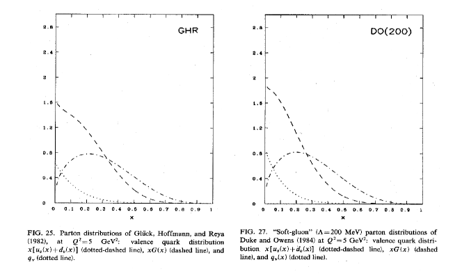
The last time this happened was back in the early eighties, when the and were discovered at the SPS collider [4] — and, of course, one may argue to which extent the and then were genuinely “new” physics. At the time, QCD was at best a semi-quantitative theory: for example, in Ref. [5] a measured cross section of nb (at GeV) was described as “in agreement with the theoretical expectation” [6] of nb. One reason why at that time a NLO calculation couldn’t be expected to agree with the data to better than 20% is that the knowledge of nucleon structure was at the time extremely sketchy: a parton set consisted of three parton distributions (valence, quark sea, and gluon), differences at the 30% level between sets would be standard, and, of course, there would be no idea on the associate uncertainty (see Fig. 1).
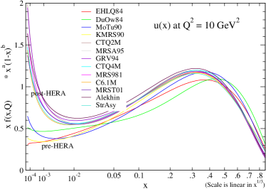
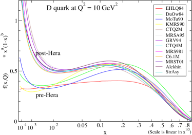
The evolution in time of parton distributions (see Fig. (2)) since then shows that it is only during the HERA age that predictions from different groups converged: this is both a consequence and a cause of the fact that perturbative QCD has now turned into a quantitative theory, which leads to predictions for hard processes with typical accuracies below 10%, and often of a few percent. Perturbative QCD today is an integral part of the Standard Model, and it is tested to an accuracy which is comparable to that of the electroweak sector: in fact, HERA has played for QCD a similar role as LEP for electroweak theory. In the last decade, theoretical and phenomenological progress has been impressive: at the LHC we can envisage quantitative control of QCD contribution to collider signal and background processes at the percent level, as will be necessary for discovery at the LHC [3].
Progress in QCD has taken place in (at least) five distinct directions, namely (listing from the bottom beam nucleons up to the final state): First, the understanding of the structure of the nucleon in terms of parton distributions has now become a quantitative science. Second, perturbative computations are being pushed to hard processes with increasingly high numbers of particles and at increasingly high orders, thanks to the development of a variety of techniques which include twistor methods, analyticity techniques, and the use of exact results from supersymmetric QCD and the AdS/CFT duality. Third, all-order resummation of perturbation theory is being extended in various kinematic regimes (small and large ) to new classes of observables (typically less inclusive), to higher logarithmic orders, and it is being accomplished using perturbative renormalization-group methods, path integral techniques, and effective field theory methods. Fourth, definitions of jet observables which are both consistent with perturbative factorization to all orders and numerically efficient have been constructed theoretically and implemented in computer interfaces. Fifth, new collinear subtraction algorithms have been developed which make the development and implementation of next-to-leading order Monte Carlo codes possible.
The lectures at the Zakopane school on which this paper is based, ambitiously entitled “QCD at the dawn of the LHC”, covered the first three of these topics: parton distributions (PDFs), perturbative computations, and resummation. Here we will concentrate on PDFs; recent good reviews of progress in perturbative computations are in Refs. [11, 12], while a comprehensive overview of resummation is unfortunately not available yet. At Zakopane, jets and Monte Carlos where discussed by other speakers; excellent recent reviews of these topics are in Refs. [13, 14] respectively.
The purpose of this overview of PDFs is both to provide an elementary introduction to the subject, and also a summary of recent developments, several of which are little known outside a small group of practitioners. Progress in this field has been largely driven by two series of HERA-LHC workshops 2004-1005 and 2006-2007, which have organized and stimulated the transfer of know-how from deep-inelastic scattering to hadron collider physics, and whose results are collected in the respective reports Refs. [15, 16]. Since 2007, the PDF4LHC working group has been formed [17] with a mandate from the CERN directorate to steer and coordinate research on PDFs for the LHC community: many of the more recent ideas discussed here were developed in the context of this working group.
This review is organized as follows. We will start with the more basic concepts, then work our way to somewhat more advanced developments. First, we will very briefly review some basic (mostly kinematic) facts on QCD factorization. We will then present the two main existing approaches (Hessian and Monte Carlo) to the determination of PDFs and the way they are used in conjunction with various forms of parton parametrization. Next, we will review standard ideas on how information on PDFs can be extracted from the data. We will then discuss in some detail the problem of PDF uncertainties — what they mean and how they are determined. In the final section we will briefly summarize the state of the art: the role of theoretical uncertainties, and the current understanding of standard candle processes at the LHC.
These lectures are dedicated to the memory of Wu-Ki Tung, who pioneered this field, pursued it for more than 30 years, and shaped much of our current understanding of it.
2 Factorization
Factorization of cross sections into hard (partonic) cross sections and universal parton distributions is the basic property of QCD which makes it predictive in the perturbative regime, and which enables a determination of parton distributions. Here we only review some basic facts which will be useful for our subsequent discussion, while referring to standard textbooks [18] and recent reviews [1] for a detailed treatment.
2.1 Electro- and hadro-production kinematics
The basic factorization for hadroproduction processes has the structure
where is the distribution of partons of type in the -th incoming hadron; is the parton-level cross section for the production of the desired (typically inclusive) final state ; the minimum value of is , with
| (2) |
the scaling variable of the hadronic process, and in the last step we defined the parton luminosity
| (3) |
The hard coefficient function is defined by viewing the parton-level cross section as a function of the hard scale and the dimensionless ratio of this scale to the center-of-mass energy of the partonic subprocess:
| (4) |
in terms of the scaling variable. At the lowest order in the strong interaction, the partonic cross section is then either zero (for partons that do not couple to the given final state at leading order), or else just a function fixed by dimensional analysis times a Dirac delta, and the hard coefficient function is thus defined as
| (5) |
where is a matrix with non-vanishing entries only between quark and antiquark states, which will be discussed explicitly in Sect. 2.2 below (see in particular Eqs. (18-19). For example, for virtual photon (Drell-Yan) production is nonzero when is a pair of a quark and an antiquark of the same flavour, and in such case .
The factorized result Eq. (2.1) holds both for inclusive cross sections and for rapidity distributions.:
| (6) |
where the hadronic cross section is differential with respect to the rapidity of the final state , while the partonic cross section is differential in partonic rapidity
| (7) |
the effect of parton emission from the incoming hadrons is to perform a Lorentz boost from the hadronic center-of-mass frame to a frame in which the energy of each of the two incoming hadrons are rescaled by and respectively. The lower limit of integration is then fixed by requiring that the rapidity of the incoming partons be at least sufficient to yield the observed final state rapidity:
| (8) |
At leading order, the two partons couple directly to the final state so and
| (9) |
Equation (2.1) is to be contrasted with the standard factorization for the deep-inelastic structure functions :
| (10) |
Here in the argument of the structure function is the standard Bjorken variable and the hard coefficient function is the structure function computed with an incoming parton and is the distribution of the -th parton in the only incoming hadron. Also in this case at lowest it is either zero (for incoming gluons) or a constant (an electroweak charge) times a Dirac delta.
Note that the structure functions are related to the cross section which is actually measured in lepton-hadron scattering by
| (11) |
for neutral-current charged lepton DIS, where the longitudinal structure function is defined as
| (12) |
and
| (13) |
in terms of the electron momentum fraction
| (14) |
(not to be confused with the partonic rapidity Eq. (7)) where and are respectively the incoming proton and lepton momenta, is the virtual photon momentum () and in the last step, which holds neglecting the proton mass, is the center-of-mass energy of the lepton-proton collision. Similar expressions hold for charged-current charged and neutral lepton scattering.
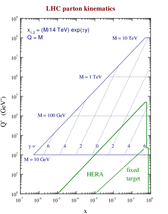
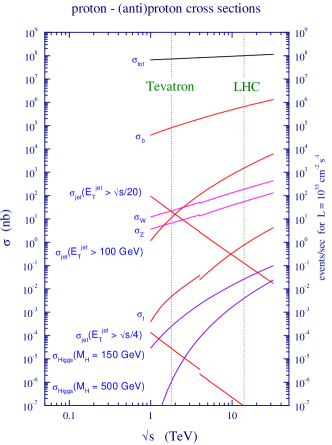
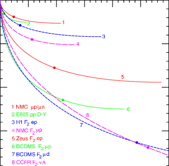
The set of values of over which the PDF is probed is of course the same in the hadro- and leptoproduction cases, and it ranges from the scaling variable of the hadronic process to one: in Eq. (10), and in Eq. (2.1). The kinematic region which is typical of of collider (HERA) or fixed-target DIS experiments is compared in Fig. 3 to that of LHC processes, whose typical cross sections are also shown.
There is an important kinematic difference when comparing the hadronic and deep-inelastic factorization formulae, Eqs. (2.1) and (10) respectively. This is related to the fact that the leading order coefficient function is proportional to a Dirac delta. For DIS, this implies that at leading order, the value of the structure function at given determines the quark distributions at the same value of , and it is only at next-to-leading order, where the coefficient function has a nontrivial dependence on , that the PDF is probed for all values . But for hadronic processes, because there are two partons in the initial state, even at leading order, for inclusive cross sections the delta kills one but not both of the convolution integrals in Eq. (2.1), so all values are probed. However, for rapidity distributions because of the further kinematic constraint Eq. (9) the leading order kinematics is also fixed, and for given and the momentum fractions of both partons are fixed.
2.2 Constraints on PDFs
The kinematics of the factorized expressions Eqs. (2.1) and (10) immediately implies that, as discussed in Sect. 2.1, at leading order deep-inelastic structure functions and rapidity distributions provide a direct handle on individual quark and antiquark PDFs (DIS), or pairs of PDFs (Drell-Yan). It is possible to understand what is dominantly measured by each individual process by looking at the leading order expressions, bearing in mind that, of course, beyond leading order all other contributions turn on (and that NLO corrections can be quite large, in fact of the same order of magnitude as the LO for Drell-Yan).
The leading order contributions to the DIS structure functions and are the following (at leading order ):
|
(15) |
where and denotes neutral or charged current scattering and we have lumped together the contributions coming from exchange and from interference, with couplings given by
| (16) | |||||
| (17) |
in terms of the electroweak couplings of quarks and leptons listed in Table 1 and the propagator correction .
| fermions | |||
| u,c,t | +2/3 | +1/2 | |
| d,s,b | -1/3 | -1/2 | |
| 0 | +1/2 | +1/2 | |
| e, | -1 | -1/2 |
The leading order contribution to Drell-Yan is given by
|
|
(18) |
in terms of the differential leading order parton luminosity
| (19) |
and the CKM matrix elements , with given by Eq. (8). This shows explicitly that, as already mentioned, for a rapidity distribution the leading order parton kinematics (i.e. the values of ) is completely fixed by the hadronic kinematics (i.e. the values of and ).
Note that while at a collider (or when a beam collides with a fixed target) such as the LHC it makes no difference whether the incoming quark and antiquark come from either of the initial-state hadrons, at a collider such as the Tevatron (or when a beam collides with a deuterium fixed target) there are two different contributions, according to whether each of the incoming partons is extracted from either of the initial-state hadrons.
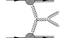
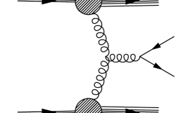
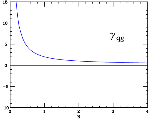
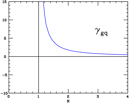
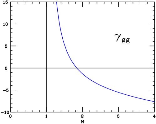
Leading-order information on the gluon can be extracted from jet production (see Fig. 4), or from scaling violations, as measured for instance by the dependence of deep-inelastic structure functions. The latter are coupled to the gluon even at leading order through the singlet QCD evolution equations, which in terms of Mellin moments
| (20) |
of parton distributions take the form
| (21) | |||||
| (22) |
where the singlet combination of quark distributions is defined as
| (23) |
and the remaining nonsinglet combinations can be taken as any linearly independent set of differences of quark and antiquark distributions, which all evolve according to individual, decoupled equations.
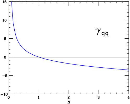
The leading order anomalous dimensions are shown in Fig. 5, while at leading order all nonsinglet are equal to each other and are also equal to . The qualitative behaviour of perturbative evolution is then deduced recalling that Mellin transformation maps the large (small ) () region into the large (small) ( region. A first relevant feature is that as the scale increases all PDFs decrease at large and increase at small . A second important feature is that because the gluon has the rightmost singularity at small it drives small scaling violations, and thus in particular at sufficiently small and large all PDFs have the same shape, driven by the gluon. Finally, the evolution of the gluon (driven by ) is strongest at either large or small but its coupling to the quark (driven by ) is only large at small , so it is only at not too large that scaling violations provide leading constraints on the gluon.
Finally, it is important to note that constraints on PDFs come from their cross-talk imposed by sum rules: specifically the conservation of baryon number
| (24) |
and the conservation of total energy-momentum
| (25) |
Clearly, these sum rules provide constraints on the behaviour of parton distributions even in the region where there are no data.
3 Statistics
A determination of parton distributions is a determination of at least seven independent functions: three light quark and antiquark distributions and the gluon at some initial scale, from which PDFs at all other scales can be obtained solving evolution equations. More functions must be determined if one wishes to keep open the possibility [19] that heavy quarks PDFs are at least in part of “intrinsic” nonperturbative origin, rather than being determined radiatively from gluons by QCD evolution. A determination of PDFs with uncertainties thus involves determining a probability distribution in a space of several independent functions. Because experimental data used for this determination will always be finite in number, this is in principle an ill-posed (or unsolvable) problem.
The time-honored [20, 21] method to make this problem tractable is to assume a specific functional form for parton distributions, which projects the infinite dimensional problem onto a finite-dimensional parameter space. This method is justified because PDFs are expected to be smooth functions of the scaling variable . Because , a representation of these functions with finite accuracy must be possible on a finite basis of functions: hence, a representation of PDFs must be possible in terms of a finite number of parameters. The problem is then reduced to the choice of an optimal parametrization, namely, one that for given accuracy minimizes the number of parameters without introducing a bias. We will discuss below two such parametrizations.
Whatever the parametrization, determining a set of PDFs involves computing a number of physical processes with a given set of input PDFs, and extremizing a suitable figure of merit, such as a or likelihood function in order to determine a best-fit set of PDFs. Existing sets of parton distributions which are made available for the computation of LHC processes through standard interfaces are determined and delivered following two main strategies: a “Hessian” approach, in which the best-fit result is given in the form of an optimal set of parameters and an error matrix centered on this optimal fit to compute uncertainties, and a Monte Carlo approach, in which the best fit is determined from the Monte Carlo sample by averaging and uncertainties are obtained as variances of the sample.
It turns out that available Hessian PDF sets are mostly based on a “standard” parametrization, inspired by various QCD arguments. On the other hand, the only available full Monte Carlo PDF set is based on a rather different form of parametrization, which adopts neural networks as interpolating functions in an attempt to reduce the bias related to the choice of functional form [22]. However, Monte Carlo studies based on other standard [23] and non-standard [24] parametrizations have also been presented.
Here we will summarize the main features of both the Hessian and Monte Carlo approach, and in each case also discuss the parton parametrization which is most commonly used with each approach, and the way the best fit is determined in each case — which in turn requires a peculiar algorithm within the neural network approach.
3.1 Hessian uncertainties and the “standard” approach
The standard approach to PDF determination is based on assuming for PDFs at some reference scale a functional form inspired by counting rules [25], which suggest that PDFs should behave as , and Regge theory, which suggest [26] that they should behave as . Note that these limiting behaviours are necessarily approximate, because even if they hold at some scale, at any other scale perturbative evolution will correct them by logarithmic terms which behave as as and as as . Therefore, even if counting rules and Regge theory actually provide predictions for the values of the exponents and respectively (for given parton and parent hadron), they are taken as free fit parameters.
Based on this, typically PDFs are assumed to have the form
| (26) |
where tends to a constant for both and . For instance, the CTEQ/TEA collaboration assumes generally [27, 28]
| (27) |
with different parameters for each PDF, but some parameters fixed or set to zero for some PDFs — for example, parameters and are nonzero only for the gluon distribution. Other groups assume that is a polynomial in or in : for instance HERAPDF [29] assumes .
Different choices are possible for the set of linearly independent combinations of PDFs for which the parametrization Eq. (26) is adopted, and for the total number of free parameters to be used. For instance CTEQ/CT parametrizes the “valence” light combinations , , the antiquark distributions and , the two strangeness combinations (but in the CTEQ6.6 [27] and CT10 [28] fits it is assumed that ) and the gluon, with 22 (CTEQ6.6) or 26 (CT10) free parameters; MSTW08 [30] parametrizes also , , and the gluon, and then the two combinations with a total of 28 parameters, and so forth.
Given a parametrization of PDFs, the problem is reduced to that of determining best fit values and uncertainty ranges for the parameters. In a Hessian approach, this is done by minimizing a figure of merit such as
| (28) |
where the sum runs over all data points, are experimental data with experimental covariance matrix (including all correlated and uncorrelated statistical and systematic uncertainties), are theoretical predictions which are obtained by evolving the starting PDFs at any scale using the evolution equations Eq. (22), and then folding the result with known partonic cross sections according to the factorization theorems Eqs. (2.1,6,10), and denotes the full set of parameters on which the PDFs at scale depend, which we may view as a vector in parameter space (which is 26-dimensional for CT10, and so on). The thus is a function of the through the predictions .
Note that the Eq. (28) is normalized to the number of data points: this is conventionally done in order to allow for approximate comparisons of fit quality between fits with different numbers of data points; in practice, this is likely to be close to the per degree of freedom because typical datasets include thousands of data, while the total number of parameters needed to describe accurately all PDFs with functional forms like Eq. (26), though of course unknown, is likely to be rather lower than a hundred. For the sake of future discussions it is convenient to also introduce an unnormalized
| (29) |
It is important to note that there are subtleties in the definition of the , which may make the comparison of values from different groups only qualitatively significant, because slightly different definitions are used. The main subtlety is related to the inclusion of normalization uncertainties, which cannot be simply introduced in the covariance matrix, as this would bias the fit [31]: a full unbiased solution [32] requires an iterative construction of the covariance matrix, but other approximate solutions are also adopted.
Once the is defined, for given data is a function of the PDF parameters through the predictions which in turn depend on the PDFs. Hence, the best fit set of parameters can be identified with the absolute minimum of the in parameter space. Furthermore, the variance of any observable which depends on parameters (such as a physical cross section, or indeed the PDFs themselves), if we assume linear error propagation , is given by
| (30) |
Here is the covariance matrix of the parameters which, in turn, assuming that the is a quadratic function of the parameters in the vicinity of the minimum, is given by (see e.g. [33, 34])
| (31) |
i.e. it is the (Hessian) matrix of second derivatives of the unnormalized Eq. (29), evaluated at its minimum.
The Hessian method for the determination of uncertainties thus in particular implies that the one- (i.e. 68% confidence level) for the parameters themselves is the ellipsoid in parameter space which is fixed by the condition . As we will discuss in Sect. 5.1 in practice this argument may have to be modified in realistic cases, in order to account for various effects (such as incorrect estimation of the covariance matrix of the data).
However, for the time being let us stick to the textbook argument, and make a couple of observations on it. The first observation is that we are always free to adjust the parametrization in such a way that all eigenvalues of the Hessian matrix are equal to one, by simply diagonalizing the matrix and rescaling the eigenvectors by the eigenvalues, i.e. by looking for new parameters such that
| (32) |
which immediately implies that
| (33) |
where the gradient is computed with respect to . Equation (33) has the immediate interesting consequence that the total contribution to the uncertainty due to two different sources, being the length of a vector, is simply found by adding the components i.e. the different uncertainties in quadrature (even when the two uncertainties are correlated). This has been emphasized recently in Ref. [35], where it is shown explicitly that, contrary to what one may naively think, the total uncertainty due to PDF parameters and some other parameter (such as the value of the strong coupling constant) is simply found adding the two uncertainties in quadrature.
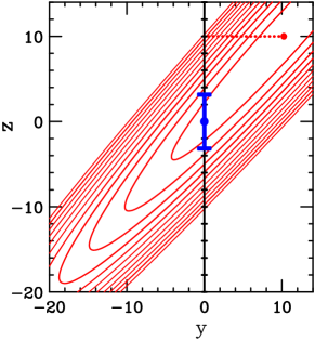
The second comment has to do with the fact that the one- interval in parameter space corresponds to the contour about the minimum. This is identical to the statement that the Hessian Eq. (31) is the covariance matrix in parameter space. This simple fact is sometimes source of confusion because it seems to contradict the observation that the standard deviation of the (unnormalized) distribution with degrees of freedom is : in fact, sometimes (see e.g. [36]) it is incorrectly stated that one- contours correspond to . However, the contradiction is only apparent: sets a hypothesis-testing criterion [37], namely, it gives the size of fluctuations of upon repetition of the experiment, and thus the range of values away from the mean which are acceptable for a given theory (experiment). One the other hand provides a parameter-fitting criterion [37]: it gives the range of parameter values which are compatible at one sigma for a given experimental result (and theory).

A simple example may help in understanding the distinction. Consider the case of a simple linear fit, in which one has a set of data which are expected to satisfy a linear law , with unknown intercept that one wishes to determine by fitting to data (see Fig. 6). Define the deviation between the -th data point and the linear prediction . If are gaussianly distributed with standard deviation about their true values, then clearly the average square deviation . This is the “hypothesis testing” fluctuation range of the . However, the best-fit intercept is just the average deviation , and the square uncertainty on it is : so the “parameter fitting” range for is indeed by a factor smaller than the expected total square fluctuation, because the best-fit value is determined as a mean, whose square fluctuation is by a factor smaller than the fluctuation of the individual data.
3.2 Monte Carlo uncertainties and the NNPDF approach
A Monte Carlo approach differs from the Hessian approach in the way the uncertainty on the observable is determined in terms of the uncertainties in parameter space: the distinction Hessian vs. Monte Carlo thus has to do only with the way uncertainties are propagated from parameters to observables. However, the Monte Carlo way of propagating uncertainties is especially convenient when used together with a parametrization whose functional form is less manageable, for instance because the number of parameters is particularly large, or because the functional form is less simple than that of Eq. (26), or, more, in general, whenever linear error propagation and the quadratic approximation to the in parameter space are not advisable, for reasons of principle or of practice. Therefore, we will first discuss the distinction between Hessian and Monte Carlo per se, then turn a brief review of the way a Monte Carlo approach has been used by the NNPDF group together with a choice of basic underlying functional form for PDFs which differs from that of Eq. (26), and finally address some issues related to the determination of the best fit PDFs when such functional forms are adopted.
3.2.1 Monte Carlo uncertainties
Whereas in a Hessian approach parameters are assumed to be gaussianly distributed with covariance matrix given by the Hessian Eq. (31), in a Monte Carlo approach the probability distribution in parameter space is given by assigning a Monte Carlo sample of replicas of the total parameter set. For example, if one uses the parametrization Eq. (26) one would then simply give a list of replica copies of the vector of parameters . Any observable is then computed by repeating its determination times, each time using a different parameter replica: the central value for is the average of these results, the standard deviation is the variance, and in fact any moment of the probability distribution can be determined from the sample of values of thus obtained.
Of course, this begs the question of how the distribution of parameter values, i.e. the distribution of parameter replicas is determined in the first place. In fact, this may look like a hopeless task: let’s say that for each parameter the probability distribution in parameter space is given for each parameter as a histogram with three bins, one corresponding to the one- region about the central value of the given parameter, and two for the two outer regions. Then, for parameters the total number of bins is equal to with parameters. Hence it looks like the total number of replicas must be hopelessly large in order to have sufficient statistics. This, however, is not necessarily the case, because it may well turn out that most of the bins are actually empty. To understand this, recall the Hessian computation of the uncertainty on Eq. (33): it is clear that in order to determine the uncertainty on , it is sufficient to know the distribution in parameter space along the direction of . Hence, for this specific observable only one parameter is relevant. Even if one wants to determine the uncertainty on observables which probe any direction in parameter space, for any reasonably smooth function the number of bins which is needed in order to get an accurate representation of the probability distribution is likely to be much smaller than . This then again raises the question of how one should sample the replica distribution in parameter space.
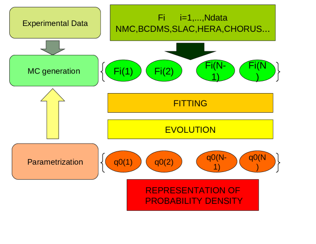
The answer is found by noting that the maximum likelihood method gives a way of mapping the probability distribution in data space onto the probability distribution in parameter space. Namely, assume one has data with covariance matrix . Then, generate data replicas , with . For each value of , i.e. for each replica, the whole set of data is replicated, in such a way that if one takes the average over the replicas of the -th data point, then in the limit this average tends to the original data value ; if one computes the variance of these values in the same limit it tends to to the the standard deviation of the data; and if one computes the covariance of the -th and -th data replicas it tends to the covariance matrix element . Now, for each data replica, determine a best-fit parameter vector by minimizing the Eq. (28), but of the fit to the replica data , rather than the original data. We end up with a Monte Carlo set of best-fit parameter vectors : again, the average over these vectors gives us the best-fit parameters , and the covariance of the -th and -th components of the parameter vector gives us the covariance matrix . In fact, it is easy to check (see e.g. [32]) that for gaussianly distributed data the results coincides with the Hessian covariance matrix Eq. (31). We will see an explicit numerical check of this equivalence in Fig. 24 below.
The procedure is summarized in Fig. 7: one starts with experimental data (denoted as in the Figure), generates data replicas (denoted as ) and fits a set of PDFs to each data replica (denoted as ). The PDFs can be parametrized in any desired way at some reference scale, and they are fitted to the data replicas in the way discussed in Sect. 3.1, namely by evolving them to the scale of the data, using them to compute observables, and minimizing the of the comparison to the data with respect to the parameters.
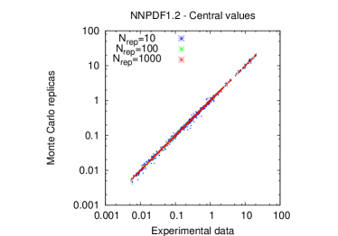
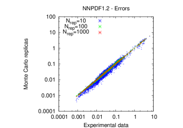
But then, the problem of constructing an adequate sampling of parameter space has been reduced to that of constructing an adequate Monte Carlo representation of the original data: i.e. the space of parameters is sampled in a way which is determined by the distribution of the data (“importance sampling”). Whether a given set of replicas provides an accurate enough representation of the data is then something that may be checked explicitly for a given sample, by comparing means, variances and covariances from the sample with the desired features of the data. For a typical set of data used in a parton fit the numbers of replicas required turn out to be surprisingly small: for instance, in Fig. 8 we show a scatter plot of the averages vs. central values and variances vs. standard deviations for the set of data points included in the NNPDF1.2 [38] parton fit, computed using Monte Carlo Replicas. It is clear that the scatter plot deviates by just a few percent from a straight line already for for central values, and for ; replicas turn out to be only necessary in order to get percent accuracy on correlation coefficients.
It should finally be mentioned that within a Monte Carlo approach it is possible to sidestep the problem of choosing an adequate parametrization by using Bayesian inference [39]. Namely, one starts from some prior Monte Carlo representation of the probability distribution based on some initial subset of data, or even on assumptions. Then, the initial Monte Carlo set is updated by including the information contained in new data through Bayes’ theorem. Without entering into details, it is clear that this can be done by changing the distribution of replicas: more or less copies are taken for those replicas which agree or respectively do not agree with the new data, in a way which is specified by Bayes’ theorem. To the extent that results do not depend too much on the choice of prior, which is often the case if the information used through Bayes’ theorem is sufficiently abundant, final results are then free of bias. Whereas the construction of a parton set fully based on this method has so far not been completed, preliminary results have been presented [40] on the inclusion of new data in an existing Monte Carlo fit using this methodology.
3.2.2 Neural Network parametrization and cross-validation
The Monte Carlo approach has been recently used for the determination of a PDF set in conjunction with the use of neural networks as a parton parametrization. Neural networks are just another functional form. In analogy to polynomial forms, they have the feature that any function (with suitable assumptions of continuity) may be fitted in the limit of infinite number of parameters; unlike polynomial forms they are nonlinear, and they are “unbiased” in that a finite-dimensional truncation of the neural network parametrization is adequate to fit a very wide class of functions (for instance, both periodic and non periodic) without the need to adjust the form of the parametrization to the desired problem.
A very simple example of neural network is the function
| (34) |
where and are free parameters. This is a neural network, parametrized by six free parameters: 1-2-1 refers to the way the neural network is constructed, by iterating recursively the response function on nodes arranged in layers which feed forward to the next layer, with the first (last) layer containing the input (output) variables.
In Refs. [38]-[41] PDFs are parametrized using 2-5-3-1 neural networks, with 37 free parameters (the input has two variables because and are treated as two independent inputs, thereby increasing the redundancy of the parametrization). The six light flavours and antiflavours are parametrized and the gluon are parametrized in this way, so that the total number of parameters is , thus rather larger than the typical numbers used when dealing with parametrizations of the form Eq. (26). Such a large number of parameters clearly reduces considerably the risk of a parametrization bias, but it poses the problem that if the best fit is determined as the absolute minimum of the one may end up fitting data fluctuations, which is clearly not desirable. Even if these fluctuations average out when averaging over Monte Carlo replicas this would be a very inefficient way of proceeding.
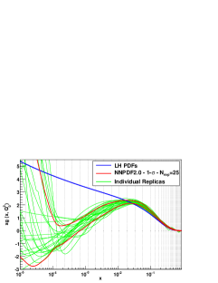
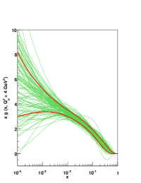
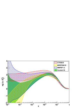
The advantage of a neural network parametrization can be understood from Fig. 9, where a gluon distribution determined using neural networks is compared to the simplest version of parametrization Eq. (26), and also to a very flexible parametrization based on orthogonal polynomials. The neural network gluon distribution shown in Fig. 9 corresponds to replicas from the Monte Carlo set of Ref. [41], and it is displayed along with the average and one- contour computed from the set. On the same plot a parametrization of the form Eq. (26) is also shown, with typical values of the parameters and , and with . It is compared to a set of Monte Carlo replicas of the gluon which were constructed in Ref. [24] by expanding the gluon distribution on a basis of 15 independent Chebyshev polynomials, while also imposing an increasing penalty to fits with large arc-length (and thus more oscillations). The fits based on orthogonal polynomials display large uncontrolled oscillations which are only tamed by appropriately tuning the length penalty. The fits based on neural networks, despite having a number of free parameters which is more than double than those using orthogonal polynomials, do not display a similarly unstable behaviour, even though they do show considerable flexibility, and in fact the ensuing one- band, though accounting well with its width for the functional freedom is actually quite stable.
The best fit is instead determined using a cross-validation method (see Fig. 10). Namely, the data are randomly divided into a training and a validation sample. The is computed both for the data in the training sample and those in the validation sample. Only the training is minimized, but the validation is also monitored as the minimization proceeds. The best fit is defined as the point at which the validation stops improving even though the training may keep improving: this is the point at which one is starting to fit the statistical noise of the training sample. In order to ensure lack of bias, the partitioning of the data is done randomly in a different way for each data replica. Also, in practice, in order to minimize the effect of random fluctuations in the data (or of the minimization algorithm) the stopping criterion must be imposed after a suitable averaging, such as for instance the moving average of values of the found in the last iterations of the minimization algorithm.
4 From data to PDFs
Once a parton parametrization and a methodology have been chosen, the determination of a PDF set relies on the choice of a set of physical observables. The problem is that, even after projecting the problem on a finite-dimensional parameter space, we must still determine seven independent PDFs, which means that we need seven linearly independent pieces of information at fixed scale for each value of . For instance, a determination of deep-inelastic structure functions and for charged-current deep-inelastic scattering provides, according to Eq. (15) four independent linear combinations of quark distributions (if can be distinguished), with two more linear combinations provided by neutral current structure functions. All individual light quark and antiquark flavours then can be determined by linear combination. This situation would be realistic at a neutrino factory with both neutrino and antineutrino beams and the possibility of identifying the charge of the final state lepton on an event-by-event basis [42, 43].
Unfortunately, this theoretically and phenomenologically very clean option is at best far in the future, so at present the information on individual PDFs can only be achieved by combining information from different processes into so-called “global” fits. The idea is that, even though each electroproduction or hadroproduction observable depends on all PDFs through the factorization formulae Eqs. (2.1,10), inclusion of specific processes or combination of processes may give a specific handle on individual PDFs or combinations of PDFs on which it depends most strongly (typically, through its leading order form). We will now review one at a time each of these individual handles on PDF, then briefly discuss how they are combined in modern more or less global fits.
4.1 Isospin singlet and triplet
Neutral current deep-inelastic (DIS) structure function data only provide a determination of the charge-conjugation even combination of quarks and antiquarks, for each quark flavor . Specifically, photon DIS data only determine the fixed combination in which each flavor is weighted by the square of the electric charge, see Eq. (15). However, one may separate off the isospin triplet and singlet components by considering DIS on both proton and deuteron targets, assuming that the deuterium structure function is simply the incoherent sum of the proton and neutron ones (up to small nuclear corrections which can be accounted for through models, such as that of Ref. [44]), and then using isospin symmetry to relate the quark and antiquark distributions of the proton and neutron:
| (35) |
One then has
| (36) |
so that the difference of proton and deuteron structure functions provides a leading-order handle on the isospin triplet combination
| (37) |
Note that even beyond leading order only depends on , which can thus be determined without further assumptions: a theoretically very clean, though necessarily not especially accurate determination [45].
4.2 Light quarks and antiquarks
Modern DIS data are available over a wide range of values of , extending well into the region where the CC contributions are sizable: in fact HERA-I data are available both for CC and NC scattering, both with electron and positron beams. Unfortunately, collider data only provide a fixed combination Eq. (11) of the structure functions and , because for given and Eq. (11) implies that can be varied only by changing the center-of-mass energy of the hadron-lepton collision. Hence, HERA data only provide three independent combinations of structure functions and thus of parton distributions (NC and CC with positively or negatively charged leptons). However, a fourth combination is provided because the dependence of the and contributions to NC scattering is different (see Eq. (17). It follows that the very precise HERA data can determine four independent linear combinations of PDFs, which can be chosen as the two lightest flavours and antiflavours, with strangeness then determined by assumption.
Even without a neutrino factory, data on neutrino deep-inelastic scattering are available, but typically on approximately isoscalar nuclear targets. Because the energy of the neutrino beam typically has a (more or less broad) spectrum, the value of Eq. (14) is not fixed, and the contributions of and to the cross section can be disentangled. On an isoscalar target at leading order
| (38) |
so neutrino data provide an accurate handle on the total valence component
| (39) |
A more direct determination of the light flavour decomposition can be obtained by exploiting the fact that the Drell-Yan cross section probes various parton combinations, which can be selected by looking at different final states. In particular one can notice [46] that for neutral-current Drell-Yan if both data on proton and neutron (or deuteron) targets are available, using isospin Eq. (35) one gets at leading order
| (40) |
where we have omitted the dependence on the kinematic variables, which at leading order is as in Eq. (18). As discussed there, if the rapidity distribution is measured, the leading order partonic kinematic is completely fixed: for given and only partons with , given by Eq. (8) contribute. Here “heavier quarks” denote strange and heavier flavours, which give a smaller contribution at least in the region of in which most of the contribution to the sum rule integrals Eq. (25,25) is concentrated.

In particular, because of the sum rule Eq. (24), in the the region which gives the dominant contribution to the integral (the “valence” region ) the up distribution is roughly twice as large as the down distribution (assuming ) so the first term in both the numerator and the denominator of Eq. (40) gives the dominant contribution, and the ratio reduces to . Hence this particular combination of cross sections provides a sensitive probe of the ratio: indeed, it has been used to provide first evidence that this ratio, though of order one, deviates from unity [47, 48].
In the charged current case, one may exploit the fact that using charge-conjugation symmetry to relate the and PDFs
| (41) |
at leading order one gets
| (42) |
where heavy quarks denotes charm and heavier flavours. In writing Eq. (42) we have assumed that cross sections are differential in rapidity. If the kinematics is chosen in such such a way that are in the “valence” region, in which quark distributions are sizably larger than antiquark ones, the ratio Eq. (42) is mostly sensitive to the light quark ratio [49, 50] and indeed it has been used to provide the first accurate determinations of it [51].
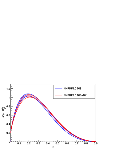
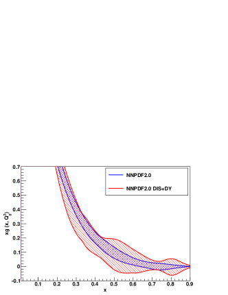
The sizable impact of Drell-Yan data on a PDF fit is demonstrated in Fig. 11, where we compare the value and uncertainty of PDF combinations which are sensitive to the light flavour decomposition before and after inclusion of Drell-Yan data in a DIS fit, namely the total valence Eq. (39) and the light sea asymmetry
| (43) |
The DIS fit includes both the fixed-target proton and neutron data (which thus determine well the isotriplet component and give a handle on the singlet-triplet separation), the precise HERA data (which give a handle on each individual light flavour and antiflavour), and several neutrino data (which give a handle on the total valence component). The Drell-Yan data included contain both proton and deuteron fixed target production data, and and production. It is apparent that the accuracy on the valence, which is already quite good in the DIS-only fit, is reduced by a large factor by the inclusion of Drell-Yan data, and the effect is even more impressive on the light antiquark asymmetry which, despite the accuracy of the HERA data, is only determined with large uncertainties by DIS data.
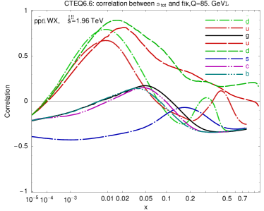
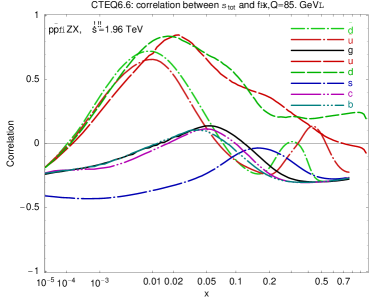
The strong impact of and production data can be seen quantitatively by computing the correlation coefficient between the and cross section and individual parton distributions, which can be computed both in a Hessian approach using standard error propagation, or in a Monte Carlo approach from the covariance of the cross section and the parton distribution over the Monte Carlo sample. Results obtained in the Hessian approach using CTEQ6.6 [27] are shown in Fig 12: correlations are quite large, even though results shown here are obtained using the total cross section, which is a much less sensitive probe of PDFs than the rapidity distributions discussed above.
4.3 Strangeness
The determination of strangeness is nontrivial because, of course, it has the same electroweak couplings as the down distribution, while it is typically smaller than it (except at small where all PDFs are the same size, as discussed in Sect. 2.2). The only way of determining it accurately from deep-inelastic scattering data is to include semi-inclusive information. A simple way of doing this is to use data for neutrino deep-inelastic charm production (known as dimuon production, because charm is tagged by the muon from its decay together with the muon due to the charged current neutrino interaction). At leading order the structure functions are then just
| (44) |
so up to CKM suppressed terms they measure strangeness directly.
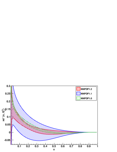
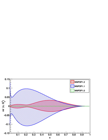
In Fig. 13 the behaviour upon inclusion of dimuon data of a fit to a set of DIS data which includes both neutrino and HERA data is shown: it is clear that before inclusion of the dimuon data the fit (NNPDF1.1 [52]) cannot determine either of the two strange combinations
| (45) |
but after their inclusion it determines both, though with limited accuracy due to the limited accuracy and kinematic coverage of the available dimuon data. In this plot, we also show the result one obtains for strangeness if one simply assumes it to be proportional to the light quark sea, i.e. if by assumption one sets and . This is often done in PDF determinations based on DIS data only: the result is then misleadingly accurate. This comparison should thus be taken as a warning that, when using PDF sets in which some PDFs are fixed by assumption, some uncertainties may be significantly underestimated.
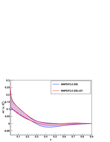
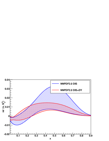
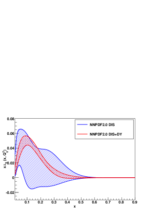
Of course the Drell-Yan data discussed above also constrain strangeness. Specifically, the cross section ratio Eq. (42) receives a contribution from strange and charm quarks which, up to CKM matrix elements, is identical to the contribution from down and up quarks respectively. Well above charm threshold this contribution is sizable, so comparing Drell-Yan data above and below charm threshold potentially leads to a rather accurate determination of strangeness. Indeed, in Fig. 14 we show the impact of including Drell-Yan data in a fit with DIS data only (same pair of fits already shown in Fig. 11). The DIS dataset contains dimuon data, and it is similar to the dataset on which the fit of Fig. 13 is based, from which it mostly differs because of improvements in the HERA data and in fit methodology; however, the Drell-Yan data have a visible impact on the total strangeness , and lead to a very striking improvement in the determination of the strangeness asymmetry .
4.4 Gluons
The determination of the gluon distribution is nontrivial because the gluon does not couple to electroweak final states. It does, however, mix at leading order through perturbative evolution: so, even using parton-model (i.e. O()) expressions for cross sections and structure functions, the gluon does determine their scale dependence. Indeed
| (46) |
where by we denote the Mellin moments Eq. (20) of the singlet component (defined as in Eq. (23)) of the structure function.
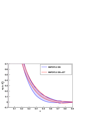
It follows that the gluon is mostly determined by scaling violations, or by its coupling to strongly–interacting final-states, i.e. jets. The main shortcoming of the determination from scaling violations is that, as already pointed out in Sect. 2.2, the gluon only couples strongly to other PDFs for sufficiently small : for instance, Fig. 5 shows clearly that for the term rapidly becomes negligible in comparison to the term. On the other hand, the gluon distribution is expected to be quite small at large , and, as also discussed in Sect. 2.2, to further shift towards smaller as the scale increases. Hence, the large gluon is likely to be small and affected by large uncertainties, which can only be reduced by looking at hadronic (jet) final states.
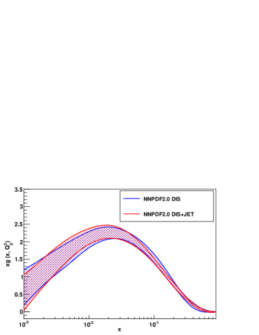
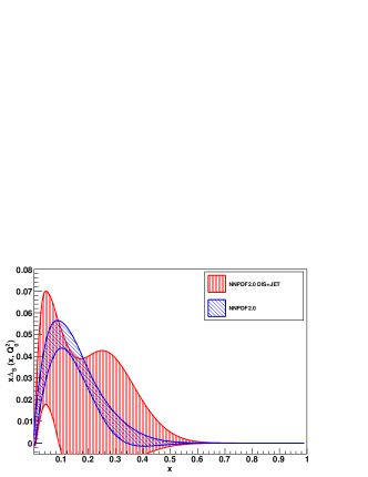
Indeed, in Fig. 15 we show the effect of the inclusion of jet data in a PDF fit based on DIS data. At small there is essentially no effect: scaling violations are sufficient to determine the gluon quite accurately. At large , even though the determination of the gluon from scaling violations is reasonably accurate, its accuracy is still quite significantly improved by the inclusion of jet data. A feature of this plot which is worth noting is the beautiful consistency of these two determinations. This is an extremely strong consistency check for the perturbative QCD framework: the gluon determined from scaling violation and evolved up to the much higher jet scale is in perfect agreement with the jet data, and indeed the best accuracy is obtained combining the two determinations.
4.5 Global fits
It is clear that the wider the number of different processes, the greater the amount of information which is being used in the determination of PDFs. The price to pay for this, as we will discuss in Sect. 5, is that the determination of PDFs and especially their uncertainties from diverse and possibly inconsistent data might be nontrivial — at the very least, it is going to be computationally intensive. Current global fits use all the processed discussed so far in order to control as much as possible different aspects of PDFs.
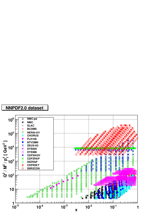
The dataset used in one such fit (NNPDF2.0 [41]) is shown in Fig. 16. Different data in this set constrain different aspects of PDFs, along the lines of the preceding discussion, in a way which, referring to this specific dataset, can be summarized as follows:
- •
-
•
an accurate determination of the behaviour of the gluon and quark at small (where it is dominated by the singlet) and by individual light flavours at medium (where CC and NC data play a role in separating individual flavours) is found from the very precise HERA CC and NC data denoted in the plot as HERAI-AV [58], which were obtained by combining the ZEUS and H1 data from the HERA-I run. More recent HERA-II ZEUS NC [59] and CC [60] data (ZEUS-H2) are also used.
- •
- •
-
•
the total valence component is constrained by the neutrino inclusive DIS data, denoted as CHORUS [68] in the plot;
- •
- •
Other global fits may differ in some detail, such as the specific choice of experiments or the addition or subtraction of some set of data, but are mostly based on datasets constructed on the basis of a similar logic. Smaller datasets, typically a subset of the above, are also considered.
Future improvements on some of these processes, in particular Drell-Yan (including and ) production and jet production will certainly come from the LHC, both because of the higher available center-of-mass energy (compare Fig. 3), and because of the higher statistics which will be accumulated once higher or design luminosity are reached. Some other processes which are likely to become important at the LHC are prompt photon and heavy quark production, as well as Higgs production (if the Higgs is found and understood), all of which are sensitive probes of the gluon distribution. We will briefly come back on these issues in Sect. 6.2, after discussing the current main difficulty in the understanding of PDFs, namely, the treatment of PDF uncertainties.
5 PDF uncertainties
The accurate determination of PDF uncertainties is clearly necessary if one wants to be able to obtain meaningful predictions from the factorized QCD expressions of Sect. 2. Because PDFs are determined by comparing QCD predictions to the data, as discussed in Sect. 3, any uncertainty in the theory used to obtain these predictions will propagate onto the PDFs themselves. Such uncertainties include genuine theoretical uncertainties, such as lack of knowledge of higher-order perturbative corrections: these, generally, do not have a simple statistical interpretation (and in particular they are generally not gaussian). They also include lack of knowledge of parameters in the theory, in particular the value of the strong coupling constant and the heavy quark masses and , which generally do follow gaussian statistics. The treatment of these uncertainties is in principle straightforward, in the sense that all one has to do is propagate them onto the PDFs — their effect on PDFs is no different from their effect on the calculation of a physical observable, and PDFs do not entail any new problem. For example, if it is agreed that higher order corrections on cross sections can be conventionally estimated by varying renormalization and factorization scales in a certain range, to be interpreted, say, as a 90% confidence level with flat distribution, the associate PDF uncertainty is simply found by repeating the PDF determination while performing this variation. We will refer to these as “theoretical uncertainties”, and come back to them in Sect. 6.1.
On top of these, however, PDFs are affected by statistical uncertainties which are related to the way the information contained in the data is propagated onto a PDF determination following the process summarized in Fig. 7. The determination of these uncertainties is highly nontrivial because, as discussed in Sect. 3, the desired final outcome of this process is the determination of a probability distribution in a space of functions: these uncertainties are supposed to behave as genuine statistical uncertainties, with a well-defined probability distribution, and it is not obvious how to make sure, and then verify, that this is the case. These will be referred to as “PDF uncertainties” for short.
First attempts to determine PDF sets which include PDF uncertainties are only quite recent [73, 74, 75]; they immediately met with the difficulty that as soon as wide enough datasets (such as those discussed in Sect. 4.5) are fitted, a standard statistical approach does not seem to be adequate [76, 77]. Furthermore, results obtained for relevant LHC processes such as Higgs production using various different sets [78] do not always agree well with each other. On both of these issues there has been considerable progress over the last several years. On the one hand, the understanding of statistical issues related to PDF uncertainties has advanced considerably, and it will be reviewed in the remainder of this section. On the other hand, existing PDF determination show a distinct convergence as various phenomenological and theoretical issues are addressed and understood, as we will see in Sect. 6.2
5.1 Tolerance
Available fits to wide enough sets of data based on the Hessian approach and the “standard” parton parametrization Eq. (26) discussed in Sect. 3.1 run into the difficulty that the best-fit is not simultaneously a best-fit for individual datasets. Specifically, one can test for the possibility that the of the fit to individual datasets entering the global fit may be improved by moving away from the global minimum by introducing Lagrange multipliers to select which dataset to minimize [37]. Results, shown in Fig. 17, are disquieting: not only the minima of individual experiments do not coincide with the global minimum but some of these minima seem to deviate much more than one might expect on the basis of statistical fluctuations, and there even seem to be runaway directions for some experiments.
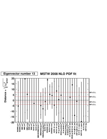
This suggests that likelihood contours (for example one-) for the global fit can only be determined while simultaneously testing for the degree of agreement of individual experiments with it. The way this is done is by introducing the concept of “tolerance”, defined as follows [76]. First, the Hessian matrix is diagonalized. Next, one moves the value of each eigenvector away from the minimum of the global fit in either direction, and one computes the of each experiment. Then, for each experiment one determines both the position of the minimum of the and the one- interval about it (corresponding to the variation about the minimum), or equivalently the 90% confidence level (obtained by rescaling the former interval by the factor [34]). Finally, one takes the envelope of the error bands for individual experiments at the desired confidence level (c.l., henceforth). For example, at the 90% c.l. one determines the range of variation in parameter space along this eigenvector about the minimum such that the 90% c.l. interval of each experiment overlaps with this range. This gives a tolerance interval for the given eigenvector. The width of this interval can be measured in units of the variation of the of the global fit. This defines a tolerance: is the width of the envelope (see Fig. 18).
The 90% c.l. is finally taken to be instead of (equivalently, the one contour is ). The logic behind this is that PDFs should allow one to obtain predictions for new processes at the desired confidence level: for instance, the actual result for a new measurement should have a 68% chance of actually falling into the predicted one- band. If new experiments behave as the experiments which are already included in the fit do on average, then this will happen for the one- band defined in this way, while if the one- band were defined on the basis of standard statistics the chances of the measurements falling outside the band would be much higher. It should be stressed that therefore a tolerance analysis is required in order for a fit based on this methodology to be reliable (unless the dataset adopted is very small and/or consistent).
In Ref. [76] it was found that in practice worked for all eigenvalues and experiments at 90% c.l. for the dataset and fit considered there, corresponding to at one sigma. A similar analysis in Ref. [77] found instead . Taken at face value, this would imply that all experimental uncertainties have been underestimated by a factor of about (for ) or (for ) . While some uncertainty underestimation is possible, such a large factor is at best puzzling, and thus its origin deserves further investigation.
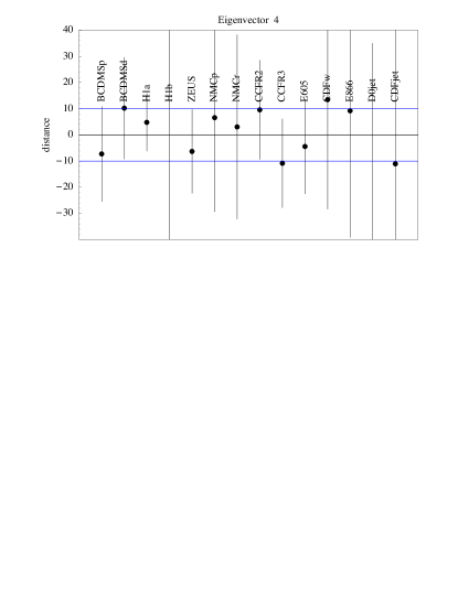
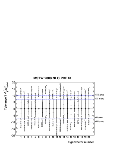
The concept of tolerance was subsequently refined, by suggesting that instead of a global tolerance value for all eigenvalues, a different tolerance value, determined as above, be adopted along each eigenvector direction. This is called “dynamical” tolerance [30]. Proceeding in this way, one finds a tolerance , with most values being in the range , so the large tolerance problem is somewhat mitigated. Also, in this approach it is possible to trace which individual experiment is controlling the tolerance range for each eigenvalue. This, together with the expression of the eigenvector in terms of the original parameters, provides insight on the relation between data and PDF parameters and their mutual consistency. Such an analysis is displayed in Fig. 19, where both the tolerance analysis for one specific eigenvector, and then the experiments and corresponding band which control the tolerance interval for each eigenvector. A related but different refinement was suggested in Ref. [28], based on the idea of determining the band such that each experiment agrees with the global fit to say 90% c.l. by means of a sharply rising penalty term in the global based on the of each experiment.
It is interesting to contrast this treatment of uncertainties in the Hessian approach with “standard” parametrization with the Monte Carlo approach together with neural network parametrization discussed in Sect. 3.2.2. In that approach, uncertainty bands corresponding to any given confidence level can be computed directly from the Monte Carlo sample: the one- interval is just the standard deviation of the sample, and one may even check whether it indeed corresponds to the central 68% of the distributions of PDF replicas. This is shown in Fig. 20 for the gluon distribution (from Ref. [38]): in this case (and in fact [41] in most cases) the one- and 68% c.l. intervals coincide. In a Monte Carlo approach, whether or not the fits behave consistently when comparing fit results to new data, and then including these new data into the fit, can be verified a posteriori by performing statistical tests on the fit results. These tests were performed successfully for the fits of Refs. [38, 53, 41].
The question of the appropriate range in global which corresponds to one sigma is thus side-stepped. In principle, it can be answered a posteriori: in a Monte Carlo approach, the of the mean is a property of the Monte Carlo sample, so one could compute the one- interval from the sample itself. In practice, it is nontrivial to do this accurately because, as explained in Sect. 31, the has fluctuations of order , and in a Monte Carlo approach these fluctuations take place replica by replica, so one needs a very large sample to determine the accurately.
However, the issues which may be responsible for the large tolerances can be addressed both in a Hessian and in a Monte Carlo approach as we will now discuss.
5.2 Parametrization bias and data incompatibility
The large tolerance values discussed in Sect. 5.1 are, by definition, a manifestation of the poor mutual compatibility of the experiments that go into the global fit. One possible explanation for this is that experiments are genuinely incompatible with each other within their stated uncertainties, i.e. that their published uncertainties are underestimated. We will refer to this possible explanation as “data incompatibility”.
Another possible explanation is that the way uncertainties are propagated from experiments onto PDFs leads to underestimating the uncertainty in the latter. For example, assume that experiment does not depend on some PDF parameter, and that one determines PDFs from this experiment, but instead of leaving the undetermined parameter free, one fixes it in some arbitrary way. If the ensuing PDF is then used to predict another experiment B which happens to depend on the undetermined parameter the likelihood of results being in agreement with the prediction will not depend on statistics, but rather in the arbitrary way the parameter has been fixed. We will refer to this as “parametrization bias”.
Of course other options are possible: for example, that the theory which is being used is not adequate. In the latter case, however, one would have to find a convincing argument why this theoretical inadequacy has not been seen elsewhere.
Data incompatibility in the Hessian approach was recently studied in a quantitative way in Ref. [79], exploiting the observation [80] that once the has been written in the form of Eq. (32) one can perform a further linear transformation of the parameters which preserves this form, while also diagonalizing the contribution to the from some specific subset of data. After this simultaneous diagonalization, the is written as the sum of a contribution from the data in the given subset and the rest: the distance of the minima of these two contributions to the in units of the corresponding standard deviation measures the compatibility of the given subset of data with the rest of the global dataset. The idea is then to study the distribution of such distances, in all cases in which the experiment does contribute significantly to the global minimum. If experimental uncertainties are correctly estimated, they should be gaussianly distributed. The results of this analysis, shown in Fig. 21, suggest that the distribution of discrepancies deviates significantly from a gaussian distribution, and that if it is fitted to a gaussian its uncertainty should be rescaled by about a factor 2. This suggests uncertainty underestimation by a similar factor, which corresponds to a value of the tolerance for 90% c.l. of order of .

This suggest that data incompatibility can explain only in part the need for large tolerance. Further evidence that data incompatibility is at most moderate can be obtained in a Monte Carlo approach, by comparing the effect of the subsequent inclusion of different datasets into a fit. Indeed, if some datasets were incompatible with others, then the effect of their inclusion in the global fit would change according to whether the global fit already includes the data with which they are incompatible or not. Assume for example that the gluon determined from jets is compatible with that found exploiting scaling violations in DIS data, but less compatible with that found from scaling violations in Drell-Yan: then, inclusion of jet data in a pure DIS fit would have a different effect than their inclusion in a fit which contains both DIS and Drell-Yan. When such tests are performed [41] no evidence for data incompatibility is found, as demonstrated in Fig. 22).
Let us now turn to the possibility that parameterization bias may be responsible for the effect. The way this could happen in a Hessian approach was recently exemplified in Ref. [81]. Assume a relevant parameter on which PDFs depend is not fitted, but rather fixed by assumption at a value which is away from its best-fit. Then, clearly (see Fig. 23) the one- range for the other parameters when this parameter is kept fixed corresponds to a variation of which is greater than the standard found when moving away from the minimum. A first estimate of the possible size of this effect was also provided in Ref. [81] by simply repeating the PDF fit of Ref. [27], but with a much more general parametrization, based on expanding the gluon on a basis of orthogonal polynomial, analogous to that of Ref. [24] shown in Fig. 9. With this more general parametrization, fits whose is similar to or better than the best-fit of the more restrictive parametrization are found to span a band which corresponds roughly to the range for the restrictive parametrization. So this suggests a tolerance of at least just to account for the bias on the gluon shape imposed by the parametrization of Ref. [27]
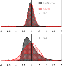
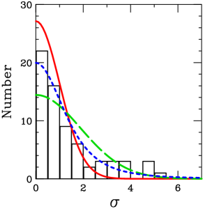
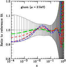
The issue of parton parametrization and bias thus deserves further investigation. First, one may ask whether the gaussian assumption is by itself a source of bias. This has been investigated in Ref. [23], using a Monte Carlo approach together with a standard parton parametrization. Data replicas based on the HERA DIS data ( of Fig. 7) have been generated either using a gaussian or a lognormal distribution (see Fig. 24), and used for a PDF fit based on the “standard” functional form Eq. (26). In each case, both the Monte Carlo and Hessian uncertainty are computed. Results are shown in Fig. 24: the lognormal and gaussian results are essentially indistinguishable, and so are the Hessian and Monte Carlo uncertainties. The choice of the probability distribution of the data does not seem to play any major role, as one might have expected from the central limit theorem: with so many data, everything looks gaussian. This also provide a nice visual demonstration of the equivalence of Hessian and Monte Carlo uncertainty computation in the Gaussian case.
On the other hand, in the same figure we also show the gluon obtained in a fit to exactly the same data, but using the neural network functional form and associate cross-validation methodology of Ref. [53]. It is clear that the uncertainty is now much wider. This suggests that it is the form of parametrization which plays a dominant role, rather than the form of the probability distribution.
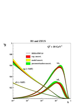
The issue has been investigated further in the HERAPDF [29] PDF fits, where the standard PDF uncertainty based on a “standard” functional form Eq. (26) has been supplemented by a further parametrization uncertainty, obtained by varying the assumed functional form (in particular, the large behaviour, the number of terms in the polynomial Eq. (27), and the assumptions on strangeness which is not fitted). It is clear from Fig. 25 that this leads to a sizable enlargement of the PDF uncertainty band.
The Monte Carlo approach together with neural network offers an interesting way of searching for the origin of uncertainties, in that different sources of uncertainty can be switched on and off one at a time. In particular, one may perform the following exercise. First, one freezes the generation of data replicas, and one takes each replica dataset equal to the central values of the data. Recall from Sect. 3.2.2 that each replica is fitted to a different, randomly chosen subset of the data. Hence, all datasets of Fig. 7 are now the same, and only the way they are partitioned in validation and training sets changes between replicas. Each PDF replica is thus obtained as the fit to a different partition of the central experimental data. The (square) fluctuation of the data are reduced by a factor two: instead of having replicas which fluctuate about experimental data which in turn fluctuate about their “true” values, one only has different subsets of central data fluctuating about their true values.
| replicas | central value | fixed partition | |
| 1.32 | 1.32 | 1.3 | |
| 0.039 | 0.035 | 0.03 |
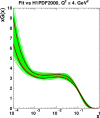
In Tab. 2 we compare some indicators of fit quality and results for a fit obtained in this way to those of the corresponding standard fit (using the fit of Ref. [38], based on DIS data). In particular, we compare the of the best fit in either case: this is unchanged. However, the average of each replica fit is smaller by a factor two. This is as it should be: in both cases the best-fit is reproducing the same central best-fit value, but the fluctuation of replicas about it are now suppressed by a factor two, and thus the average per replica is reduced by approximately the same factor. The surprising result however is found when one computes the average percentage uncertainty in the prediction obtained in either case. This is determined as the percentage uncertainty of the prediction obtained from the final replica PDF set, for all datapoints included in the fit, averaged over datapoints. One might expect that having halved the fluctuations, the average uncertainty should be reduced by a factor ; in actual fact, it is reduced by a much smaller amount.
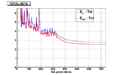
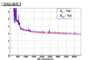
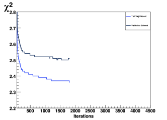
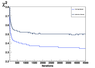
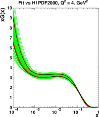
The origin of this state of affairs can be understood by performing an even more extreme text: one simply produces 100 replicas fitted to exactly the same partition of the central data. In this case, all contain the same data, partitioned in the same way into training and validation sets. Naively one may think that this may lead to simply repeating 100 times the same fit. This is not necessarily the case because each replica is determined by initializing the neural networks at random, and then minimizing by means of an (equally random) genetic algorithm. Hence one starts each time from a different point in the very wide parameter space, and then the minimum is approached along a different path. Indeed, in Fig 26 we show the profiles along the minimization, as a function of the number of iterations of the minimization algorithm, for two individual replicas: it is clear that even though the final values are quite similar, the number of iterations and profiles that take there are quite different, thereby showing that the minimum is approached along different paths.
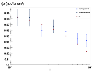
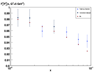
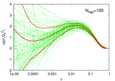
In this case, in order to make sure that results do not depend on the particular partition that has been picked in the first place, the whole procedure is repeated five times with five different choice of starting partition and results are then averaged. Results are shown in Tab. 2 (they should be taken as indicative, because one should use rather more than five fixed partitions for accurate results). These results are quite surprizing. The of the best fit and the average over replicas are unchanged, and this is to be expected: it shows that indeed the five replicas chosen are not special. However, very surprizingly, the average uncertainty, which one might expect to be tiny, is more than 50% of that of the original fit. This is also seen by comparing results for PDFs (see Fig. 27: the uncertainty band is smaller, but of the same order of magnitude as that of the full fit. The inevitable conclusion is that a large fraction of the uncertainty band, probably more than half, does not depend on the fluctuations in the data. Rather, it is a consequence of the fact that there is an infinity of functions that provide fits of comparable quantity to the data. Different minimization profiles such as those shown in Fig. 26 land on somewhat different minima; the uncertainty of this fit is then a measure of the spread of this space of minima. Once understood that a sizable fraction is simply due to this “functional” uncertainty, it is clear why it is more difficult to capture with a fixed parametrization, which then requires a suitable tolerance in order to mimic it.
6 Recent developments
The state of the art in PDF determination is moving very fast and thus any attempt to review it would necessarily become obsolete quite rapidly: a recent review of the status of the field as of November 2010 is in Ref. [83]. Here, in an attempt to discuss issues of somewhat less fleeting value, we will first briefly review theoretical uncertainties, which are the current frontier of PDF determination, then summarize what progress has been made and what remains to be done in the determination of PDFs for the LHC in the years to come.
6.1 Theoretical uncertainties
As already mentioned, the PDF uncertainties discussed in Sect. 5 are the result of propagating into the space of PDFs the uncertainty on the data on which the PDF determination is based. Most of the effort has gone so far in their determination and understanding because they are likely to be at present the dominant uncertainty. However, it has been recently realized that in many cases uncertainties related to the theory used to extract PDFs from the data may be larger than one may think. These, as already mentioned, include both uncertainties in the theory itself (such as higher order corrections) but also uncertainties in the knowledge of the free parameters on the theory.
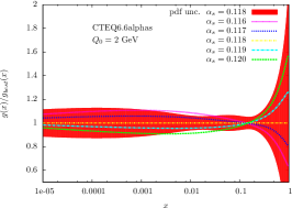
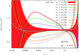
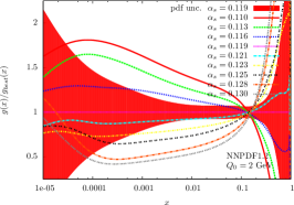
The most obvious source of theoretical uncertainty is the value of the strong coupling . The PDF which depends most strongly on it is the gluon distribution, which, as discussed in Sect. 4.4 is largely determined by scaling violations: the rather strong dependence of the gluon on the value of is shown in Fig. 28 for various PDF sets. Note that even though, as discussed in Sect. 3.1 the total PDF+ uncertainty can be obtained by determining these two uncertainties separately and adding results in quadrature [35], when determining the uncertainty, the value of in the factorization formula Eq. (2.1) must be varied both in the PDFs and in the partonic cross section . This is especially important when dealing with processes, such as Higgs production in gluon-gluon fusion [85, 83] (or also top production) which depend on the gluon PDF and start at a high order in . For this purpose, PDF sets corresponding to different values of are necessary and have thus been produced by several group (using sets with PDFs given as a continuous function of is in principle also possible, but practically more cumbersome and less accurate).
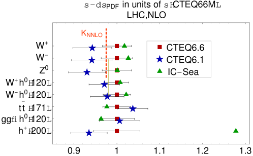
The only other free parameters in the QCD Lagrangian are the quark masses, i.e., in the perturbative regime, the heavy quark masses. Dependence of PDFs on them are larger than one might naively expect, and has two different origins which we will now discuss in turn. The first, is simply the fact that even though all perturbative computation are done up to power-suppressed terms in , terms of order and may have a non-negligible impact on PDF fits. This was brought to general attention by the comparison [27] of two calculations of the and production cross-sections based on PDF sets which differ mostly because one does include corrections (CTEQ6.1 [86]) while the other (CTEQ6.6 [27]) does not. It turns out (see Fig. 29) that these corrections change the result by an amount which is almost twice the (statistical) PDF uncertainty (as defined in Sect. 5): note that all the bands in Fig. (29) are at 90%c.l., and the one- intervals would be accordingly smaller.
In order to understand what is going on here, one must recall the way heavy quark PDFs are defined, and heavy quarks are treated in perturbative QCD computations. Usually, perturbative QCD computations are performed in a decoupling renormalization scheme [87], in which heavy quarks decouple from perturbative Feynman diagrams for scales much lower than the quark mass. In such a scheme, below threshold the number of flavours in the evolution equation for the strong coupling and for parton distributions Eq. (22) is equal to the number of light flavours. So in particular whereas there may still exist a non-perturbative nonvanishing “intrinsic” heavy quark PDF below threshold [19], it will only start evolving and coupling to other PDFs through evolution equations above threshold: for all practical purposes, below charm threshold . However, for scales which are much larger that the heavy quark mass, there is no reason to treat the heavy quark on a different footing from any other light quark: for scales much larger than the charm mass, all terms of order can be neglected, and there are massless flavours. The problem arises for scales which are higher but not much higher than the heavy quark mass: then, the heavy quark can be produced and it does not decouple, yet it is not necessarily a good approximation to treat it as massless, i.e. to neglect corrections.
This situation is illustrated in Fig. 30, where we show the neutral-current photon-induced DIS structure function (i.e. the contribution to in which the virtual photon couples to a charm quark) computed in various approximations. The two curves labelled ZM-VFN (purple, highest curves) are curves in which charm is simply treated as another massless flavour. The charm PDF is assumed to vanish below threshold, and above threshold a (massless) charm component is generated by perturbative evolution — note that even if an intrinsic component did exist, it should be small, and only non-negligible for very large [19]. The two NLO and NNLO ZM-VFN (zero mass-variable flavour number) curves correspond to the case in which anomalous dimensions are computed up to and respectively: the solution to evolution equations then includes all contributions of order to all orders in , with at NLO and with at NNLO. They are called “variable flavour number” curves because the number of active flavours is increased by one unit when each heavy quark threshold is crossed. For light quarks, — the starting scale of perturbative evolution — and for the charm contribution . Given that , at high scale there is no reason not to include the charm contribution in evolution equations along with the light contributions.
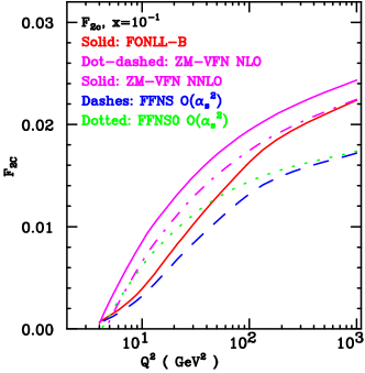
However, the evolution equations neglect all quark mass effects. Indeed, the curve labelled FFN (fixed flavour number) shows the result of the computation fixed order in , but now with the dependence on fully included. This is a fixed-flavour number result because charm is included as a massive quark in partonic cross sections, but only the lighter flavours contribute to evolution equations and the running of . Its limit for , which coincides with the contributions to the VF-ZFN NNLO, but up to only, is labelled as FFN. The FFN and FFN results are different, and their difference, which is sizable for GeV2 is a measure of the size of mass suppressed contributions (note however that all curves come together at threshold, where vanishes). In this region, is not large and indeed the ZM-VFN NNLO curve and the FFN are quite close: the inclusion of higher order powers of in the ZM-VFN NNLO has little effect. On the other hand, for GeV2 the FFN and FFN curve become quite close — their difference are mass-suppressed contributions which here have little effect — but the ZM-VFN curve is much higher: here is large and its all-order inclusion in the ZM-VFN result is important. In fact, the difference between the FFN curve and the ZM-VFN curve is much larger than the difference between the NLO and NNLO ZM-VFN curves: it is important to resum to all orders, but whether this resummation is done to NLO or NNLO has a much smaller impact.
So summarizing: for lower GeV2 it is important to include mass corrections and not important to resum to all orders, so the most accurate result is the FFN one. For GeV2 the converse is true and the most accurate result is the ZM-VFN one. The question is whether the two can be combined. That this is possible in principle to any perturbative order is a consequence of a factorization theorem for massive quarks proven to all orders in Ref. [88]. A practical implementation was suggested and worked out up to NLO in Ref. [89] - the so-called ACOT method, which was used to produce the massive CTEQ6.6 result of Fig. 29. Other implementations were suggested in Refs. [90, 91] (TR method) for deep-inelastic scattering, and in Ref. [92] for hadroproduction (FONLL method, recently generalized to DIS and worked out up to NNLO in Ref. [93]). These various methods, which thus combine both a massive fixed-order FFN computation and a massless all-order ZM-VFN resummation, are often referred to as “GM-VFN” (general mass, variable flavour number) methods.
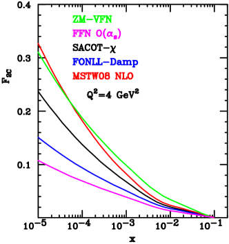
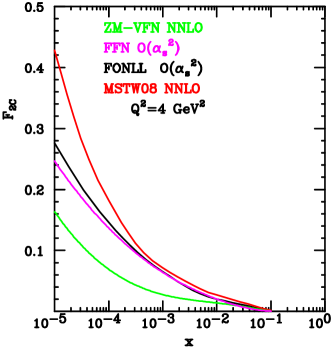
The FONLL curve is also shown in Fig. 30, in a version (called FONLL-B) which includes all terms which are contained in the ZM-VFN NLO and FFN calculations. It is clear that the FONLL-B curve nicely interpolates between the FFN curve, more accurate at low scale, and the ZM-VFN one, more accurate at high scale. Without entering a discussion of these various prescriptions, which would be quite technical, it is important to understand that (unless an error is made) all GM-VFN prescriptions include all the terms included in the ZM-VFN and FFN calculations: they may differ first, in the orders at which either of the ZM-VFN and FFN terms are included, and furthermore, because even with the same terms included, subleading terms are generally different, and may in practice have a non-negligible impact. The impact of these subleading terms can only be reduced by pushing to higher orders both the ZM-VFN and FFN contributions which are included in the GM result. This is illustrated in Fig. 31, where the FFN, ZM-VFN and GM-VFN results are compared. The GM-VFN are shown in the version adopted by CTEQ6.6 Ref. [27] of the ACOT method of Ref. [89] (only available at NLO), in the version adopted by MSTW08 [30] of the TR method of Refs. [90, 91], and with the FONLL method of Ref. [93]. It is clear that the differences between the various GM schemes are sizable, and only start decreasing at NNLO-.
Considerable progress has been made recently in the benchmarking of all these GM schemes (see Ref. [94]), and the use of a GM-VFN scheme, which is highly desirable, has become more widespread. However, a systematic estimate of the uncertainties related to the choice of specific heavy quark scheme is not available in existing PDF sets.
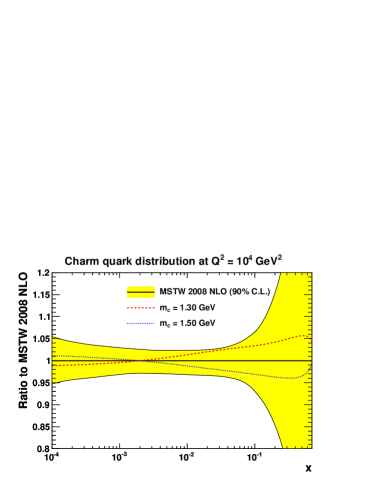
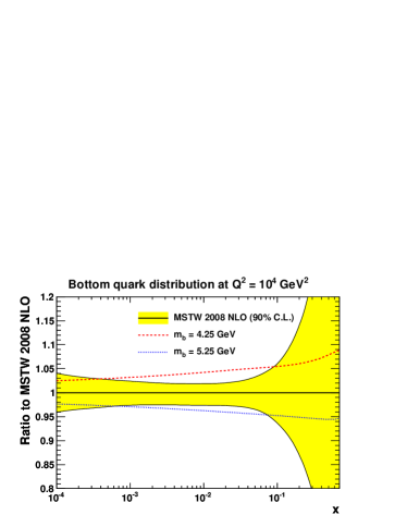
So far we have only discussed one of the two ambiguities related to the treatment of heavy quarks. The other one has simply to do with the value of the heavy quark mass. This has a considerable impact because, as we have seen, apart from possible intrinsic contributions, heavy quark PDFs are obtained by assuming them to vanish at threshold, and then to be generated by perturbative evolution. But changing the mass changes the position of the threshold, and thus the amount of evolution. This has been very recently argued to have a potentially non-negligible impact on phenomenology [96]. First PDF sets with variable values of the heavy quark masses have been presented in Ref. [95]. Some representative results are shown in Fig 32: when the heavy quark masses are varied in a range which is representative of their uncertainty, the heavy PDFs vary by an amount (more than 5%) which is of the same order or larger than the PDF uncertainty. This variation then propagates onto all other PDFs and especially the gluon, both due to mixing upon perturbative evolution, and to sum rules.
It seems clear that for accurate phenomenology the values of the heavy quark masses will have to be treated analogously to what is now being done for the strong coupling: PDF sets with varying heavy quark masses will have to be provided, and the value of the masses will have to be varied simultaneously in the partonic cross section and in the PDF sets.
Finally, it should be recalled that there is at present no reliable estimate of the effect on PDFs of the uncertainty due to the truncation of the perturbative expansion. This is possibly a relatively smaller effect in comparison to those we discussed so far, but this too will have to be included in PDF sets, for example by providing sets which correspond to different values of the renormalization and factorization scales, whose variation is a way of estimating unknown higher order corrections. All in all, a proper treatment of theoretical uncertainty is the current frontier in PDF uncertainties.
6.2 PDFs for the LHC
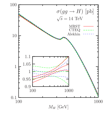
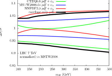
An ideal PDF determination should include all of the following features:
-
•
It should be based on a dataset which is as wide as possible in order to ensure that all relevant experimental information is retained; in particular, all processes discussed in Sect. 4 should be used.
-
•
It should be based on a sufficiently general and unbiased parton parametrization and/or it should include a careful estimate of the effect of varying the parton parametrization.
-
•
It should provide PDF uncertainty bands which have been either a priori (tolerance) or a posterior (Monte Carlo) checked to provide consistently-sized confidence levels for individual experiments.
-
•
It should include heavy quark mass effects through a GM-VFN scheme, and provide an estimate of the uncertainties due to subleading terms not included in the scheme which has been adopted.
-
•
It should be based on computations performed at the highest available perturbative order, namely NNLO for evolution equations and for most or all of the processes used for PDF determination.
-
•
It should provide PDFs for a variety of values of , reasonably thinly spaced and in a range which is representative of the uncertainty on this parameter.
-
•
Ditto for the values of heavy quark masses.
-
•
It should include an estimate of uncertainties related to the truncation of the perturbative expansion.
At present, there exists no PDF determination which has all these features simultaneously. Which of these features is most important for accurate results it will be possible to say with certainty only after such a PDF determination is constructed. However, the various features have been listed in the approximate (decreasing) likely order of importance, at least in the opinion of this author, based on the arguments presented so far.
Therefore, existing sets satisfy only some of these requirements. Current PDF sets are provides through a standard interface, LHAPDF [98], which is regularly updated for the inclusion of new sets and updates. Current PDF sets and their salient features include the following (listed in order of decreasing number of datasets included)
-
•
MSTW08 [30, 84, 95] Latest in the MRS-MRST-MSTW series of fits (Ref. [99] and subsequent papers). All data of Sect. 4, plus HERA DIS jets. Hessian approach with parametrization Eq. (26) for seven independent PDFs (three lightest flavour and antiflavours and the gluon); 28 free parameters, 8 of which are held fixed in the determination of uncertainties; dynamical tolerance uncertainties. GM-VFN scheme. Results available for various values of , and . NNLO perturbative order (whenever available).
-
•
CT10 [28] Latest in the CTEQ series of fits (Ref. [100] and subsequent papers, see also [101]). All data of Sect. 4. Hessian approach with parametrization Eq. (26) for six independent PDFs (two lightest flavour and antiflavours, total strangeness and the gluon); 26 free parameters; dynamical tolerance uncertainties. GM-VFN scheme. Results available for various values of . NLO perturbative order.
-
•
NNPDF2.0 [41] Latest in the NNPDF series of fits (Ref. [45] and subsequent papers). All data of Sect. 4. Monte Carlo approach with neural network parametrization for seven independent PDFs (the three lightest flavours and antiflavours, total strangeness and the gluon); 259 () free parameters; cross-validation uncertainties. ZM-VFN scheme. Results available for various values of . NLO perturbative order.
-
•
JR [102] Latest in the GR-GRV-GJR series of fits (Ref. [103] and subsequent papers). All data of Sect. 4 except and production. Hessian approach with parametrization Eq. (26) for five independent PDFs (two lightest flavour and antiflavours and the gluon); 20 free parameters; fixed tolerance uncertainties. Results available for single value of , but Hessian includes . FFN scheme. NNLO perturbative order.
-
•
ABKM [104] Latest in the Alekhin series of fits (Ref. [73] and subsequent papers). All DIS data of Sect. 4 and fixed-target virtual photon Drell-Yan production. Hessian approach with parametrization Eq. (26) for six independent PDFs (two lightest flavour and antiflavours, total strangeness and the gluon); 21 free parameters; no tolerance (). Results available for single value of , but Hessian includes , and also heavy quark masses. FFN scheme. NNLO perturbative order.
-
•
HERAPDF1.0 [29] HERA only DIS data Hessian approach with parametrization Eq. (26) for five independent PDFs (two lightest flavour and antiflavours, and the gluon); 10 free parameters; no tolerance() but inclusion of parametrization uncertainties. GM-VFN scheme. Results available for various values of . NNLO perturbative order.
Detailed comparisons of these PDF sets is the subject of ongoing benchmarking exercises, with the aim of arriving at the most accurate common determination of PDFs. The successfulness of the enterprise can be gauged by putting side by side (see Fig. 33) predictions for Higgs production via gluon-gluon fusion at the LHC with different PDF sets obtained as the first PDF with uncertainties were published [78], with those obtained more recently as first collisions were taking place at the LHC [85] (see Fig. 33). The improvement is quite clear, and convergence between PDF sets has further improved since.
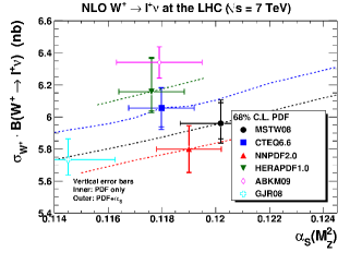
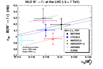
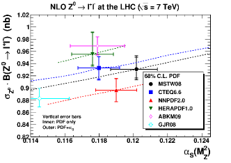
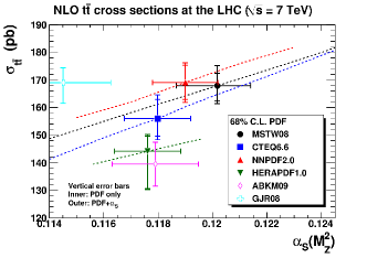
The status of the computation of the simplest LHC processes (which have been suggested as “standard candles”, e.g. as a means to measure the machine luminosity [106]) is summarized in the plots of Fig. 34, where predictions for , and top total cross sections obtained at NLO using the ABKM09 [104], CTEQ6.6 [27], HERAPDF1.0 [29], GJR08 [107], MSTW08 [30] and NNPDF2.0 [41] sets are plotted as a function of . The dotted lines show how each prediction can be extrapolated to different values of (the extrapolation is not available for the ABKM and GJR sets since these are only published for a single value of , though in principle the information on the dependence is contained in their covariance matrix). It is clear that first, once brought to a common value of the various sets are in fair agreement, and second, the agreement further improves when restricted to PDF sets that are based on more similar assumptions (such as common dataset, number of independent PDFs etc.).
An interesting question that remains is how one can proceed when some disagreement remains, and there is no clear reason to favor one set over the other. In this case, Bayesian statistics provides an answer [108]: in Bayesian terms, the probability distribution for PDFs is a distribution of true values, i.e. expresses the degree of belief that the true value is indeed . Then, given two different, but a priori equally reliable determinations and of the probability distribution, the combined probability is just , with obvious generalizations if the determinations of the probability distribution are more than two or not all equally likely. In a Monte Carlo approach this is especially easy to implement: the combined probability distribution is obtained by simply taking a Monte Carlo sample in which half of the replicas come from either distribution. A 68%c.l. of the combined probability is then simply the region which contains the central 68% of all the given distributions, i.e. 68% of the combined replica set.
In practice, a reasonable approximation to the Bayesian estimate may well consist of simply taking the envelope (i.e. the union) of the 68% intervals of the probability distributions which are being combined: this typically leads to a slight overestimate of the error band, because some of the replicas in the outer 32% of one of the distribution may fall within the central 68% of another distribution, but this in practice is often a small correction, hence the envelope prescription can be a simple and effective way of combining probability distributions.
7 Conclusion
The physics of parton distributions is now close to a beginning, rather than a conclusion: LHC data for many of the processes discussed in Sect. 4 are being collected and will soon be published. The availability of LHC data is likely to change significantly our perspective on the subject. The kinematic range of “old” processes such as Drell-Yan will be extended and their accuracy will improve. Processes which are at present not competitive will become important (such as perhaps prompt photon production). Entirely new processes will play a role, such as Higgs production. Hopefully, classes of new physical processes will be discovered: whatever their nature, they will be observed in proton collisions, and thus pose new challenges to our understanding of the nucleon. It may turn out that an interplay with new machines, such as an electron-proton LHeC collider [109], or perhaps even a neutrino factory [42] may be necessary in order to exploit fully the LHC potential. A review of this subject written ten years from now is likely to be quite different from the present one, and possibly much more interesting.
Acknowledgements: I am grateful to the organizers of the Zakopane school and especially Michał Praszałowicz for giving me the privilege to present these lectures, and I thank all participants and lecturers, in particular Paul Hoyer, for their interest and critical input. My understanding of this subject was shaped by many discussions, especially within the PDF4LHC workshop [17]: I would like to thank in particular A. de Roeck, A. Glazov, J. Huston, P. Nadolsky, J. Pumplin, R. Thorne. I also thank all the members of the NNPDF collaboration and especially J. Rojo for innumerable discussions on the subject of these lectures. This work was partly supported by the European network HEPTOOLS under contract MRTN-CT-2006-035505.
References
- [1] G. Altarelli, “QCD: The theory of strong interactions,” In *Landolt-Boernstein I 21A: Elementary particles* 4
- [2] M. Klein and R. Yoshida, “Collider physics at HERA,” Prog. Part. Nucl. Phys. 61 (2008) 343 [arXiv:0805.3334 [hep-ex]].
- [3] M. L. Mangano, “Understanding the standard Model, as a bridge to the discovery of new Int. J. Mod. Phys. A 23 (2008) 3833 [arXiv:0802.0026 [hep-ph]].
-
[4]
G. Arnison et al. [UA1 Collaboration],
“Experimental observation of isolated large transverse energy electrons
with associated missing energy at s**(1/2) = 540-GeV,”
Phys. Lett. B 122 (1983) 103;
G. Arnison et al. [UA1 Collaboration], “Experimental observation of lepton pairs of invariant mass around 95-GeV/at the CERN SPS collider,” Phys. Lett. B 126 (1983) 398;
M. Banner et al. [UA2 Collaboration], “Observation of single isolated electrons of high transverse momentum in events with missing transverse energy at the CERN anti-p p collider,” Phys. Lett. B 122 (1983) 476;
P. Bagnaia et al. [UA2 Collaboration], “Evidence for Z0 e+ e- at the CERN anti-p p collider,” Phys. Lett. B 129 (1983) 130. - [5] G. Arnison et al. [UA1 Collaboration], “W production properties at the CERN SPS Collider,” Lett. Nuovo Cim. 44 (1985) 1.
-
[6]
G. Altarelli, R. K. Ellis, M. Greco and G. Martinelli,
“Vector boson production at colliders: a theoretical reappraisal,”
Nucl. Phys. B 246 (1984) 12;
G. Altarelli, R. K. Ellis and G. Martinelli, “Vector boson production at present and future colliders,” Z. Phys. C 27 (1985) 617. - [7] M. Gluck, E. Hoffmann and E. Reya, “Scaling violations and the gluon distribution of the nucleon,” Z. Phys. C 13 (1982) 119.
- [8] D. W. Duke and J. F. Owens, “ dependent parametrizations of parton distribution functions,” Phys. Rev. D 30 (1984) 49.
- [9] E. Eichten, I. Hinchliffe, K. D. Lane and C. Quigg, “Super collider physics,” Rev. Mod. Phys. 56 (1984) 579 [Addendum-ibid. 58 (1986) 1065].
- [10] W. K. Tung, “Status of global QCD analysis and the parton structure of the nucleon,” arXiv:hep-ph/0409145.
- [11] C. F. Berger and D. Forde, “Multi-parton scattering amplitudes via on-shell methods,” arXiv:0912.3534 [hep-ph].
- [12] S. Weinzierl, “Introduction to feynman integrals,” arXiv:1005.1855 [hep-ph].
- [13] G. P. Salam, “Towards jetography,” Eur. Phys. J. C 67 (2010) 637 [arXiv:0906.1833 [hep-ph]].
- [14] P. Nason, “Recent developments in POWHEG,” PoS RADCOR2009 (2010) 018 [arXiv:1001.2747 [hep-ph]].
- [15] S. Alekhin et al., “HERA and the LHC - A workshop on the implications of HERA for LHC physics: Proceedings Part A,” arXiv:hep-ph/0601012; “Part B,” arXiv:hep-ph/0601013.
- [16] Z. J. Ajaltouni et al., “Proceedings of the workshop: HERA and the LHC workshop series on the implications of HERA for LHC physics,” arXiv:0903.3861 [hep-ph].
-
[17]
A. de Roeck, “The PDF4LHC initiative”, Sect. 6 in
Ref. [82];
http://www.hep.ucl.ac.uk/pdf4lhc - [18] R. K. Ellis, W. J. Stirling and B. R. Webber, “QCD and collider physics,” Camb. Monogr. Part. Phys. Nucl. Phys. Cosmol. 8 (1996) 1.
- [19] S. J. Brodsky, P. Hoyer, C. Peterson and N. Sakai, “The intrinsic charm of the proton,” Phys. Lett. B 93 (1980) 451.
- [20] M. Gluck and E. Reya, “Operator mixing and scaling deviations in asymptotically free field theories,” Phys. Rev. D 14 (1976) 3034.
- [21] P. W. Johnson and W. k. Tung, “Comparison of asymptotically free theories with high-energy deep inelastic scattering data,” Nucl. Phys. B 121 (1977) 270.
- [22] S. Forte, L. Garrido, J. I. Latorre and A. Piccione, “Neural network parametrization of deep-inelastic structure functions,” JHEP 0205 (2002) 062 [arXiv:hep-ph/0204232].
- [23] J. Feltesse, A. Glazov and V. Radescu, “Experimental error propagation”, Sect 3.2 in Ref. [82]
-
[24]
V. Radescu, talk at “PDF4LHC”, DESY, November 2009;
A. Glazov, S. Moch and V. Radescu, “Parton distribution uncertainties using smoothness prior,” arXiv:1009.6170 [hep-ph]. - [25] S. J. Brodsky and G. R. Farrar, “Scaling laws at large transverse momentum,” Phys. Rev. Lett. 31 (1973) 1153.
- [26] H. D. I. Abarbanel, M. L. Goldberger and S. B. Treiman, “Asymptotic properties of electroproduction structure functions,” Phys. Rev. Lett. 22 (1969) 500.
- [27] P. M. Nadolsky et al., “Implications of CTEQ global analysis for collider observables,” Phys. Rev. D 78 (2008) 013004 [arXiv:0802.0007 [hep-ph]].
- [28] H. L. Lai, M. Guzzi, J. Huston, Z. Li, P. M. Nadolsky, J. Pumplin and C. P. Yuan, “New parton distributions for collider physics,” Phys. Rev. D 82 (2010) 074024 [arXiv:1007.2241 [hep-ph]].
- [29] F. D. Aaron et al. [H1 and ZEUS Collaboration], “Combined measurement and QCD analysis of the inclusive ep scattering cross sections at HERA,” JHEP 1001 (2010) 109 [arXiv:0911.0884 [hep-ex]].
- [30] A. D. Martin, W. J. Stirling, R. S. Thorne and G. Watt, “Parton distributions for the LHC,” Eur. Phys. J. C 63 (2009) 189 [arXiv:0901.0002 [hep-ph]].
- [31] G. D’Agostini, “On the use of the covariance matrix to fit correlated data,” Nucl. Instrum. Meth. A 346 (1994) 306.
- [32] R. D. Ball, L. Del Debbio, S. Forte, A. Guffanti, J. I. Latorre, J. Rojo and M. Ubiali [NNPDF Collaboration], “Fitting parton distribution data with multiplicative normalization uncertainties,” JHEP 1005 (2010) 075 [arXiv:0912.2276 [hep-ph]].
- [33] G. Cowan, “Statistical data analysis,” Oxford, UK: Clarendon (1998)
- [34] Sect. 33 in: K. Nakamura [Particle Data Group], “Review of particle physics,” J. Phys. G 37, 075021 (2010).
- [35] H. L. Lai, J. Huston, Z. Li, P. Nadolsky, J. Pumplin, D. Stump and C. P. Yuan, “Uncertainty induced by QCD coupling in the CTEQ global analysis of parton distributions,” Phys. Rev. D 82 (2010) 054021 [arXiv:1004.4624 [hep-ph]].
- [36] M. Hirai et al. [Asymmetry Analysis Collaboration], “Uncertainty of polarized parton distributions,” Int. J. Mod. Phys. A 18 (2003) 1203.
- [37] J. C. Collins and J. Pumplin, “Tests of goodness of fit to multiple data sets,” arXiv:hep-ph/0105207.
- [38] R. D. Ball et al. [The NNPDF Collaboration], “Precision determination of electroweak parameters and the strange content of the proton from neutrino deep-inelastic scattering,” Nucl. Phys. B 823 (2009) 195 [arXiv:0906.1958 [hep-ph]].
- [39] W. T. Giele, S. A. Keller and D. A. Kosower, “Parton distribution function uncertainties,” arXiv:hep-ph/0104052.
-
[40]
M. Ubiali, Talk at “QCD at the LHC”, Trento, 2010;
http://indico.cern.ch/materialDisplay.py?contribId=49&sessionId=19&materialId=slides&confId=93790 - [41] R. D. Ball, L. Del Debbio, S. Forte, A. Guffanti, J. I. Latorre, J. Rojo and M. Ubiali, “A first unbiased global NLO determination of parton distributions and their uncertainties,” Nucl. Phys. B 838 (2010) 136 [arXiv:1002.4407 [hep-ph]].
- [42] M. L. Mangano et al., “Physics at the front-end of a neutrino factory: A quantitative appraisal,” arXiv:hep-ph/0105155.
- [43] S. Forte, M. L. Mangano and G. Ridolfi, “Polarized parton distributions from charged-current deep-inelastic scattering and future neutrino factories,” Nucl. Phys. B 602 (2001) 585 [arXiv:hep-ph/0101192].
- [44] S. A. Kulagin and R. Petti, “Global study of nuclear structure functions,” Nucl. Phys. A 765 (2006) 126 [arXiv:hep-ph/0412425].
- [45] L. Del Debbio, S. Forte, J. I. Latorre, A. Piccione and J. Rojo [NNPDF Collaboration], “Neural network determination of parton distributions: the nonsinglet case,” JHEP 0703 (2007) 039 [arXiv:hep-ph/0701127].
- [46] S. D. Ellis and W. J. Stirling, “Constraints on isospin breaking in the light quark sea from the Drell-Yan process,” Phys. Lett. B 256 (1991) 258.
- [47] A. Baldit et al. [NA51 Collaboration], “Study of the isospin symmetry breaking the in the light quark sea of the nucleon from the Drell-Yan process,” Phys. Lett. B 332 (1994) 244.
- [48] E. A. Hawker et al. [FNAL E866/NuSea Collaboration], “Measurement of the light antiquark flavor asymmetry in the nucleon sea,” Phys. Rev. Lett. 80 (1998) 3715 [arXiv:hep-ex/9803011].
- [49] E. L. Berger, F. Halzen, C. S. Kim and S. Willenbrock, “Weak boson production at tevatron energies,” Phys. Rev. D 40 (1989) 83 [Erratum-ibid. D 40 (1989) 3789] [Phys. Rev. D 40 (1989) 3789].
- [50] A. D. Martin, R. G. Roberts and W. J. Stirling, “Improved parton distributions and W, Z Production At Colliders,” Mod. Phys. Lett. A 4 (1989) 1135.
- [51] F. Abe et al. [CDF Collaboration], “The charge asymmetry in boson decays produced in collisions at TeV,” Phys. Rev. Lett. 74 (1995) 850 [arXiv:hep-ex/9501008].
- [52] J. Rojo et al. [NNPDF Collaboration], “Update on neural network parton distributions: NNPDF1.1,” arXiv:0811.2288 [hep-ph].
- [53] R. D. Ball et al. [NNPDF Collaboration], “A determination of parton distributions with faithful uncertainty estimation,” Nucl. Phys. B 809 (2009) 1 [Erratum-ibid. B 816 (2009) 293] [arXiv:0808.1231 [hep-ph]].
- [54] M. Arneodo et al. [New Muon Collaboration], “Measurement of the proton and deuteron structure functions, F2(p) and F2(d), and of the ratio sigma(L)/sigma(T),” Nucl. Phys. B 483 (1997) 3 [arXiv:hep-ph/9610231].
- [55] M. Arneodo et al. [New Muon Collaboration], Nucl. Phys. B 487 (1997) 3 [arXiv:hep-ex/9611022].
- [56] L. W. Whitlow, E. M. Riordan, S. Dasu, S. Rock and A. Bodek, “Precise measurements of the proton and deuteron structure functions from a global analysis of the SLAC deep inelastic electron scattering cross-sections,” Phys. Lett. B 282 (1992) 475.
- [57] A. C. Benvenuti et al. [BCDMS Collaboration], “A high statistics measurement of the proton structure functions and from deep inelastic muon scattering at high ,” Phys. Lett. B 223 (1989) 485.
- [58] F. D. Aaron et al. [H1 Collaboration], “Measurement of the proton structure function at Low x,” Phys. Lett. B 665 (2008) 139 [arXiv:0805.2809 [hep-ex]].
- [59] S. Chekanov et al. [ZEUS Collaboration], “Measurement of high- neutral current deep inelastic p scattering cross sections with a longitudinally polarised electron beam at HERA,” Eur. Phys. J. C 62 (2009) 625 [arXiv:0901.2385 [hep-ex]].
- [60] S. Chekanov et al. [ZEUS Collaboration], “Measurement of charged current deep inelastic scattering cross sections with a longitudinally polarised electron beam at HERA,” Eur. Phys. J. C 61 (2009) 223 [arXiv:0812.4620 [hep-ex]].
- [61] T. Aaltonen et al. [CDF Collaboration], “Direct measurement of the production charge asymmetry in collisions at TeV,” Phys. Rev. Lett. 102 (2009) 181801 [arXiv:0901.2169 [hep-ex]].
- [62] T. A. Aaltonen et al. [CDF Collaboration], “Measurement of of Drell-Yan pairs in the mass region from Collisions at TeV,” Phys. Lett. B 692 (2010) 232 [arXiv:0908.3914 [hep-ex]].
- [63] V. M. Abazov et al. [D0 Collaboration], “Measurement of the shape of the boson rapidity distribution for + events produced at of 1.96-TeV,” Phys. Rev. D 76 (2007) 012003 [arXiv:hep-ex/0702025].
- [64] G. Moreno et al., “Dimuon production in proton - copper collisions at = 38.8-GeV,” Phys. Rev. D 43 (1991) 2815.
- [65] J. C. Webb et al. [NuSea Collaboration], “Absolute Drell-Yan dimuon cross sections in 800-GeV/c p p and p d collisions,” arXiv:hep-ex/0302019.
- [66] J. C. Webb, “Measurement of continuum dimuon production in 800-GeV/c proton nucleon collisions,” arXiv:hep-ex/0301031.
- [67] R. S. Towell et al. [FNAL E866/NuSea Collaboration], “Improved measurement of the anti-d/anti-u asymmetry in the nucleon sea,” Phys. Rev. D 64 (2001) 052002 [arXiv:hep-ex/0103030].
- [68] G. Onengut et al. [CHORUS Collaboration], “Measurement of nucleon structure functions in neutrino scattering,” Phys. Lett. B 632 (2006) 65.
- [69] M. Goncharov et al. [NuTeV Collaboration], “Precise measurement of dimuon production cross-sections in nu/mu Fe and anti-nu/mu Fe deep inelastic scattering at the Tevatron,” Phys. Rev. D 64 (2001) 112006 [arXiv:hep-ex/0102049].
- [70] D. A. Mason, “Measurement of the strange - antistrange asymmetry at NLO in QCD from NuTeV dimuon data,” FERMILAB-THESIS-2006-1
- [71] A. Abulencia et al. [CDF - Run II Collaboration], “Measurement of the inclusive jet cross section using the algorithmin collisions at = 1.96 TeV with the CDF II Detector,” Phys. Rev. D 75 (2007) 092006 [Erratum-ibid. D 75 (2007) 119901] [arXiv:hep-ex/0701051].
- [72] V. M. Abazov et al. [D0 Collaboration], “Measurement of the inclusive jet cross-section in collisions at =1.96-TeV,” Phys. Rev. Lett. 101 (2008) 062001 [arXiv:0802.2400 [hep-ex]].
- [73] S. Alekhin, “Extraction of parton distributions and alpha(s) from DIS data within the Bayesian treatment of systematic errors,” Eur. Phys. J. C 10 (1999) 395 [arXiv:hep-ph/9611213].
- [74] V. Barone, C. Pascaud and F. Zomer, “A new global analysis of deep inelastic scattering data” Eur. Phys. J. C 12 (2000) 243 [arXiv:hep-ph/9907512].
- [75] M. Botje, “A QCD analysis of HERA and fixed target structure function data” Eur. Phys. J. C 14 (2000) 285 [arXiv:hep-ph/9912439].
- [76] J. Pumplin, D. R. Stump, J. Huston, H. L. Lai, P. M. Nadolsky and W. K. Tung, “New generation of parton distributions with uncertainties from global QCD analysis,” JHEP 0207 (2002) 012 [arXiv:hep-ph/0201195].
- [77] A. D. Martin, R. G. Roberts, W. J. Stirling and R. S. Thorne, “Uncertainties of predictions from parton distributions. 1: Experimental errors,” Eur. Phys. J. C 28 (2003) 455 [arXiv:hep-ph/0211080].
- [78] A. Djouadi and S. Ferrag, “PDF uncertainties in Higgs production at hadron colliders,” Phys. Lett. B 586 (2004) 345 [arXiv:hep-ph/0310209].
- [79] J. Pumplin, “Experimental consistency in parton distribution fitting,” Phys. Rev. D 81 (2010) 074010 [arXiv:0909.0268 [hep-ph]].
- [80] J. Pumplin, “Data set diagonalization in a global fit,” Phys. Rev. D 80 (2009) 034002 [arXiv:0904.2425 [hep-ph]].
- [81] J. Pumplin, “Parametrization dependence and Delta Chi-squared in parton distribution fitting,” arXiv:0909.5176 [hep-ph].
- [82] M. Dittmar et al., “Parton Distributions,” arXiv:0901.2504 [hep-ph].
- [83] S. Forte et al., “Parton distribution functions”, Sect. 8 in S. Dittmaier, C. Mariotti, G. Passarino and R. Tanaka, eds. “Handbook of LHC Higgs Cross Sections”; CERN Yellow Report (in preparation).
- [84] A. D. Martin, W. J. Stirling, R. S. Thorne and G. Watt, “Uncertainties on in global PDF analyses and implications for predicted hadronic cross sections,” Eur. Phys. J. C 64 (2009) 653 [arXiv:0905.3531 [hep-ph]].
- [85] F. Demartin, S. Forte, E. Mariani, J. Rojo and A. Vicini, “The impact of PDF and alphas uncertainties on Higgs Production in gluon fusion at hadron colliders,” Phys. Rev. D 82 (2010) 014002 [arXiv:1004.0962 [hep-ph]].
- [86] D. Stump, J. Huston, J. Pumplin, W. K. Tung, H. L. Lai, S. Kuhlmann and J. F. Owens, “Inclusive jet production, parton distributions, and the search for new physics,” JHEP 0310 (2003) 046 [arXiv:hep-ph/0303013].
- [87] J. C. Collins, F. Wilczek and A. Zee, “Low-Energy Manifestations Of Heavy Particles: Application To The Neutral Current,” Phys. Rev. D 18 (1978) 242.
- [88] J. C. Collins, “Hard-scattering factorization with heavy quarks: A general treatment,” Phys. Rev. D 58 (1998) 094002 [arXiv:hep-ph/9806259].
- [89] M. A. G. Aivazis, J. C. Collins, F. I. Olness and W. K. Tung, “Leptoproduction of heavy quarks. 2. A unified QCD formulation of charged and neutral current processes from fixed target to collider energies,” Phys. Rev. D 50 (1994) 3102 [arXiv:hep-ph/9312319].
- [90] R. S. Thorne and R. G. Roberts, “An ordered analysis of heavy flavour production in deep inelastic scattering,” Phys. Rev. D 57 (1998) 6871 [arXiv:hep-ph/9709442].
- [91] R. S. Thorne, “A variable-flavour number scheme for NNLO,” Phys. Rev. D 73 (2006) 054019 [arXiv:hep-ph/0601245].
- [92] M. Cacciari, M. Greco and P. Nason, “The p(T) spectrum in heavy-flavour hadroproduction,” JHEP 9805 (1998) 007 [arXiv:hep-ph/9803400].
- [93] S. Forte, E. Laenen, P. Nason and J. Rojo, “Heavy quarks in deep-inelastic scattering,” Nucl. Phys. B 834 (2010) 116 [arXiv:1001.2312 [hep-ph]].
- [94] Sect. 22 in J. R. Andersen et al. [SM and NLO Multileg Working Group], “The SM and NLO multileg working group: Summary report,” arXiv:1003.1241 [hep-ph].
- [95] A. D. Martin, W. J. Stirling, R. S. Thorne and G. Watt, “Heavy-quark mass dependence in global PDF analyses and 3- and 4-flavour parton distributions,” arXiv:1007.2624 [hep-ph].
- [96] A. M. Cooper-Sarkar, arXiv:1006.4471 [hep-ph].
- [97] S. Alekhin, “Parton distributions from deep-inelastic scattering data,” Phys. Rev. D 68 (2003) 014002 [arXiv:hep-ph/0211096].
-
[98]
http://projects.hepforge.org/lhapdf/ ; see also
D. Bourilkov, R. C. Group and M. R. Whalley, “LHAPDF: PDF use from the Tevatron to the LHC,” arXiv:hep-ph/0605240. - [99] A. D. Martin, R. G. Roberts and W. J. Stirling, “Structure function analysis and psi, Jet, W, Z production: pinning down the gluon,” Phys. Rev. D 37 (1988) 1161.
- [100] J. Botts, J. G. Morfin, J. F. Owens, J. w. Qiu, W. K. Tung and H. Weerts [CTEQ Collaboration], “CTEQ parton distributions and flavor dependence of sea quarks,” Phys. Lett. B 304 (1993) 159 [arXiv:hep-ph/9303255].
- [101] J. G. Morfin and W. K. Tung, “Parton distributions from a global QCD analysis of deep inelastic scattering and lepton pair production,” Z. Phys. C 52 (1991) 13.
- [102] P. Jimenez-Delgado and E. Reya, “Dynamical NNLO parton distributions,” Phys. Rev. D 79 (2009) 074023 [arXiv:0810.4274 [hep-ph]].
- [103] M. Glück and E. Reya, “Dynamical determination of parton and gluon distributions in quantum chromodynamics,” Nucl. Phys. B 130 (1977) 76.
- [104] S. Alekhin, J. Blumlein, S. Klein and S. Moch, “The 3-, 4-, and 5-flavor NNLO parton from deep-inelastic-scattering data and at hadron colliders,” Phys. Rev. D 81 (2010) 014032 [arXiv:0908.2766 [hep-ph]].
- [105] G. Watt, presented at the PDF4LHC meeting of March 26, (CERN). Plots from, http://projects.hepforge.org/mstwpdf/pdf4lhc/.
- [106] J. Anderson el al., “Proton-proton luminosity, standard candles and PDFs at the LHC”, Sect. 5 in Ref. [82].
- [107] M. Gluck, P. Jimenez-Delgado and E. Reya, “Dynamical parton distributions of the nucleon and very small-x physics,” Eur. Phys. J. C 53 (2008) 355 [arXiv:0709.0614 [hep-ph]].
- [108] G. D’Agostini, “Probability and Measurement Uncertainty in Physics - a Bayesian Primer,” arXiv:hep-ph/9512295.
- [109] P. Newman, “Deep inelastic scattering at the TeV energy scale and the LHeC project,” Nucl. Phys. Proc. Suppl. 191 (2009) 307 [arXiv:0902.2292 [hep-ex]].