Type 2 Active Galactic Nuclei with Double-Peaked [O III] Lines. II. Single AGNs with Complex Narrow-Line Region Kinematics are More Common than Binary AGNs

Abstract

Approximately $1\%$ of low redshift ($z\lesssim 0.3$) optically-selected type 2 Active Galactic Nuclei (AGNs) show a double-peaked [O III] narrow emission line profile in their spatially-integrated spectra. Such features are usually interpreted as due either to kinematics, such as biconical outflows and/or disk rotation of the narrow line region (NLR) around single black holes, or to the relative motion of two distinct NLRs in a merging pair of AGNs. Here we report follow-up near infrared (NIR) imaging and optical slit spectroscopy of $31$ double-peaked [O III] type 2 AGNs drawn from the Sloan Digital Sky Survey (SDSS) parent sample presented in Liu et al. (2010b). The NIR imaging traces the old stellar population in each galaxy, while the optical slit spectroscopy traces the NLR gas. These data reveal a mixture of origins for the double-peaked feature. Roughly $10\%$ of our objects are best explained by binary AGNs at (projected) kpc-scale separations, where two stellar components with spatially coincident NLRs are seen. $\sim 50\%$ of our objects have [O III] emission offset by a few kpc, corresponding to the two velocity components seen in the SDSS spectra, but there are no corresponding double stellar components seen in the NIR imaging. For those objects with sufficiently high quality slit spectra, we see velocity and/or velocity dispersion gradients in [O III] emission, suggestive of the kinematic signatures of a single NLR. The remaining $\sim 40\%$ of our objects are ambiguous, and will need higher spatial resolution observations to distinguish between the two scenarios. Our observations therefore favor the kinematics scenario with a single AGN for the majority of these double-peaked [O III] type 2 AGNs. We emphasize the importance of combining imaging and slit spectroscopy in identifying kpc-scale binary AGNs, i.e., in no cases does one of these alone allow an unambiguous identification. We estimate that $\sim 0.5-2.5\%$ of the $z\lesssim 0.3$ type 2 AGNs are kpc-scale binary AGNs of comparable luminosities, with a relative orbital velocity $\gtrsim 150\,{\rm km\,s^{-1}}$.

Based in part on observations obtained with the 6.5 m Magellan telescopes located at Las Campanas Observatory, Chile, and with the Apache Point Observatory 3.5 m telescope, which is owned and operated by the Astrophysical Research Consortium.

1 Introduction

Binary supermassive black holes (SMBHs) have long been proposed theoretically (e.g., Begelman et al., 1980). Galaxy mergers frequently occur and it is now widely appreciated that most bulge-dominated merging galaxies harbor central SMBHs. Thus the formation of binary SMBHs from galaxy mergers seems inevitable. Major mergers between two gas-rich galaxies of comparable mass also provide a viable means to channel a large amount of gas into the central region to trigger starbursts and quasar activity (e.g., Hernquist, 1989). On the other hand, observationally confirmed binary SMBHs are surprisingly scarce. About $0.1\%$ of quasars are in physical pairs with projected separations of tens to hundreds of kpc (Hennawi et al., 2006, 2010; Myers et al., 2008), and only a handful of confirmed binaries with projected separations on kpc scales are known in the literature (e.g., Komossa et al., 2003; Bianchi et al., 2008). On pc scales, there is only one confirmed binary SMBH separated by $\sim 7\,$pc in projection (Rodriguez et al., 2006), detected with the Very Long Baseline Array (VLBA). There are essentially no confirmed sub-pc binaries, although several candidates have been proposed, such as OJ287 (e.g., Valtonen et al., 2008) and SDSSJ1536+0441 (Boroson & Lauer, 2009), for both of which alternative, non-binary interpretations exist. The frequency of observed SMBH binaries is thus far below the expectations from the observed (and simulation-predicted) galaxy merger rate, and is in tension with the hypothesis that quasar activity is triggered by major mergers.

If mergers do produce binary SMBHs, then the most natural explanation for the apparent deficit of SMBH binaries is that only a tiny fraction of them are detectable; both BHs must be active for a detection and either their spatial separations must be resolvable, or orbital motion can be unambiguously inferred. So far the searches for binary AGNs/quasars with separations below several kpc are highly incomplete due to the stringent spatial resolution requirement. If quasar activity only occurs at the late stage of a merger (as simulations suggest), then most binaries will be difficult to detect. A further complication is that at relatively low AGN luminosity (i.e., $L_{\rm bol}\lesssim 10^{45}\,{\rm erg\,s^{-1}}$), mergers may not be necessary to trigger BH activity, and alternative fueling routes (secular processes) may suffice. Simulations predict that the effects of mergers on BH accretion start to become important at late stages when a pair of BHs is separated by a few kpc (e.g., Hopkins et al., 2005); this is a scale of which one can still resolve the two nuclei with current instruments. It is therefore important to quantify the fraction of kpc-scale binary AGNs. This fraction will shed light on the AGN triggering mechanism, and individual binaries will provide ideal test beds to understand the interplay between AGNs and hosts in these merging systems.

The most efficient and systematic way to find these kpc-scale binary AGNs is an imaging survey conducted in the optical/NIR with sub-arcsec resolution (to find kpc separation pairs) and the ability to identify AGNs. The seeing in imaging data from the SDSS (York et al., 2000) is only $\sim 1.4$″, but SDSS does recover some very low-redshift kpc-scale binary AGNs (Liu et al. 2010c, in preparation), where the two AGNs are separated by more than a few arcsec and were observed spectroscopically with separate fibers. At higher redshift, such kpc-scale binary AGNs will fall within the 3″ fiber and spatial information within the fiber is completely lost. A different approach is to select candidates with spectroscopic features that may hint at a binary and follow them up to confirm their binary AGN nature. Gerke et al. (2007) and Comerford et al. (2009a) revived the idea of selecting candidate kpc-scale binary AGNs based on double-peaked [O III] lines (e.g., Heckman et al., 1981; Zhou et al., 2004), where the hope is that the two velocity components of the [O III] line originate from two distinct narrow line regions (NLRs), each associated with its own BH. These authors found that in two objects at $z\sim 0.7$ the two [O III] components were spatially offset by a few kpc in their slit spectra, and claimed them to be kpc-scale binary AGNs. A third candidate was reported by Comerford et al. (2009b) based on spatially offset [O III] emission in a slit spectrum and a pair of resolved double nuclei in HST imaging (but see Civano et al., 2010, for an alternative interperation for this system).

Several independent searches for AGNs with double-peaked [O III] lines have since been conducted using the SDSS spectroscopic database: Liu et al. (2010b, hereafter Paper I) and Wang et al. (2009) selected such objects from type 2 AGNs, while Smith et al. (2010) used a sample of type 1 AGNs (mixed with some type 2 objects due to SDSS pipeline misclassification). More than 200 double-peaked [O III] AGNs were identified (based on visual inspection of SDSS spectra) with a median redshift $\bar{z}\sim 0.15$, amounting to about $1\%$ of the total AGN population. With very few exceptions, these objects do not appear to have double nuclei in their optical SDSS images (e.g., Paper I; Smith et al., 2010); and of course the SDSS fiber spectra do not indicate if the two velocity components are spatially offset by a few kpc. The bulk properties of the double-peaked AGNs are not dramatically different from those of the normal AGN population (Paper I).

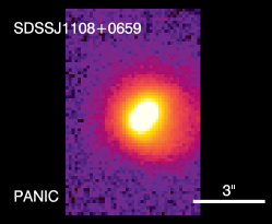
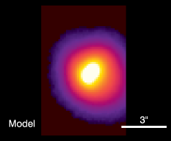
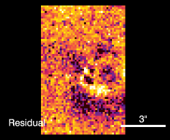
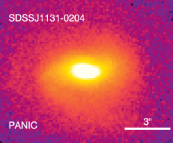
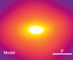
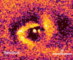
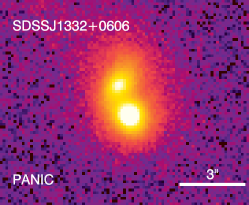
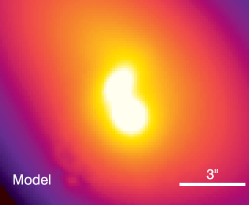
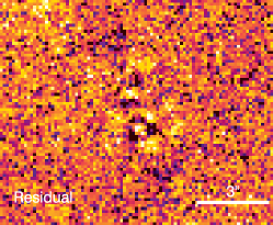
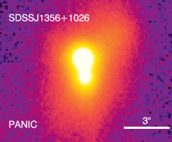
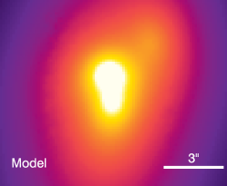
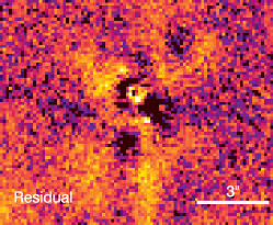
Figure 1: Model fits of the NIR surface brightness for four objects classified as binary AGNs (§3.1) using GALFIT. North is up and East is left. The first column shows the data, the second column shows the models and the last column shows the residuals. See the text in §3.1 for details regarding the model fits. Note that the residual maps have been re-stretched to enhance the contrast and the residuals are not important compared to the observed fluxes (the apparent excess in some of the residual maps has values less than $5\%$ of the observed fluxes at the corresponding locations).

Not all of these double-peaked [O III] objects are kpc-scale binary AGNs. Spatially resolved studies of nearby Seyferts frequently show a quite dynamic picture of the NLR, involving outflows, inflows, rotation, and interactions with a radio jet. Indeed, double-peaked [O III] features were already seen in early NLR studies (e.g., Sargent, 1972; Heckman et al., 1981; Veilleux, 1991). One famous example is Mrk 78, which has a bipolar outflowing NLR structure, broadly aligned with the linear radio jet (e.g., Whittle & Wilson, 2004; Whittle et al., 2005; Fischer et al., 2010); its spatially integrated spectrum shows a clear double-peaked [O III] line profile (see fig. 1 of Heckman et al., 1981). Spatially resolved studies with HST have revealed more such cases (such as NGC 1068 and NGC 4151, e.g., Crenshaw & Kraemer, 2000; Crenshaw et al., 2000; Veilleux et al., 2001; Das et al., 2005), where the NLR is dominated by outflows and/or rotation. For these dynamic NLRs, double-peaked features will naturally arise in spatially-integrated spectra when viewed at proper angles. Moreover, these outflows or rotating gaseous disks can extend as far as a few kpc. Thus detecting two [O III] peaks offset by a few kpc in slit spectra alone is not sufficient to conclude that the object is a kpc-scale binary AGN. All these complications simply reflect the diverse nature of NLR gas dynamics, and follow-up observations are needed to identify bona fide kpc-scale binary AGNs from the double-peaked [O III] sample.

To that end, we have been conducting follow-up observations of our double-peaked [O III] sample (Paper I) with ground-based NIR imaging and slit spectroscopy. The NIR imaging offers spatial resolution $\sim 0.6$″ (much better than the typical $\sim 1.4$″ seeing for optical SDSS imaging), and probes the old stellar populations (mostly stars in the bulge). Unlike the NLR gas, the stellar populations are unlikely to be involved in outflows, thus are a much less ambiguous indicator of the binary nature than using the NLR gas as a tracer. Slit spectroscopy probes the spatial distribution of NLR gas emission, giving the spatial information unavailable in the SDSS fiber spectra. Once a pair of nuclei are resolved in the NIR imaging, slit spectroscopy is required to associate the two [O III] peaks with each of the two nuclei. If, as is the case for Mrk 78, the NIR image shows a smooth stellar distribution while the optical spectrum shows two spatially offset [O III] peaks without NIR counterparts, then the double-peaked feature seen in the spatially integrated spectrum is more likely due to the kinematics of the NLR of a single AGN. Our imaging and spectroscopy follow-up observations have led to the discovery of several candidate binaries (Liu et al., 2010a). In these objects, we see spatially resolved double nuclei in the NIR images, whose locations are coincident with the two [O III] components in the slit spectra. The two [O III] components have a relative velocity offset of a few hundred ${\rm kms^{-1}}$, which leads to the double-peaked profile in the SDSS spectrum. The two components in each case have emission line flux ratios that place them in the AGN region of the BPT diagram (Baldwin et al., 1981). These cases strongly suggest that they are binary AGNs at $\sim$ kpc (projected) separations, which are co-rotating along with their stellar bulges and are ionizing their individual NLRs in a merging pair of galaxies.

Recently, the interest of these double-peaked [O III] objects has led to two NIR imaging studies with ground-based adaptive optics (AO) systems (Fu et al., 2010; Rosario et al., 2011). With diffraction-limited resolution ($\sim 0.1$″), these studies were able to resolve even closer double nucleus in the NIR than our imaging data under natural seeing. However, optical spectroscopy is still needed to register the resolved double nucleus with the [O III] emission in order to confirm the binary AGN nature, which becomes challenging on these smallest scales from the ground.

In this paper we present a summary of our imaging and spectroscopy follow-up for 31 objects in our parent sample of double-peaked [O III] type 2 AGNs presented in Paper I. The details of the parent sample (167 objects) can be found in that paper. Here we briefly describe the construction of this sample. We started from a sample of $\sim 15,000$ type 2 AGNs mostly from the MPA-JHU SDSS DR7 galaxy sample with the following criteria: (1) the rest-frame wavelength ranges [4700, 5100]Å and [4982, 5035]Å centered on the [O III] $\lambda$5007 line have median signal-to-noise ratio (S/N) $>5$ pixel^-1 and bad pixel fraction $<30\%$; (2) the [O III] $\lambda$5007 line is detected at $>5\sigma$ and has a rest-frame equivalent width (EW) $>4$Å; 3) the line flux ratio [O III] $\lambda$5007/H$\beta$$>3$ if $z>0.33$, or the diagnostic line ratios [O III] $\lambda$5007/H$\beta$and [N II] $\lambda$6584/H$\alpha$ lie above the theoretical upper limits for star-formation excitation from Kewley et al. (2001) on the BPT diagram (Baldwin et al. 1981) if $z<0.33$. All AGNs were then visually inspected and those with well-detected double peaks in both [O III] $\lambda$4959 and [O III] $\lambda$5007 with similar profiles were included in our final sample. We did not include those with complex line profiles such as lumpy, winged, or multi-component features.

The structure of the paper is as follows. We describe our observations and data reduction in §2, followed by discussions of individual objects in §3, where we categorize objects into binaries (§3.1), NLR kinematics around single AGNs (§3.2), and ambiguous cases (§3.3). We discuss the frequency of kpc-scale binary AGNs in §4, and conclude in §5. Throughout this paper we adopt a flat $\Lambda$CDM cosmology with $\Omega_{0}=0.3$, $\Omega_{\Lambda}=0.7$ and $H_{0}=70\,{\rm kms^{-1}Mpc^{-1}}$.

2 Observations and Data Reduction

2.1 NIR Imaging

We obtained $K_{s}$-band (or $J$-band if $K_{s}$ is unavailable) images for $61$ objects in our double-peaked sample during six nights in two observing runs using the Persson’s Auxiliary Nasmyth Infrared Camera (PANIC; Martini et al., 2004) on the 6.5 m Magellan I (Baade) telescope. Here we report 31 of these objects for which we also have slit spectroscopy, and will publish the remaining imaging data when slit spectroscopy data become available. The first observing run was on the nights of 2009 December 29 through 2010 January 2 UT and the second was on the night of 2010 May 30 UT. The typical observing procedure consisted of two sequences each dithered at nine positions with 25″ offsets. We obtained four 15-second exposures at each position so that the typical total exposure time per target was 18 min. We observed standard stars (Persson et al., 1998) at the beginning, middle, and end of each night. The observing conditions were clear but not photometric, with seeing ranging between 0″.5 and 0″.8 in the optical (through an RG610 filter) during the first run and 0″.7 and 1″.5 during the second. Table 1 lists total exposure times and seeing measured from field stars whenever available or from adjacent observations otherwise.

PANIC has a $2^{\prime}\times 2^{\prime}$ field of view (FOV) and 0″.125 pixels. We reduced PANIC data using the Carnegie Supernova Project pipeline (Hamuy et al., 2006) following standard procedures, including spatial-distortion correction, dark subtraction, bad-pixel masking, flat fielding (using twilight flats), sky subtraction, and aligning and stacking of the dithered frames. We determined $K_{s}$ and $J$ photometric zero points using 2MASS (Skrutskie et al., 2006) magnitudes of field stars when available, or the standard stars we observed during each night.

2.2 Optical Slit Spectroscopy

We conducted optical slit spectroscopy using the Low-Dispersion Survey Spectrograph (LDSS3) on the 6.5 m Magellan II (Clay) telescope and the Dual Imaging Spectrograph (DIS) on the Apache Point Observatory 3.5 m telescope. To date we have observed 31 objects with NIR imaging data. All objects which appear to have double nuclei in their NIR images were observed with slit spectroscopy.

Our LDSS3 runs were on the nights of 2010 January 12 through 14 UT. The observing conditions were clear but not photometric, with seeing ranging between 0″.7 and 1″.1. LDSS3 has a 8^′.3 diameter FOV and 0″.188 pixels. We employed a 1${}^{\prime\prime}\times$4^′ long-slit with the VPH-Blue grism to cover H$\beta$ and [O III] in the blue ($\sim$ 4260–7020Å), and the VPH-Red grism (with the OG590 filter) to cover H$\alpha$ and [N II] in the red ($\sim$ 5800–9800Å). The spectral resolution was 3.1 (6.3) Å FWHM in the blue (red). For most of our LDSS3 targets we only obtained spectra in the blue due to observing time constraints. For objects with double stellar components identified either from our NIR imaging or from SDSS images, we oriented the slit to go through the two stellar components; for the others we oriented the slit along the major axis of the galaxy. For a few targets whose [O III] emission along the primary slit position was either not spatially resolved or was particularly complex, we obtained spectra at a second slit position usually perpendicular to the primary slit position. We list slit positions, total exposure times, and seeing measured from field stars in acquisition images in Table 1. We took wavelength calibration spectra and flat fields after observing each object. During the course of each night, we observed two white dwarfs at different airmasses for spectrophotometric calibration and several K and M giants for velocity calibration.

Our DIS observations were carried out during eight nights between 2009 July 15 and 2010 July 14 UT. The observing conditions were partly cloudy or clear but not photometric on the nights of 2009 July 15, September 23, December 12 and 19, and 2010 July 07 and 14, and photometric on the nights of 2010 February 15 and June 10 UT. During most nights the seeing was poor, ranging between 1″.5 and 2″.7 (except the nights of 2009 December 12 and 19 with seeing around 1″.0). DIS has a 4${}^{\prime}\times$6^′ FOV and 0″.414 pixels. The spectral resolution was 1.8 (1.3) Å FWHM in the blue (red) channel. We adopted a 1″.5$\times$6^′ slit and the B1200+R1200 gratings centered at 5000 and 7000 Å (or 5200 and 7050 or 5500 and 7450 or 5550 and 7550 Å, depending on target redshifts). The slit orientation was determined in the same way as in our LDSS3 runs.

We reduced the LDSS3 and DIS data following standard IRAF procedures (Tody, 1986) and with the COSMOS reduction pipeline. The 2d data reduction included bias subtraction, flat fielding, cosmic ray removal, wavelength calibration and spatial rectification, flux calibration and extinction correction, sky subtraction, and aligning and stacking of individual frames. We applied telluric correction over the extracted 1d spectra using standard stars; the O₂ A-band (7580–7740Å) is the major feature that affects the region of interest in the red. The quality of the LDSS3 data is substantially better than that of the DIS data due to the much better seeing and larger telescope, hence we will always present LDSS3 data whenever available.

Table 1: Observing Summary

	NIR Imaging				Slit Spectroscopy
SDSS Name	Instrument	Seeing	Obs Date	Exp Time	Instrument	Seeing	Obs Date	PA	Exp Time
		(″)	UT	(min)		(″)	UT	(∘)	(sec)
0002$+$0045	PANIC $K_{s}$	0.48	091230	9	DIS	1.1	091212	71	1800
0009$-$0036	PANIC $K_{s}$	0.63	091231	18	LDSS3	0.94	100113	278	900
0116$-$1025	PANIC $K_{s}$	0.52	091229	18	LDSS3	0.83	100112	95	1800
0135$-$0058	PANIC $K_{s}$	0.58	091229	18	LDSS3	0.86	100112	101	1800
0135$+$1435	PANIC $J$	0.55	100101	18	LDSS3	0.92	100113	200	900
0156$-$0007	PANIC $K_{s}$	0.64	091229	18	LDSS3	1.0	100113	299	1800
0400$-$0652	PANIC $K_{s}$	0.48	091229	18	LDSS3	0.58/0.57	100112/100114	95/173	2700/1800
0837$+$1500	PANIC $K_{s}$	0.66	091229	27	LDSS3	1.1	100113	322	1800
0851$+$1327	PANIC $K_{s}$	0.49	091230	18	LDSS3	0.91	100114	201	900
0942$+$1254	PANIC $K_{s}$	0.50	091229/100102	36	LDSS3	0.88/0.95	100112/100113	213/348	2700/1800
0958$-$0051	PANIC $K_{s}$	0.45	091230	18	LDSS3	0.87	100113	200	900
1009$+$0133	PANIC $K_{s}$	0.44	091230	18	LDSS3	0.84	100114	217	900
1019$+$0134	PANIC $K_{s}$	0.70	091229	18	LDSS3	0.94	100114	303	900
1038$+$0255	PANIC $K_{s}$	0.45	091231	18	LDSS3	0.75	100114	270	900
1108$+$0659	PANIC $K_{s}$	0.54	091229	18	LDSS3	0.86/0.95	100112/100113	320	4800
1131$-$0204	PANIC $K_{s}$	0.47	091231/100102	36	LDSS3	0.94/0.71	100112/100113	267	2700/3600
1146$-$0226	PANIC $K_{s}$	0.64	100102	18	LDSS3	0.98	100114	233†	900
1146$+$5110	2MASS $K$	…	…	…	DIS	1.7	100215	51	4800
1322$+$2631	PANIC $K_{s}$	0.73	100530	18	DIS	2.0/1.8	100707/100714	79	1800/3600
1332$+$0606	PANIC $J$	0.52	100101	18	LDSS3	1.2/0.86	100112/100114	196	2400/2100
1341$+$2219	PANIC $K_{s}$	0.74	100530	18	DIS	1.4	100707	175	3600
1356$+$1026	PANIC $K_{s}$	0.79	100530	18	LDSS3∗	…	…	…	…
1450$+$0838	PANIC $K_{s}$	0.85	100530	18	DIS	2.4/2.5	100707/100714	55	3600/1800
1552$+$0433	PANIC $K_{s}$	0.71	100530	18	DIS	1.3	100610	303	3600
1556$+$0948	PANIC $K_{s}$	0.58	100530	18	DIS	1.5	100610	158	3000
1630$+$1649	PANIC $K_{s}$	0.86	100530	18	DIS	1.6	100610	39	3000
2252$+$0029	PANIC $K_{s}$	0.83	100530	27	DIS	1.5	091219	162	2400
2255$-$0812	PANIC $K_{s}$	0.86	100530	18	DIS	1.5	091219	180	2400
2304$-$0933	PANIC $K_{s}$	0.80	100530	18	DIS	2.0	090923	61	1800
2310$-$0900	PANIC $K_{s}$	0.62	091230	18	DIS	2.0	090923	73	2700
2333$+$0049	PANIC $K_{s}$	0.76	091229	18	DIS	1.5	091219	117	3600

Note. — Summary of our NIR imaging and optical slit spectroscopy observations. The full SDSS designations are given in Table 2. For some objects we have two observations, which are listed separately. ^†Parallactic angle. ^∗The spectroscopic observation was reported in Greene et al. (2011).

Table 2: Object Properties

SDSS Name	redshift	PANIC offset ″ (kpc)	Spec offset ″ (kpc)	Category
000249.07$+$004504.8	0.0868		0.8 (1.3)	NLR kinematics
000911.58$-$003654.7	0.0733		$<0.2$ ($<0.3$)	ambiguous
011659.59$-$102539.1	0.1503		0.9 (2.3)	NLR kinematics
013546.93$-$005858.5	0.1595		0.2 (0.6)	NLR kinematics
013555.82$+$143529.7	0.0719		0.8 (1.1)	NLR kinematics
015605.14$-$000721.7	0.0806		0.6 (0.9)	NLR kinematics
040001.59$-$065254.1	0.1707		1.3/$<0.2$ (3.8/$<0.6$)	NLR kinematics
083713.49$+$150037.2	0.1408		1.3 (3.2)	NLR kinematics
085121.94$+$132702.2	0.0931		0.6 (1.0)	NLR kinematics
094205.83$+$125433.7	0.1543		0.2/$<0.2$ (0.5/$<0.5$)	ambiguous
095833.20$-$005118.6	0.0860		0.8 (1.3)	NLR kinematics
100921.26$+$013334.6	0.1437		0.2 (0.5)	ambiguous
101927.56$+$013422.5	0.0730		0.3 (0.4)	ambiguous
103850.13$+$025555.1	0.0762		0.9 (1.3)	NLR kinematics
110851.04$+$065901.4	0.1816	0.5 (1.5)	0.9 (2.7)	binary AGNa
113126.08$-$020459.2	0.1463	0.6 (1.5)	0.6 (1.5)	binary AGNa
114610.04$-$022619.2	0.1225		1.3 (2.9)	NLR kinematics
114642.47$+$511029.6	0.1300	2.7 (6.2)	2.5 (5.8)	binary AGNa
132231.86$+$263159.1	0.1441		2.1 (5.3)	ambiguous
133226.34$+$060627.4	0.2070	1.5 (5.1)	1.5 (5.1)	binary AGNa
134114.87$+$221957.8	0.1152		1.7 (3.5)	NLR kinematics
135646.11$+$102609.1	0.1231	1.3 (2.9)	1.3 (2.9)b	binary AGNb
145050.60$+$083832.6	0.1168		$<0.4$ ($<0.8$)	ambiguous
155205.93$+$043317.5	0.0803		1.2 (1.8)	NLR kinematics
155619.30$+$094855.6	0.0678		0.4 (0.5)	ambiguous
163056.75$+$164957.2	0.0341		0.8 (0.5)	NLR kinematics
225252.94$+$002928.4	0.1525		$<0.4$ ($<1.1$)	ambiguous
225510.12$-$081234.4	0.1494		0.4 (1.0)	ambiguous
230442.82$-$093345.3	0.0319		0.8 (0.5)	NLR kinematics
231051.95$-$090011.9	0.0944		$<0.4$ ($<0.7$)	ambiguous
233313.17$+$004911.8	0.1699		$<0.4$ ($<1.2$)	ambiguous

Note. — Properties of the 31 objects in our sample. In those cases which showed two nuclei in NIR imaging, column 3 shows the spatial offset (in units of ″ and kpc) between the two nuclei, which is measured from the emission peaks of the two nuclei. Column 4 shows the spatial offset (in units of ″ and kpc) between the two velocity components of the narrow line emission, measured from the emission peaks of the two velocity components in the slit spectrum. The smallest spatial offset of the two velocity components we can measure is the pixel scale, i.e., $\sim 0.2$″ for LDSS3 and $\sim 0.4$″ for DIS. For J0400-0652 and J0942+1254 we have measurements for two slit position angles. The last column shows our classification of these objects (see §3). ^aPublished in Liu et al. (2010a); ^bSlit spectrum reported in Greene et al. (2011).

3 Interpretation

Our combined NIR imaging and slit spectroscopy data reveal that double-peaked [O III] emission arises from a diverse set of circumstances. We classify them by examining the NIR images and the two-dimensional spectra simultaneously. Given the typical seeing conditions in our NIR imaging, two stellar components with $K_{s}$ luminosities that are within an order of magnitude of each other can be identified at separations $\gtrsim 0.6$″. The seeing is poorer in our optical slit spectroscopy. However, the two [O III] components are spectrally resolved, which makes it easier to deblend them spatially in the 2d spectrum. We measure the spatial offset between the peak emission of the two velocity components in the 2d spectra (Table 2), which can be measured down to one pixel scale ($0.188$″ for LDSS3 and 0.414″ for DIS).

Based on the NIR imaging and slit spectroscopy data, we classify the 31 objects in three categories (Table 2):

1. Kpc-scale binary AGNs: There are two spatially resolved (or marginally resolved) stellar nuclei in NIR imaging. The two velocity components of the narrow line emission are spatially coincident with the pair of nuclei seen in the NIR. These are the best candidates for kpc-scale binary AGNs in our sample. Five objects are included in this category, four of which were reported in Liu et al. (2010a).

2. NLR kinematics in single AGNs. The NIR imaging shows a single smooth stellar component, but the two velocity components of the narrow lines are spatially offset by $\gtrsim 0.6$″. We performed tests with simulated images of two stellar components with different luminosity contrasts, structural parameters and seeing conditions, and concluded that two stellar components with comparable ($0.1\lesssim L_{1}/L_{2}\lesssim 10$) luminosities under the actual seeing would have been resolved in NIR imaging at the separation indicated by the two [O III] components. There could still be two stellar components hidden in the system if, e.g., the luminosity contrast is larger than an order of magnitude, the separation of the two stellar components is smaller than that inferred from the narrow line emission, or one of the stellar components has an unusual surface brightness profile. But given the similar appearances of these objects in NIR imaging and slit spectroscopy to the classic example of Mrk 78 (see §1), the simplest explanation is that the double peaks emerge from multiple kinematic components in a single NLR for the majority of these sources. Fifteen objects are included in this category. We refer to these objects below as having NLR kinematics origin.

3. Ambiguous cases. For the remaining objects, a single nucleus is seen in the NIR imaging, and the two velocity components of the narrow lines are spatially offset by $\lesssim 0.4$″, smaller than the resolution of our NIR imaging. These objects could be single AGNs with NLR structure on smaller scales, or binary AGNs at smaller separations. We need better spatial-resolution observations and/or different slit positions to test these scenarios. Eleven objects are included in this category.

These three categories represent our best effort to interpret these objects based on current data; they are by no means exact. In particular, the binary AGN and NLR kinematics classifications both have caveats that may cause us to misinterpret their nature. Keeping this in mind, we adopt this classification scheme in our following discussion. Below we summarize the objects in each category, and discuss the caveats.

3.1 Kpc-Scale Binary AGNs

Our primary interest is to identify bona fide kpc-scale binary AGNs, which motivated our original search for these double-peaked objects in SDSS spectroscopic database. Most of our NIR imaging preceded the slit spectroscopy, and we obtained spectra of all our targets with resolved double nuclei in the NIR. Five out of $\sim 60$, or $\sim 10\%$ of our objects show resolved double stellar nuclei in their NIR images. Their two-dimensional (2d) spectra show that the two [O III] velocity components seen in the spatially-integrated spectra are spatially coincident with the two stellar continuum peaks.

For the sky-subtracted NIR imaging data, we use GALFIT (Peng et al., 2010) to model the light distribution with multiple components. PSFs were taken from stars within the same image. Due to the complexity of merging systems, and the fact that the results depend on the quality of the data, we only use the exponential disk (expdisk), de Vaucouleurs (devauc) and Sérsic (sersic) profiles in each fits, and we urge caution on the interpretation of the best-fit model for some of these objects. During the fits we did not fix any of the model parameters, and for each fit we tried different combinations of the above three profiles until it reaches the minimum reduced $\chi^{2}$. Fig. 1 shows the best-fit model (and the residuals) along with data for the four objects with PANIC data. The best-fit models are summarized in Table 3, where the best-fit parameters have been rounded using the 1$\sigma$ statistical uncertainties from GALFIT. Due to the nature of nonlinear multi-component models and possible systematic effects involved in the data (such as bad PSF or sky subtraction), the statistical uncertainties reported by GALFIT are an approximation of the actual uncertainties at best. We use these model fits to estimate the luminosity ratios of multiple stellar components in these merging systems, and to determine the galaxy type of each component.

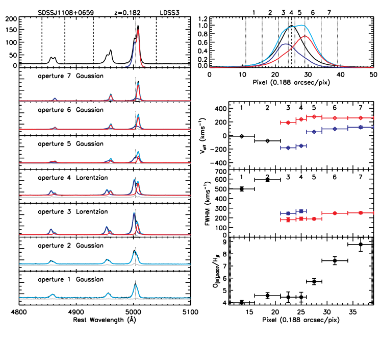
Figure 3: Diagnosis of the 2d spectrum of J1108+0659. The left panel shows the 1d spectra summed over the entire slit (uppermost) and for slit slices at 7 different spatial locations (flux scale is arbitrary). The dotted vertical lines divide the [O III] $\lambda$5007 line into the blueshifted and redshifted components. The dashed vertical lines separate the emission line regions from the continuum regions. The upper-right panel shows the spatial profiles of the continuum (black) and the [O III] $\lambda$5007 emission line region (cyan), while the blue and red lines show the spatial profile of the blueshifted and redshifted [O III] $\lambda$5007 emission. We slice the 2d spectra in seven spatial bins (marked by the numbers), centered on the spatial peak of the continuum emission, and the 1d spectra for these spatial bins are shown in the left panel. For the 1d spectrum in each spatial bin, we try to deblend the two velocity components in the emission lines by fitting the spectrum with double Gaussian/Lorentzian functions and a local continuum model. We consider the deblending successful if the two components have a flux ratio greater than 0.3 and both components were detected at $>3\sigma$. If the deblending is successful we over-plot the two velocity components in blue and red respectively in the aperture spectra, otherwise we over-plot the whole model in cyan. We plot the velocity offset (relative to the systemic redshift) and FWHM of the two components, and the [O III] $\lambda$5007/H$\beta$ flux ratio measured from the model in the bottom-right panels. In a few cases the apparent “successful” deblending in a spatial bin can still be spurious as judged by eye; we nevertheless plot results for these bins, but such bins should be ignored in assessing the spatial gradients of these quantities.

For the slit spectra, we extract one-dimensional (1d) spectra at different spatial locations along the slit. We model the 1d spectra in different spatial bins with double-Gaussian (or double-Lorentzian if a better fit can be achieved) profiles for the double-peaked lines, plus a power-law model for the local continuum. Fig. 3 shows an example of the results of our modeling. Our goal is to see if there are observable trends in the velocity, line width, and line flux ratio of the two narrow line components. Unfortunately, given the typical seeing in our slit spectroscopy, these trends are only apparent in a few cases. There are several objects for which the spectral quality is too poor to perform such analysis. Below we briefly comment on individual objects.

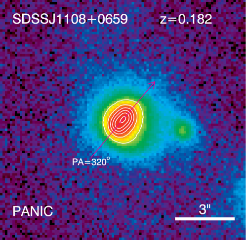
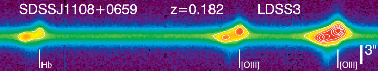
Figure 2: SDSS J1108+0659 (binary). Top: PANIC NIR image in $K_{s}$. North is up and East is left. The magenta line shows the direction of the slit used in the spectroscopy, with the arrow indicating the upper direction in the extracted 2d spectrum. This object has two (marginally) resolved stellar nuclei separated by $\sim 0.5$″ in the cental galaxy. There is also a faint companion to the right which is not covered by the slit spectrum. Bottom: LDSS3 2d spectrum for the H$\beta$-[O III] region with corresponding lines marked (note that the locations of these line marks are approximate). The two velocity components are spatially offset by 0.9″. The stellar continua are not separated in the 2d spectrum due to the limited seeing and the proximity of the two stellar nuclei.

J1108+0659. This object was reported in Liu et al. (2010a). It shows two nuclei in its NIR image, separated by $\sim 0.5$″. The two [O III] velocity components are spatially coincident with the two NIR nuclei. Its $K_{s}$-band image and 2d spectrum for the [O III]-H$\beta$ region are shown in Fig. 2. The pair of nuclei are well resolved in a recent NIR adaptive-optics (AO) imaging observation (Fu et al., 2010). The best-fit $K_{s}$-band model consists of two de Vaucouleurs bulges embedded in an exponential disk. The luminosity contrast of the two bulges is $\sim 0.15$ magnitude (0.06 dex).

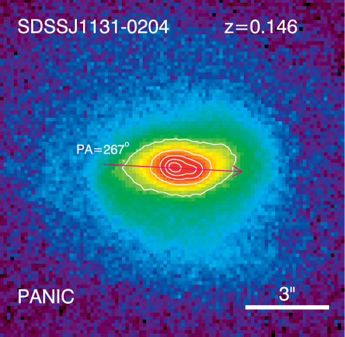
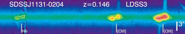
Figure 4: SDSS J1131$-$0204 (binary). Upper: PANIC NIR image in $K_{s}$. This object has two stellar nuclei separated by $\sim 0.6$″. Bottom: LDSS3 2d spectrum for the H$\beta$-[O III] region with corresponding lines marked (note that the locations of these line marks are approximate). The two velocity components are spatially offset by $\sim 0.6$″. Notation is the same as Fig. 2. For this object, the two stellar nuclei are embedded in a disk, and the long “spur” features seen in the 2d spectrum are from ionized gas emission in the disk.

J1131$-$0204. This object was reported in Liu et al. (2010a). It shows two resolved stellar nuclei separated by $\sim 0.6$″. The slit spectroscopy confirmed the coincidence of the two [O III] velocity components with the two NIR nuclei. Its $K_{s}$-band image and 2d spectrum for the [O III]-H$\beta$ region are shown in Fig. 4. The two stellar nuclei are embedded within a galactic disk, and the long “spur” features seen in the 2d spectrum to $>15$ kpc are ionized gas emission from the disk which traces the galactic rotation curve. The best-fit $K_{s}$-band model consists of one Sérsic bulge ($n\approx 3$) and one de Vaucouleurs bulge embedded in an exponential disk. The luminosity contrast of the two bulges is $\sim 2$ magnitude (0.8 dex). The model fit is imperfect and there is some residual spiral structure indicative of interactions.

J1146+5110. This object was reported in Liu et al. (2010a). The double stellar nuclei were marginally resolved in the 2MASS $K_{s}$ image, and our slit spectroscopy subsequently confirmed the coincidence of the two [O III] velocity components with the two NIR nuclei. This is also one of the few cases that show resolved optical double nuclei in the SDSS images. The southern nucleus itself seems to have a complex NLR geometry and two NLR velocity components. The double nucleus was well resolved in the NIR AO imaging in Fu et al. (2010), with a luminosity contract of 0.7 magnitude (0.28 dex). We do not have a PANIC image for this object.

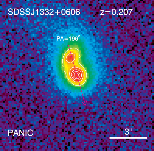
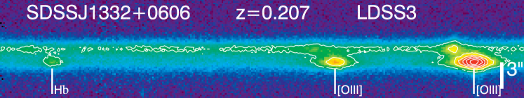
Figure 7: SDSS J1332+0606 (binary). Upper: PANIC NIR image in $J$. This object has two stellar nuclei separated by $\sim 1.5$″. Bottom: LDSS3 2d spectrum for the H$\beta$-[O III] region with corresponding lines marked (note that the locations of these line marks are approximate). The two velocity components are spatially offset by $\sim 1.5$″. Notation is the same as Fig. 2. The two continua are also separated in the 2d spectrum. The northern nucleus with the weaker continuum has stronger [O III] emission.

J1332+0606. This object was reported in Liu et al. (2010a). The two stellar nuclei were clearly resolved in optical (SDSS) and $J$-band images, and are spatially coincident with the two [O III] velocity components seen in our slit spectroscopy. Its $J$-band image and 2d spectrum for the [O III]-H$\beta$ region are shown in Fig. 7. The best-fit $J$-band model consists of three components: a Sérsic bulge ($n\approx 2$) for the southern nucleus, an exponential disk for the northern nucleus, and an exponential disk with a scale-length of $r_{s}\sim 1.6$″. The luminosity ratio of the three components is $\sim 2:1:1$. The less luminous northern stellar component corresponds to the stronger [O III] emission component seen in the slit spectrum, as in J1322+2631.

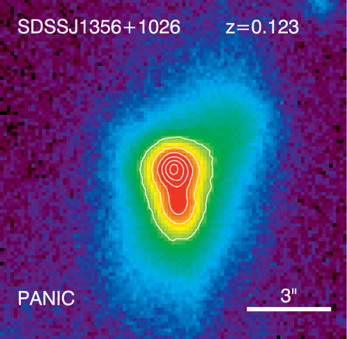
Figure 9: SDSS J1356+1026 (binary). Upper: PANIC NIR image in $K_{s}$. This object has two stellar nuclei separated by $\sim 1.3$″. It shows a highly disturbed morphology, presumably caused by the merger. The slit spectroscopy of this object was reported in Greene et al. (2011).

J1356+1026. This object was studied in Greene et al. (2011). It shows two continuum sources in the optical separated by $\sim 3$ kpc, corresponding to the north and south knots of [O III] emission seen in the slit spectrum in Greene et al. (2011). The two knots of [O III] emission have a relative velocity offset of $\sim 200\ {\rm km\,s^{-1}}$. The slit spectrum in Greene et al. (2011) shows a rich [O III] emission structure, including a giant [O III] bubble to the South of the southern continuum. Its $K_{s}$-band image is shown in Fig. 9. This is a galaxy with a highly disturbed morphology and its IRAS fluxes indicate that it is a ULIRG. The best-fit $K_{s}$-band model consists of three components: a Sérsic bulge ($n\approx 5$) for the southern nucleus, a Sérsic bulge ($n\approx 3$) for the northern nucleus, and an exponential disk component ($r_{s}\sim 0.8$″) towards the north-western corner. The luminosity ratio of the three components is $\sim 15:5:1$. However, due to the highly disturbed morphology of this system, we urge caution on the best-fit model. This object was also observed with NIR AO imaging in Fu et al. (2010).

Table 3: Model fits of NIR images

Object	$n_{s}$	$R_{e}/r_{s}$	$(x_{c},y_{c})$	$q$	PA	Mag
		(pixel/kpc)	(pixel)		(∘)	(Vega)
J1108+0659 ($K_{s}$)			$\chi^{2}_{\nu}=0.19$
devauc (S)	4	3.2/1.2	$(94.1,99.8)$	0.60	46	15.46
devauc (N)	4	3.2/1.2	$(97.3,103.6)$	0.61	$-$42	15.32
expdisk	1	8.5/3.2	$(101.4,99.8)$	0.80	46	15.70
J1131$-$0204 ($K_{s}$)			$\chi^{2}_{\nu}=1.00$
sersic (E)	3.2	25.2/8.1	$(98.1,101.6)$	0.46	$-$88	15.12
devauc (W)	4	14.8/4.7	$(104.2,100.3)$	0.28	$-$69	17.24
expdisk	1	22.2/7.1	$(101.5,97.9)$	0.71	13	15.67
J1332+0606 ($J$)			$\chi^{2}_{\nu}=1.08$
expdisk (N)	1	3.0/1.3	$(98.2,107.6)$	0.53	$-$33	17.92
sersic (S)	2.0	4.4/1.9	$(102.2,96.4)$	0.85	27	17.06
expdisk	1	13.1/5.5	$(100.1,115.9)$	0.55	46	17.79
J1356+1026∗ ($K_{s}$)			$\chi^{2}_{\nu}=0.91$
sersic (N)	3.2	4.6/1.3	$(99.0,108.0)$	0.79	$-$80	15.55
sersic (S)	5.6	63.1/17.4	$(100.2,97.4)$	0.53	$-$8	14.34
expdisk	1	6.7/1.9	$(115.6,121.2)$	0.67	$-$1	17.32

Note. — Best-fit surface brightness models for four objects that show multiple stellar components in the NIR. Only the Sérsic (including de Vaucouleurs) and the exponential disk profiles were used in these fits. We report best-fit parameters for the Sérsic index ($n$), the effective radius ($R_{e}$) or scale-length ($r_{s}$), the centroid of each component ($x_{c},y_{c}$), the aspect ratio ($q$), the position angle of the major axis (PA), and the integrated magnitude for each component (normalized using the total 2MASS flux). These parameters are rounded using the statistical errors from the fits. Due to the complexity of these systems, we caution that a “successful” model may not be the unique model, and the actual errors of these parameters are expected to be substantially larger. This is especially a concern for J1356 (marked with a “*”), whose morphology is quite disturbed. We report scales in units of pixels, where 1 pixel corresponds to 0.125″.

All of these objects appear to be major mergers (the $K_{s}$-band luminosity ratio between the two main stellar components is less than 10), which is partly due to our selection based on comparable [O III] luminosities. But we also note that the more massive stellar component does not necessarily have stronger [O III] emission.

We classify these objects as kpc-scale binary AGNs based on spatially coincident double stellar nuclei and [O III] emission. While the binary scenario seems to be the most natural explanation, it is possible that only one SMBH is active and ionizing the gas clouds in both nuclei. In this single-AGN scenario, the [O III] gas clouds in the non-AGN host are further away from the ionizing source than those in the AGN host. This difference will lead to different ionization states in the [O III] clouds in the two hosts. If we assume that the electron density is similar in both hosts, we expect very different [O III]/H$\beta$ flux ratios of the two narrow line components, contrary to what we observe (Liu et al., 2010a). However, the electron density may well be quite different in the two hosts, allowing a single AGN within one host to be responsible for the [O III] emission in both hosts. This is particularly relevant for the ULIRG J1356+1026, where the interstellar medium (ISM) may be quite clumpy. Our current data are insufficient to completely rule out the single AGN possibility. We are currently acquiring images with HST and Chandra, as well as higher S/N slit spectroscopy for these objects, and further investigations of these objects will be presented in future work.

3.2 NLR Kinematics in Single AGNs

The remaining ($\sim 90\%$) objects with NIR imaging data do not show resolved (or marginally resolved) double nuclei at the limit of our resolution ($\sim 0.6$″). These unresolved cases fall into one of the following categories: a) they are binaries at smaller projected separations; b) they are two accreting BHs each with its own NLR, co-rotating within a single merged stellar bulge, or c) they are single AGNs with complex NLR kinematics.

About $60\%$ of the objects that appear single in the NIR imaging show spatially resolved [O III] emission (typically $\gtrsim 0.6$″) in the 2d spectra, which correspond to the two velocity components seen in the spatially-integrated spectra. Double stellar nuclei separated on these scales would have been identified in our NIR imaging. Thus the lack of spatially coincident stellar nuclei favors either scenario (b) or scenario (c). However, the NLR dynamics are presumably affected by the bulge potential more than by the BH, thus it is difficult to maintain two distinct NLRs in scenario (b). On the other hand, NLR kinematics involving rotation or outflows on sub-kpc to kpc scales are quite common for local Seyferts (see §1). In fact, in some of the objects with good spatial quality we can see velocity/velocity dispersion gradients along the slit direction in the 2d spectrum (see below), which strongly supports the kinematics scenario. Therefore we believe that the double velocity peaks in the vast majority of these objects arise from complex kinematics in a single NLR . We now comment on each of these objects in detail.

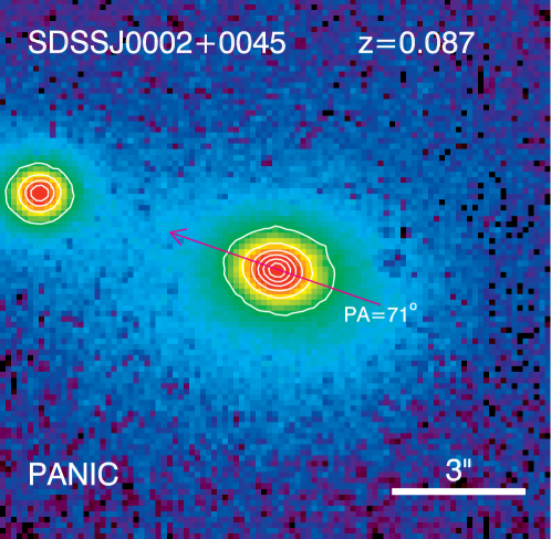
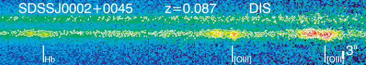
Figure 10: SDSS J0002+0045 (NLR kinematics). Upper: PANIC NIR image in $K_{s}$. This object shows a single nucleus, and has a companion $\sim 5$″ away toward the north-east (which is not covered by the SDSS fiber). Bottom: DIS 2d spectrum for the H$\beta$-[O III] region with corresponding lines marked (note that the locations of these line marks are approximate). The two velocity components are spatially offset by $\sim 0.8$″. The north-east companion does not have detectable [O III] emission. Notation is the same as Fig. 2.

J0002+0045. For this object the two velocity components of [O III] are spatially offset by $\sim 0.8$″, but they do not have a corresponding pair of nuclei seen in the NIR image. Fig. 10 shows the $K_{s}$ image and the 2d spectrum. Note that this object has a north-east companion $\sim 5$″ away, which does not have [O III] emission; this companion galaxy is at the same redshift as J0002+0045 measured from stellar absorption features in the slit spectrum.

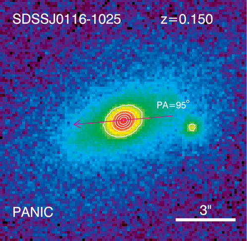
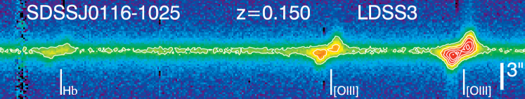
Figure 11: SDSS J0116-1025 (NLR kinematics). Upper: PANIC NIR image in $K_{s}$. This object has no resolved double nucleus, and it has a small companion $\sim 4$″ away towards the west (which is not covered by the SDSS fiber). Bottom: LDSS3 2d spectrum for the H$\beta$-[O III] region with corresponding lines marked (note that the locations of these line marks are approximate). The two velocity components are spatially offset by $\sim 0.9$″. Notation is the same as Fig. 2.

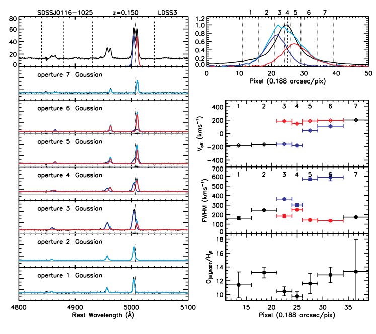
Figure 12: Diagnosis of the 2d spectrum of J0116$-$1025. Notation is the same as Fig. 3. The [O III]/H$\beta$ flux ratio is almost independent of position (within $\sim 0.15$ dex), but the [O III] line width seems to increase towards the center of the continuum emission except for the blueshifted component in bins 5 and 6. No obvious velocity gradient is seen for either of the two [O III] components, and the data are consistent with a flat rotation curve with $V_{c}\sin i\sim 200\ {\rm km\,s^{-1}}$ on each side of the continuum.

J0116$-$1025. This object has two spatially offset [O III] emission peaks, which correspond to the blue- and red-shifted components in the double-peaked line profile respectively. The spatial offset of the two [O III] components is $\sim 1.1$″, and there is no corresponding double nucleus seen in the NIR image. Fig. 11 shows the $K_{s}$ image and the 2d spectrum. The host galaxy clearly has a disk component. There is also a small galaxy about $\sim 4$″ away from the center of J0116-1025 to the West, which was not covered by our slit observation. Fig. 12 shows the 1d slices of the 2d spectrum at different distances from the peak of the continuum emission. The [O III] $\lambda$5007/H$\beta$ flux ratio is almost independent of position, but the [O III] line width increases towards the center of the continuum emission. No obvious velocity gradient is seen for either of the two [O III] components. Combining the NIR imaging and slit spectroscopic data, this object is best explained by a rotational [O III] disk co-planar with the stellar disk.

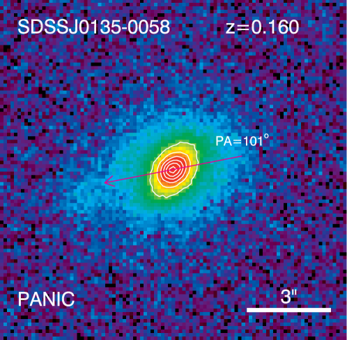
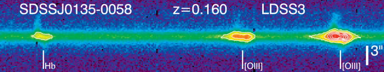
Figure 13: SDSS J0135$-$0058 (NLR kinematics). Upper: PANIC NIR image in $K_{s}$. This object has no resolved double nucleus. There are tidal features towards the south-east, which is covered by our slit observation. Bottom: LDSS3 2d spectrum for the H$\beta$-[O III] region with corresponding lines marked (note that the locations of these line marks are approximate). The two velocity components are spatially offset by $\sim 0.2$″. Notation is the same as Fig. 2.

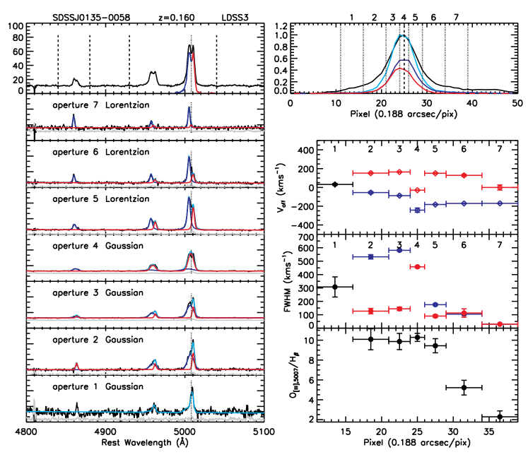
Figure 14: Diagnosis of the 2d spectrum of J0135$-$0058. Notation is the same as Fig. 3. The [O III]/H$\beta$ flux ratio is almost constant until the outermost apertures (6 and 7), where it drops rapidly as it is now tracing the faint tidal feature seen in the 2d spectrum. There is a slight velocity gradient for the blue- and red-shifted components. Deblending of the emission lines is ambiguous in bins 3 and 4.

J0135$-$0058. Fig. 13 shows the $K_{s}$ image and the 2d spectrum for this object. The long slit was placed to cover the tidal feature to the south-east of the galaxy seen in the NIR image, and hence was misaligned with the major axis of the disk. Fig. 14 shows the 1d slices of the 2d spectrum at different distances from the peak of the continuum emission. The [O III] $\lambda$5007/H$\beta$ flux ratio is almost constant until the outermost apertures (6 and 7), where the [O III] $\lambda$5007/H$\beta$ decreases as it is now tracing the faint tidal feature seen from the 2d spectrum shown in Fig. 13. There is a slight velocity gradient for the blue- and red-shifted components. Although the spatial offset between the two [O III] components is only $\sim 0.2$″ (possibly due to the misaligned slit position angle), we believe a rotational [O III] disk is the best explanation given the velocity gradient seen in the 2d spectrum as well as the apparent disk morphology seen in the NIR.

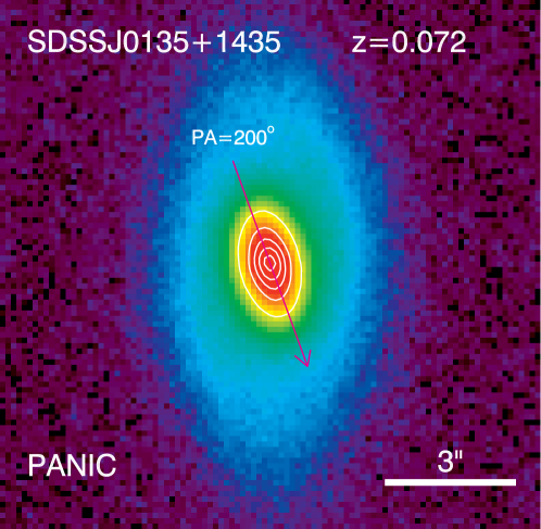
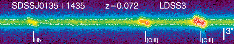
Figure 15: SDSS J0135+1435 (NLR kinematics). Upper: PANIC NIR image in $K_{s}$. This object has no resolved double nucleus. Bottom: LDSS3 2d spectrum for the H$\beta$-[O III] region with corresponding lines marked (note that the locations of these line marks are approximate). The two velocity components are spatially offset by $\sim 0.8$″. Velocity gradients can be seen in the 2d spectrum. Notation is the same as Fig. 2.

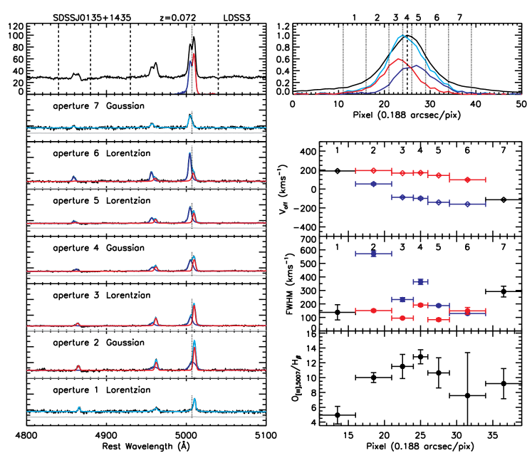
Figure 16: Diagnosis of the 2d spectrum of J0135+1435. Notation is the same as Fig. 3. We detect clear velocity gradients for the blueshifted and redshifted velocity components, and possible increasing velocity dispersion towards the center of the continuum. The [O III]/H$\beta$ flux ratio also increases towards the center of the continuum in general.

J0135+1435. Fig. 15 shows the $K_{s}$ image and the 2d spectrum for this object. The two velocity components of [O III] are spatially offset by $\sim 0.8$″, while no corresponding pair of nuclei was seen in the NIR. Fig. 16 shows the 1d slices of the 2d spectrum at different distances from the peak of the continuum emission. The [O III] $\lambda$5007/H$\beta$ flux ratio increases towards the center of the continuum emission. Velocity gradients for both [O III] components are clearly seen in Fig. 16, and there is some indication of increasing line width toward the center of the continuum emission, although decomposition into two components is not always successful at each aperture. This object is best explained by a rotational [O III] disk, with an asymptotic flat rotation velocity $V_{c}\sin i\sim 200\,{\rm kms^{-1}}$.

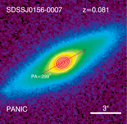
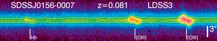
Figure 17: SDSS J0156$-$0007 (NLR kinematics). Upper: PANIC NIR image in $K_{s}$. This object has a single nucleus, and it has a large disk component. Bottom: LDSS3 2d spectrum for the H$\beta$-[O III] region with corresponding lines marked (note that the locations of these line marks are approximate). The two velocity components are spatially offset by $\sim 0.6$″. Notation is the same as Fig. 2.

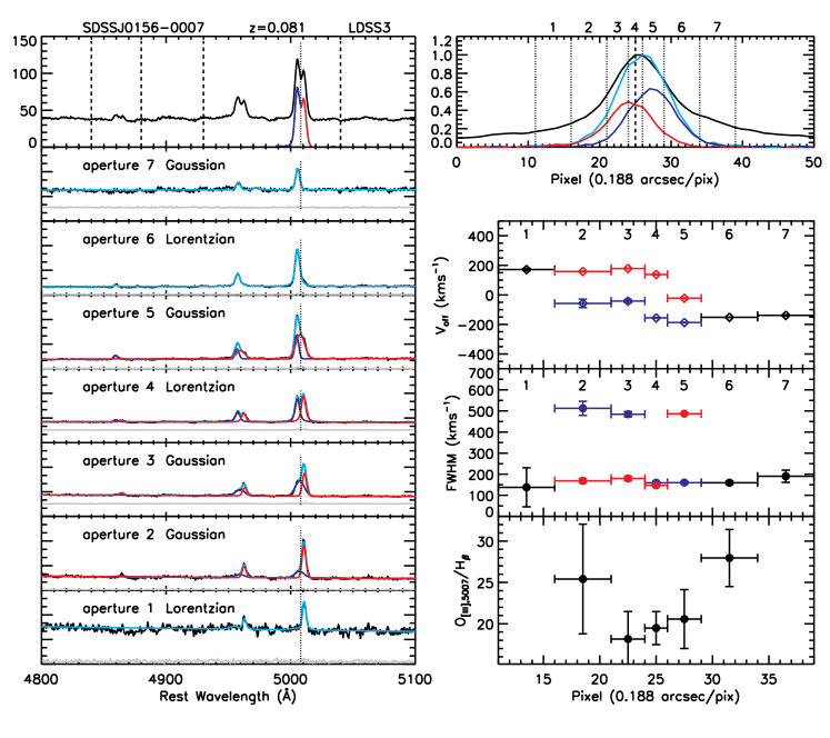
Figure 18: Diagnosis of the 2d spectrum of J0156$-$0007. Notation is the same as Fig. 3. Deblending of the two velocity components is ambiguous in several spatial bins. The [O III]/H$\beta$ flux ratio varies within $\sim 0.2$ dex in bins for which we have measurements. Weak velocity gradients can been seen for both [O III] components.

J0156$-$0007. Fig. 17 shows the $K_{s}$ image and the 2d spectrum for this object. A disk morphology is apparent in the NIR image. The two velocity components of [O III] are spatially offset by $\sim 0.7$″, with no corresponding pair of nuclei seen in the NIR. Fig. 18 shows the 1d slices of the 2d spectrum at different distances from the peak of the continuum emission. The [O III] $\lambda$5007/H$\beta$ flux ratio is almost constant at each aperture location. Weak velocity gradients can been seen for both [O III] components. At most locations the line width is narrow, which suggests that coherent rotation is the dominant motion. This object is best explained by a rotational [O III] disk, with an asymptotic flat rotation velocity $V_{c}\sin i\sim 150\,{\rm kms^{-1}}$.

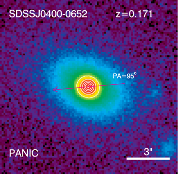
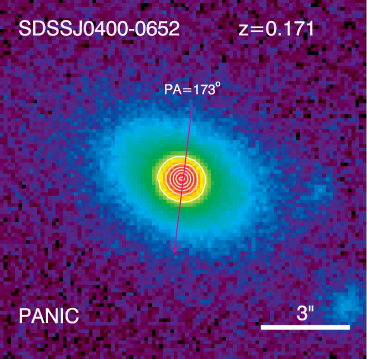
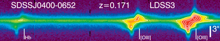
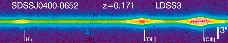
Figure 19: SDSS J0400$-$0652 (NLR kinematics). Upper: PANIC NIR image in $K_{s}$. This object has no resolved double nucleus. Two slit positions are shown. Bottom: LDSS3 2d spectrum for the H$\beta$-[O III] region with corresponding lines marked (note that the locations of these line marks are approximate). The 2d spectrum shows a rich kinematic structure at one slit position, but not at the other slit position. Notation is the same as Fig. 2.

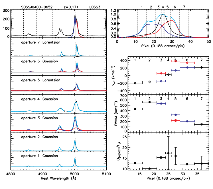
Figure 20: Diagnosis of the 2d spectra of J0400$-$0652. Notation is the same as Fig. 3. The upper panel is for the slit position PA$=95^{\circ}$ and the bottom panel is for the slit position PA$=173^{\circ}$. The two slit positions show very different distributions of the line emission. Deblending of the two velocity components is ambiguous in most spatial bins because of the complicated kinematics as seen in the 2d spectrum.

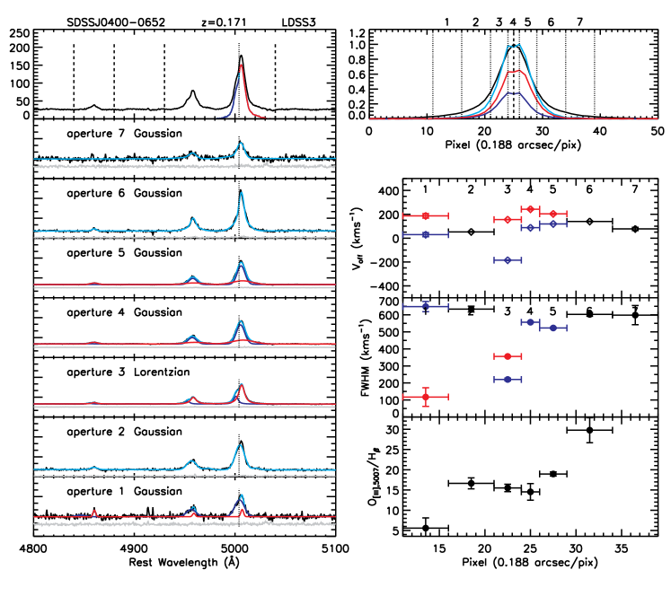
Figure 20: Continued.

J0400$-$0652. This object shows a smooth single profile in the $K_{s}$ image, while its slit spectra show spatially resolved [O III] emission extending to $\sim 3$″. A subsequent NIR AO image obtained by Fu et al. (2010) did not reveal a double nucleus at $\sim 0.1$″ resolution. In Fig. 19 we show its $K_{s}$ image and 2d spectra at two position angles, and in Fig. 20 we show the 1d spectral diagnostics. The 2d spectrum along PA$=95^{\circ}$ shows rather complicated [O III] emission region kinematics. It shows a high velocity dispersion near the center, and some velocity gradient along the slit direction, which is indicative of disk rotation and/or outflows. Clearly there are more than two [O III] components. On the other hand, the 2d spectrum along PA$=173^{\circ}$ shows much less structure, which is presumably caused by the different spatial coverage. This object is best explained by NLR kinematics, possibly involving both outflows and rotation. A more detailed follow-up of this object (i.e., with IFU or multiple-slit spectroscopy) is highly desirable to resolve the [O III] kinematics map.

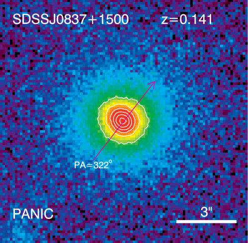
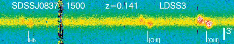
Figure 21: SDSS J0837+1500 (NLR kinematics). Upper: PANIC NIR image in $K_{s}$. This object has no resolved double nucleus. Bottom: LDSS3 2d spectrum for the H$\beta$-[O III] region with corresponding lines marked (note that the locations of these line marks are approximate). The two velocity components are spatially offset by $\sim 1.3$″. Notation is the same as Fig. 2.

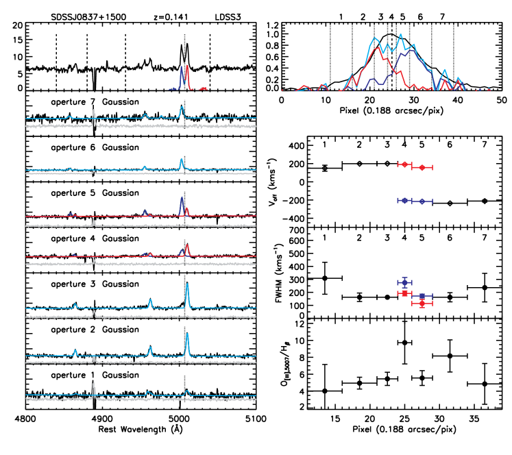
Figure 22: Diagnosis of the 2d spectrum of J0837+1500. Notation is the same as Fig. 3. The two [O III] components are comparable in line strength and symmetric about the center of the continuum. No obvious trends are seen in the velocity offset and line width of the two [O III] components. There is some indication that the [O III]/H$\beta$ flux ratio increases towards the center of the continuum emission, which may suggest that the ionizing source is coincident with the center of the continuum.

J0837+1500. Fig. 21 shows the $K_{s}$ image and the 2d spectrum for this object. The two velocity components of [O III] are spatially offset by $\sim 1.5$″, with no corresponding pair of nuclei seen in the NIR. Fig. 22 shows the 1d slices of the 2d spectrum at different distances from the peak of the continuum emission.

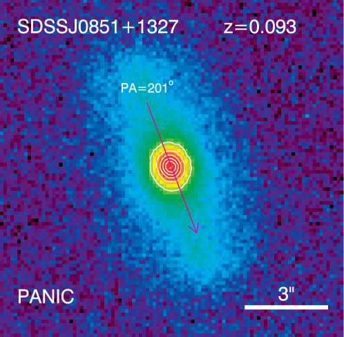
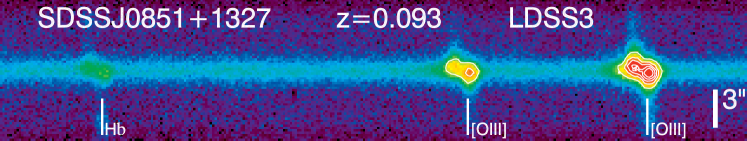
Figure 23: SDSS J0851+1327 (NLR kinematics). Upper: PANIC NIR image in $K_{s}$. This object has no resolved double nucleus. Bottom: LDSS3 2d spectrum for the H$\beta$-[O III] region with corresponding lines marked (note that the locations of these line marks are approximate). The two velocity components are spatially offset by $\sim 0.6$″. Notation is the same as Fig. 2.

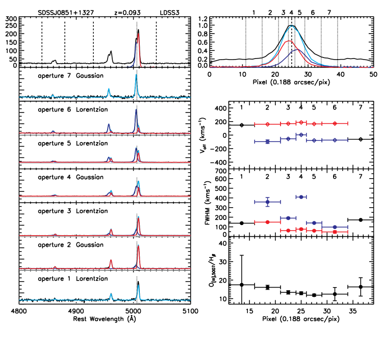
Figure 24: Diagnosis of the 2d spectrum of J0851+1327. Notation is the same as Fig. 3. This object has a giant disk component seen in the optical image and 2d spectrum, which is also seen in the extended distribution of the continuum emission in the upper-right panel. No obvious trends are seen for the velocity offset and line with of the two [O III] components. The [O III]/H$\beta$ flux is constant within $\sim 0.1$ dex.

J0851+1327. Fig. 23 shows the $K_{s}$ image and the 2d spectrum for this object. The two velocity components of [O III] are spatially offset by $\sim 0.6$″, with no corresponding pair of nuclei seen in the NIR. This galaxy has an edge-on disk component seen in the NIR, which is also seen in its SDSS optical image and the 2d spectrum shown in Fig. 24. This object is best explained as a rotational [O III] disk, given the disk morphology seen in the NIR and in the optical.

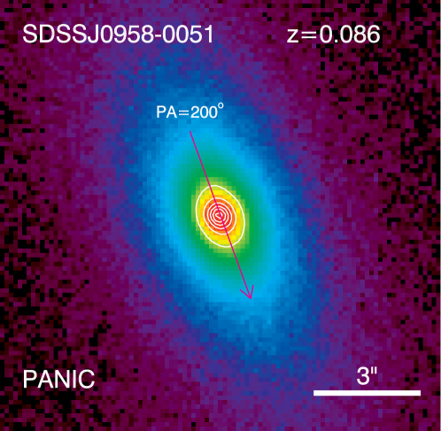
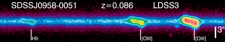
Figure 25: SDSS J0958$-$0051 (NLR kinematics). Upper: PANIC NIR image in $K_{s}$. This object has no resolved double nucleus, and it has a large disk component. Bottom: LDSS3 2d spectrum for the H$\beta$-[O III] region with corresponding lines marked (note that the locations of these line marks are approximate). The two velocity components are spatially offset by $\sim 0.8$″. There are clear velocity gradients in the line emission. Notation is the same as Fig. 2.

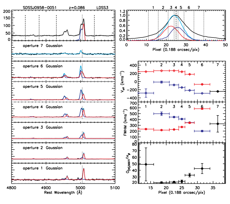
Figure 26: Diagnosis of the 2d spectrum. Notation is the same as Fig. 3. Velocity gradients can been seen for both the blueshifted and redshifted components, which is indicative of rotation. The FWHM of the two velocity components show peculiar patterns, which do not seem to be caused by failed deblending, and is suggestive of more complicated kinematics in this system. The [O III]/H$\beta$ flux ratio seems to rise towards the outermost bins, which may by caused by density stratification.

J0958$-$0051. Fig. 25 shows the $K_{s}$ image and the 2d spectrum for this object. A disk component is seen in the NIR image. The two velocity components of [O III] are spatially offset by $\sim 0.8$″, with no corresponding pair of nuclei seen in the NIR. Fig. 26 shows the 1d slices of the 2d spectrum at different distances from the peak of the continuum emission. Velocity gradients are clearly seen for both [O III] components. This object is best explained by a rotational [O III] disk.

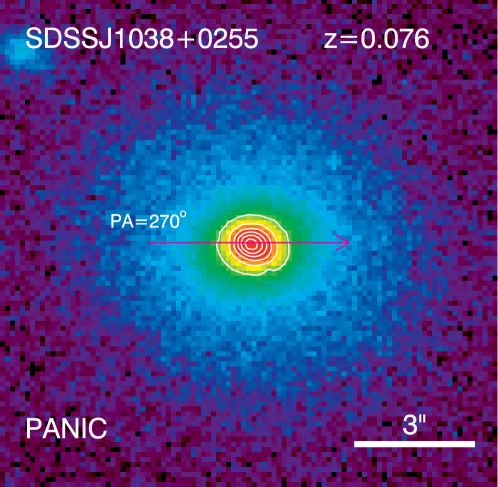
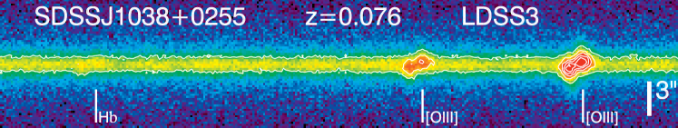
Figure 27: SDSS J1038+0255 (NLR kinematics). Upper: PANIC NIR image in $K_{s}$. This object has no resolved double nucleus. Bottom: LDSS3 2d spectrum for the H$\beta$-[O III] region with corresponding lines marked (note that the locations of these line marks are approximate). The two velocity components are spatially offset by $\sim 0.9$″. Notation is the same as Fig. 2.

J1038+0255. Fig. 27 shows the $K_{s}$ image and the 2d spectrum for this object. The two velocity components of [O III] are spatially offset by $\sim 1$″, with no corresponding pair of nuclei seen in the NIR. This object is best explained by either a rotational [O III] disk or biconical outflows.

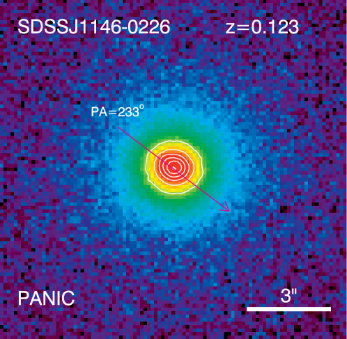
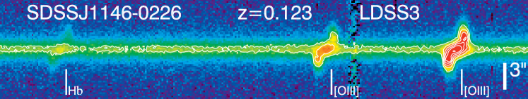
Figure 29: SDSS J1146$-$0226 (NLR kinematics). Upper: PANIC NIR image in $K_{s}$. This object has no resolved double nucleus. Bottom: LDSS3 2d spectrum for the H$\beta$-[O III] region with corresponding lines marked (note that the locations of these line marks are approximate). This object shows a clear rotation curve. The two velocity components are spatially offset by $\sim 1.3$″ measured from the centroids of the blue- and red-shifted emission. Notation is the same as Fig. 2.

J1146$-$0226. Fig. 29 shows the $K_{s}$ image and the 2d spectrum for this object. The $K_{s}$ image shows a smooth single stellar bulge, while the 2d spectrum shows a clear rotation-curve like velocity gradient across the slit. Under poor spatial resolution or if the object were observed at higher redshifts, the rotation-curve would be unresolvable, and the [O III] emission would appear as two distinct velocity components spatially offset by $\sim$ a few kpc. This object is best explained by a rotational [O III] disk.

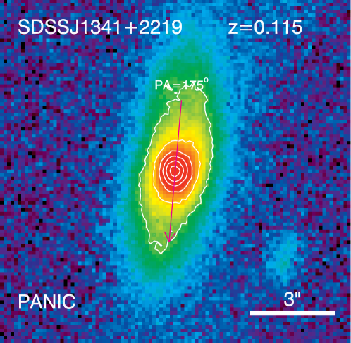
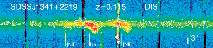
Figure 31: SDSS J1341+2219 (NLR kinematics). Upper: PANIC NIR image in $K_{s}$. This object has no resolved double nucleus, although it has a disturbed disk component. Bottom: DIS 2d spectrum for the H$\alpha$ region with corresponding lines marked (note that the locations of these line marks are approximate). The DIS spectrum for the H$\beta$-[O III] region has poor quality. The two velocity components are spatially offset by $\sim 1.7$″ measured from the peaks of the blueshifted and redshifted H$\alpha$ emission. Notation is the same as Fig. 2.

J1341+2219. Fig. 31 shows the $K_{s}$ image and the 2d spectrum for this object. A disk component is seen in the NIR image. The [O III]-H$\beta$ part of our 2d spectrum has low quality so we show the H$\alpha$ region instead. The two NEL velocity components are spatially offset by $\sim 1.7$″, with no corresponding pair of nuclei seen in the NIR. This object is best explained by a rotational [O III] disk.

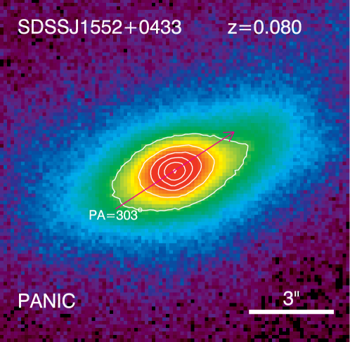
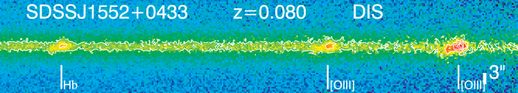
Figure 32: SDSS J1552+0433 (NLR kinematics). Upper: PANIC NIR image in $K_{s}$. This object has no resolved double nucleus, although it has a disturbed disk component in the optical and in the NIR. Bottom: DIS 2d spectrum for the H$\beta$-[O III] region with corresponding lines marked (note that the locations of these line marks are approximate). The two velocity components are spatially offset by $\sim 1.2$″. Notation is the same as Fig. 2.

J1552+0433. For this object the two [O III] components are spatially offset by $\sim 1.2$″ in their peak emission, as seen from its 2d spectrum shown in Fig. 32. Its $K_{s}$ image shows a disk component, which seems to be warped at the north-west edge. Nevertheless, two stellar bulge components separated by $\sim 1.2$″ would have been seen in the NIR image if this object were a kpc-scale binary AGN. Thus we classify this object in the NLR kinematics category.

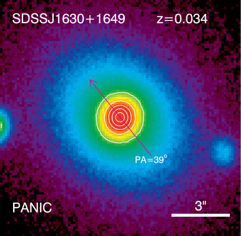
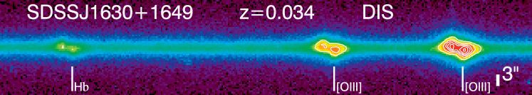
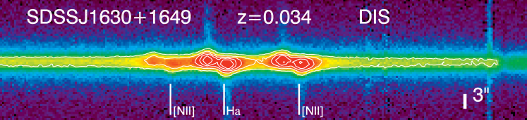
Figure 33: SDSS J1630+1649 (NLR kinematics). Upper: PANIC NIR image in $K_{s}$. This object has no resolved double nucleus, and it has a faint companion $\sim 5$″ away towards the east. Middle and Bottom: DIS 2d spectrum for the H$\beta$-[O III] and H$\alpha$ regions with corresponding lines marked (note that the locations of these line marks are approximate). The two [O III] components are spatially offset by $\sim 0.8$″. Notation is the same as Fig. 2.

J1630+1649. Fig. 33 shows the $K_{s}$ image and the 2d spectrum for this object. The two [O III] velocity components are spatially offset by $\sim 0.8$″, with no corresponding pair of nuclei seen in the NIR. A recent NIR AO image of this object at $\sim 0.1$″ resolution did not show a double nucleus either (Fu et al., 2010). This object is best explained by a rotational [O III] disk.

J2304$-$0933. For this object the NIR image shows a clear disk component. The seeing was quite poor for the slit spectroscopy observation, but the two NEL components seem to be spatially offset by $\sim 0.8$″ in their peak emission. A recent NIR AO image of this object reveals no double nucleus at $\sim 0.1$″ resolution (Fu et al., 2010). It is thus most likely a case of NLR kinematics.

While many of these NLR kinematics cases show a clear disk morphology in imaging data, a few objects, such as J0837+1500 and J1146-0226, show an early-type morphology. The ionized gas emission in these early-type hosts is extended on kpc scales. Emission line kinematics studies of local early-type galaxies often show ionized gas emission to kpc scales, and the gas kinematics is usually decoupled from the stellar kinematics (e.g., Sarzi et al., 2006), which is consistent with our findings here. However, the emission line strength is much stronger in our AGNs, which may indicate a larger gas reservoir in these early-type hosts than their local counterparts.

3.3 Ambiguous Cases

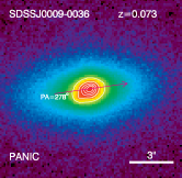
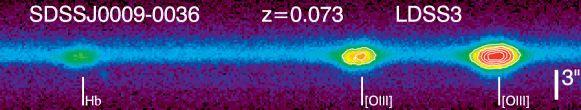
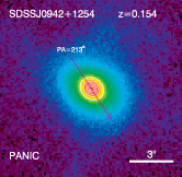
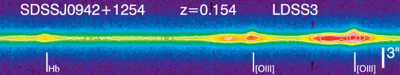
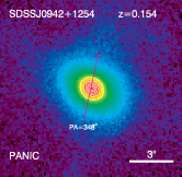
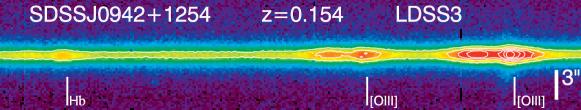
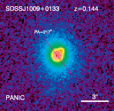
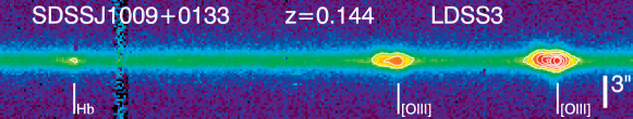
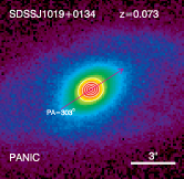
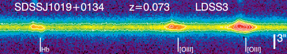
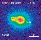
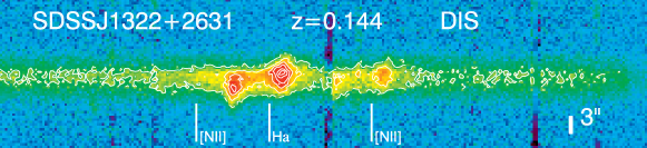
Figure 36: PANIC NIR images and 2d spectra for objects classified as ambiguous cases. In all objects except for SDSS J1322+2631, the spatial offset between the two emission line velocity components is smaller than the typical resolution of our NIR imaging.

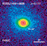
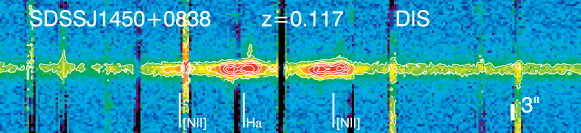
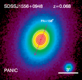
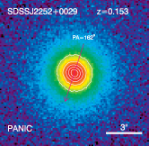
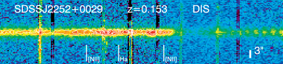
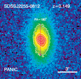
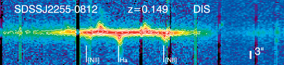
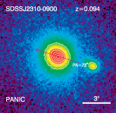
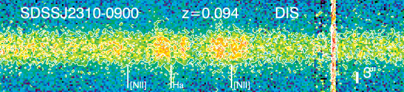
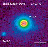
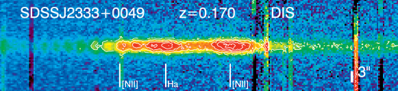
Figure 36: Continued.

About $40\%$ of objects that appear single in NIR imaging were classified as ambiguous cases, i.e., the combined NIR imaging and slit spectroscopic data are insufficient to distinguish between the binary scenario and the kinematics scenario. In essentially all of these cases, the two velocity components of the [O III] emission have undetectable or small spatial offset that is below the resolution limit of the NIR imaging (i.e., $\lesssim 0.4$″). In the binary scenario, the two BHs and their associated stellar components would have smaller projected separations, which would need higher-resolution observations such as ground AO imaging (e.g., Fu et al., 2010) or space-based observations to resolve the pair of nuclei. Nevertheless the real separation between the two BHs is unlikely to be much less than $\sim$ kpc because NLRs have intrinsic sizes of hundreds of pc or above. In the case of NLR kinematics (rotation or outflows), either the relevant scale is below one or two kpc, or the slit position happens to be perpendicular to the outflow axis or the rotational disk (cf., see Fig. 19 for J0400$-$0652). Fig. 36 shows the NIR images and 2d spectra for these objects. We now briefly comment on individual objects in this category.

J0009$-$0036. In this object the two [O III] components are spatially offset by $<0.2$″ in the 2d spectrum, and the NIR image shows a single nucleus. Its NIR image shows a minor structure $\sim 1$″ south-east from the center of the peak NIR emission, which is not contributing to the [O III] emission. A better slit position and higher resolution imaging and spectroscopy are needed to rule out the existence of a companion at $<0.2$″ separation.

J0942+1254. This object was observed with two slit positions. Both of the 2d spectra show no spatial offset ($<0.2$″) between the two [O III] velocity components. No double nucleus was seen in the NIR image. However, the optical and NIR images of this object show spectacular tidal features, indicative of recent mergers. This object deserves a higher-resolution observation, and we suspect it is likely to be a small projected separation binary AGN.

J1009+0133. This object shows a minor companion $\sim 1$″ north-west of the peak emission in the NIR image. Unfortunately due to our slit position, we couldn’t confirm that these two stellar nuclei correspond to the two [O III] components seen in the 2d spectrum. Although the NIR image alone is suggestive of a binary, a new slit position is needed to test this hypothesis.

J1019+0134. The NIR image shows a disturbed morphology in the outskirts, indicative of a recent merger event. The two [O III] components are spatially offset by $\sim 0.3$″ as shown in the 2d spectrum. Seeing in the NIR is $\sim 0.7$″. This could either be a binary or NLR kinematics. New slit spectroscopy with a different position angle and/or better spatial resolution are needed to distinguish the two scenarios.

J1322+2631. For this object we only have a slit spectrum covering the H$\alpha$ region. The two narrow line components are spatially offset by $\sim 2.1$″ as shown in the 2d spectrum. In the $K_{s}$-band image we see two main stellar nuclei separated by $\sim 2.3$″, and there is also a third (minor) companion to the southwest, about $2.5$″ from the central brightest stellar component. A close examination of the 2d spectrum suggests that the two [O III] components are probably not spatially coincident with the two main stellar nuclei, even though their separation happens to be consistent with that of the two stellar nuclei. If this were true, it would imply a kinematic origin for the double-peaked [O III] emission in this object. However, the seeing in our 2d optical spectrum is poor and the locations of the stellar continua are not well determined. Hence it is still possible that the two spatially offset [O III] components are coincident with two of the three stellar components seen in the NIR image. The poor seeing in the spectrum also prohibited measurements of the absorption redshifts of the northeast and southwest companions, whose continua are blended with the continuum of the brighter central source. A new slit spectrum with better spatial resolution is needed to draw firm conclusions on this object.

J1450+0838. The 2d spectra shows that the two [O III] components are consistent with no spatial offset ($<0.2$″). The NIR image shows a single nucleus at $\sim 0.8$″ resolution.

J1556+0948. The two [O III] components are offset by $\sim 0.4$″ in the 2d spectrum, and the NIR image shows a single nucleus at $\sim 0.6$″ resolution. The double-peaked emission lines in this source are likely to be due to NLR kinematics, but higher-resolution NIR imaging data is needed to rule out the binary scenario.

J2252+0029. The two NEL components are consistent with no spatial offset in the 2d spectrum. Higher-resolution imaging observation and/or different slit positions are required to distinguish the binary and the NLR kinematics scenarios.

J2255$-$0812. The NIR image shows a disturbed disk component, and the two NEL components show a small spatial offset, $\lesssim 0.5$″, in the 2d spectrum. Extended line emission is seen on opposite sides of the central continuum, which is caused by ionized gas in the rotating galactic disk. This object is likely a case of NLR kinematics, but a higher resolution imaging observation and/or different slit positions are needed to rule out the binary scenario.

J2310$-$0900. This object has a companion $\sim 4$″ away, which does not contribute to the [O III] emission seen in the SDSS fiber spectrum. The companion is too faint to measure its redshift in our slit spectrum. The seeing was quite poor for the slit spectroscopy observation, and the two NEL components are consistent with no spatial offset. A better quality slit spectrum and/or different slit positions are needed to distinguish the binary and the NLR kinematics scenarios.

J2333+0049. This object has a minor companion about $6$″ to the southeast, which is too faint to measure its redshift in our slit spectrum. The two NEL components are consistent with no spatial offset in the 2d spectrum. It appears single in our NIR imaging and in the recent NIR AO imaging (Fu et al., 2010) at $\sim 0.1$″ resolution.

4 Discussion

4.1 The Bulk Properties of Kpc-scale Binary Type 2 AGNs

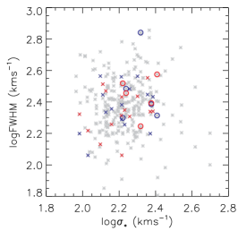
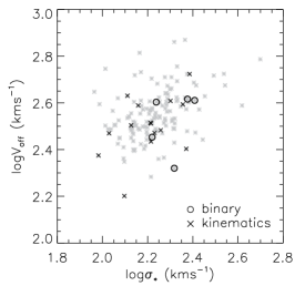
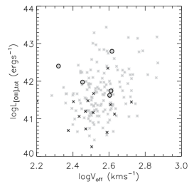
Figure 37: Bulk properties of the five objects classified as binary AGNs (circles) compared with those classified as NLR kinematics in single AGNs (crosses). In all panels, the gray points are for all objects in the double-peaked sample of Liu et al. (2010b). Left: Distributions in the plane of FWHM and stellar velocity dispersion $\sigma_{*}$. The stellar velocity dispersions are for the whole galaxy within the 3″ diameter fiber and the FWHMs are for the two velocity components (the blueshifted component is indicated in blue and the redshifted component is indicated in red). Measurements are taken from Liu et al. (2010b). Middle: Distributions in the plane of $\sigma_{*}$ versus velocity offset between the two components, $V_{\rm off}$. Right: Distributions in the plane of the total [O III] $\lambda$5007 luminosity vs $V_{\rm off}$.

Bearing in mind the small-number statistics of our sample, in Fig. 37 we compare the bulk properties of kpc-scale binary AGNs (circles) and those that originate from NLR kinematics (crosses), measured from spatially-integrated SDSS fiber spectra (Paper I). The left panel shows the FWHM of each [O III] component as a function of the fiber-integrated stellar velocity dispersion. The red and blue symbols are for the redshifted component and the blueshifted component, respectively; the gray symbols are for all the objects in our parent sample (Paper I). The five binary AGNs all reside in the right half of the plot, with larger stellar velocity dispersions on average. This is consistent with the existence of multiple stellar systems in these binary AGNs. The middle panel shows the velocity offset of the two [O III] components as a function of the stellar velocity dispersion. The right panel shows the total [O III] $\lambda$5007 luminosity versus the [O III] velocity offset. The binary AGNs seem to occupy a different luminosity regime from those classified as NLR kinematics. Fig. 37 suggests that the bulk properties of kpc-binary AGNs might be statistically different from those with an origin in NLR kinematics, which, if true, can be used to refine the selection of binary candidates from spatially-integrated spectroscopy. However, our current sample of kpc-scale binary AGNs is still small, and a larger statistical sample of binary AGNs is needed to confirm these trends.

In these binary systems, the smaller stellar component does not necessarily correspond to the more luminous [O III] component. If BH mass is proportional to bulge mass/luminosity and [O III] luminosity is proportional to the intrinsic AGN luminosity, then the smaller BH must be accreting at a substantially higher Eddington ratio than the larger BH in J1131$-$0204 and J1332+0606. It is likely that the smaller component in these merging systems is more gas-rich and/or easier for the nuclear region to be disturbed during the merger, and hence the BH accretion is more efficient.

4.2 The Frequency of Kpc-scale Binary Type 2 AGNs

Although we have only followed up a small fraction of the double peaked [O III] type 2 AGNs in our sample (Paper I), the $\sim 30$ objects with both NIR imaging and slit spectroscopic data presented in this paper allow us to estimate the fraction of kpc-scale AGNs among these double-peaked [O III] AGNs. For most of our targets we carried out the imaging first, and promising targets seen in the imaging data were preferentially observed spectroscopically. We have obtained slit spectra for only about half of the imaged objects. Therefore we must estimate the fraction of binary AGNs and NLR kinematics taking into account the spectroscopic completeness. Of the $61$ objects that we have observed in the NIR, five were classified as kpc-scale binary AGNs with resolved double nuclei that are within the $3$″ diameter of SDSS fibers, and subsequently confirmed with slit spectroscopy. Hence the frequency of kpc-scale binary AGNs among these double-peaked [O III] objects is $\sim 10\%$. Of the remaining $\sim 90\%$ of the objects, $\sim 50\%$ are best explained by NLR kinematics (§3.2) and $\sim 40\%$ are ambiguous cases. At least some of the latter case are of NLR kinematics origin, and the remainder are probably binary AGNs with somewhat smaller separations, and could be identified with better spatial resolution observations (e.g., Fu et al., 2010). If we take the results of Fu et al. (2010) and assume all the objects with resolved double nuclei in their NIR AO imaging are binary AGNs (but see §4.3), then the binary AGN fraction among the double-peaked [O III] objects increases to $\sim 20\%$. It is conceivable (although unlikely) that kpc-scale binary AGNs with even smaller separations would not have been revealed with NIR AO imaging, and if we assume this entire ambiguous sample is binaries, we get a hard upper limit of the kpc-scale binary AGN fraction of $\sim 50\%$. Therefore, a conservative estimate of the genuine kpc-binary AGN fraction of the double-peaked [O III] type 2 AGNs is $10\%\lesssim f_{1}<50\%$ and the upper bound should be considered as a hard limit. Our observations thus indicate that the majority of these double-peaked [O III] objects reflect NLR kinematics and are not kpc-scale binary AGNs. However, in some of the systems that we classified as kinematic cases, we see disturbed morphology or close companions, which may indicate that the (single) AGN activity was triggered by a recent merger event.

Only $\sim 1\%$ of low-redshift ($z<0.3$) type 2 AGNs have double-peaked [O III] profiles in their spatially-integrated spectra (Paper I). If the orbit inclination is random for binary AGNs, then some of them will not show a double-peaked [O III] profile since the line itself has a finite width (due to the intrinsic line width and instrument broadening), and thus will not enter our sample. The real situation is more complicated. The selection completeness depends on the spectral resolution of SDSS, and the intrinsic distributions of binary properties, such as the relative velocity of the two BHs at $\sim$ kpc separations, and the FWHM and strength of individual narrow line components. The SDSS spectral resolution will exclude double-peaked [O III] objects with a relative velocity offset $\lesssim 150\,{\rm kms^{-1}}$, and our sample in Paper I is strongly biased against weak [O III] objects. In Paper I we performed simple Monte Carlo simulations of mock spectra to estimate the selection completeness of kpc binaries with double-peaked [O III] with assumed distributions of kpc-scale binary AGN properties, combined with the SDSS spectral resolution and random line-of-sight (LOS). We found that the selection completeness rapidly decreases with decreasing the LOS velocity offset, decreasing the [O III] equivalent width, and increasing the line FWHM; and all these effects are well coupled.

Here we perform similar Monte Carlo simulations, with reasonable properties that are appropriate for our sample. We assume a physical relative velocity offset of $500\,{\rm km\,s^{-1}}$ between the two velocity components (i.e., both NLRs are on circular orbits with circular velocities of $250\,{\rm km\,s^{-1}}$), a fixed FWHM$=250\,{\rm km\,s^{-1}}$ for both components, and assign an [O III] $\lambda$5007 rest equivalent width EW${}_{\rm[OIII]5007}\equiv 3$EW_[OIII]4959 uniformly distributed within $15-45\,$Å for each component. The assumed circular velocity of the binary is reasonable given that our objects are massive galaxies with stellar mass $M_{*}\sim 10^{11}\,M_{\odot}$, and the adopted FWHM and EW values are also typical of our sample objects (Paper I). We further assume random orientations of the binary orbits, and generate mock spectra with the assumed [O III] properties, a continuum S/N$\sim 5$ pixel^-1, and the SDSS spectral resolution. We visually inspect these mock spectra and flag double-peaked objects. We found $\sim 20\%$ of the simulated objects are identified as double-peaked [O III] objects. As discussed earlier, 10-50% of double-peaked objects have compelling evidence for two active nuclei ($f_{1}$). Now assuming that we can detect only $20\%$ of true double-peaked objects, we expect that $5\%$ of the $z\lesssim 0.3$ type 2 AGN population is double, and thus that a fraction $0.5\%<f_{2}=5\%\times f_{1}<2.5\%$ of the total population is composed of kpc-scale binaries. It is very likely that there are populations of kpc-scale binary AGNs with a relative (unreduced) orbital velocity $\lesssim 150\,{\rm kms^{-1}}$ or with more discrepant [O III] luminosity ratios that are missed in our SDSS sample.

At face value, this low fraction of kpc-scale binary AGNs is at odds with the hypothesis that AGNs are triggered by major mergers. It either implies that the fraction of time that a binary AGN spends during this kpc phase is very small compared to the total AGN lifetime, or only a tiny fraction of kpc-scale binary AGNs have two distinct NLRs with comparable luminosity and are lit up simultaneously. Alternatively, it could be that major mergers are not the dominant mechanism for triggering low-luminosity AGN activity at low redshift, since the fueling rate is not as stringent for AGNs as for luminous quasars, and alternative fueling routes (i.e., secular processes and minor mergers) may suffice. Refining the binary AGN fraction at various separations and combining with numerical simulation results are needed to sort out these possibilities, and our current study represents the first step towards quantifying the demographics of binary AGNs on kpc scales.

4.3 The Different Behaviors of Gas and Stars

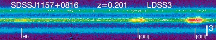
Figure 38: A slit spectrum for J1157+0816, which shows three nuclei in the optical SDSS image (Smith et al., 2010) and in the NIR image (Fu et al., 2010). The slit was placed across the three nuclei. Only the central nucleus has [O III] emission, which is responsible for the double-peaked [O III] profile seen in the SDSS spectrum.

Our NIR imaging and optical slit spectroscopy demonstrate the importance of combining imaging and spectroscopy data in confirming the binary AGN nature of double-peaked objects. Objects that show spatially offset [O III] emission in slit spectra are not necessarily kpc-scale binary AGNs, as seen in most of the cases ascribed to NLR kinematics discussed in §3.2. Likewise, objects that show apparent double nuclei in the NIR imaging are not necessarily kpc-scale binary AGNs, as the companion may not have [O III] emission at all. Objects such as J0002$+$0045 presented in this paper clearly demonstrate the latter case. For the same reason, not all of the objects with resolved multiple nuclei in Fu et al. (2010) are binary AGNs, even if these multiple nuclei are covered in a single SDSS fiber. For example, J1157$+$0816 shows three components in both optical and NIR imaging (Smith et al., 2010; Fu et al., 2010). However, neither the upper or lower companions in the slit spectrum (Fig. 38) show [O III] emission (although both are at the redshift of the central object), and the double-peaked [O III] emission is likely caused by the NLR kinematics of the central source.

5 Conclusions

We have presented NIR imaging and optical slit spectroscopic data for 31 double-peaked [O III] type 2 AGNs drawn from the sample of Paper I. The combination of imaging and spectroscopy allows us to identify the origin of the double-peaked [O III] emission in these peculiar objects. Our main conclusions are:

• $\sim 10\%$ of these objects show spatially coincident double stellar nuclei and NLR emission. The two spatially offset [O III] emission components are also separated in velocity, and lead to the double-peaked profile seen in the spatially-integrated spectra. These objects are best explained by a pair of merging AGNs separated on kpc scales.

• $\sim 50\%$ of these objects show a single smooth stellar component at $\sim 0.6$″ resolution, while the two [O III] velocity components are spatially offset by $\gtrsim 0.6$″. For objects with sufficient spectral quality we usually see velocity (or velocity dispersion) gradients indicative of a kinematic signature. These objects are best explained by NLR kinematics in single AGNs, involving rotation and/or outflows. A recent study of a single double-peaked [O III] AGN (SDSS J1517+3353) also favors the kinematics explanation (Rosario et al., 2010).

• The remaining $\sim 40\%$ of these objects show a small ($\lesssim 0.4$″) spatial offset between the two [O III] velocity components and a single smooth stellar component. Some of these objects are likely binaries at smaller separations (e.g., Fu et al., 2010), with the remainder likely due to NLR kinematics at smaller scales. Follow-up observation with better spatial resolution is needed to distinguish between the two scenarios.

• Our observations demonstrate the necessity of combining imaging and slit spectroscopy data to identify bona fide kpc-scale binary AGNs. In particular, objects that show spatially offset [O III] components are not necessarily binary AGNs, nor are those objects that show spatially resolved stellar components.

• We estimate that $\sim 0.5-2.5\%$ of the local ($z<0.3$) type 2 AGNs are kpc-scale binary AGNs in a major merger, where both components are obscured type 2 AGN with comparable [O III] luminosities.

Our follow-up observations of the double-peaked [O III] sample demonstrate the feasibility of selecting kpc-scale binary AGN candidates using this particular spectroscopic feature, with a $\gtrsim 10\%$ success rate. So far we have only followed up about one third of our parent sample and already doubled the number of known kpc-scale binary AGNs. Our imaging and spectroscopy follow-up is still ongoing, accompanied by detailed investigations on individual systems in other wavelengths and/or with better spatial resolution. A natural step forward would be AO imaging and IFU spectroscopy of merging systems and systems with outflows to obtain detailed spatial and kinematic maps. By the end of our survey, we expect to increase the number of known kpc-scale binary AGNs by an order of magnitude. The increased statistics of the kpc-scale binary AGN sample will improve the estimate of the binary fraction and the study of bulk properties of kpc-scale binary AGNs, and will shed light on the effects of mergers on the host and AGN activity in these systems. In the meantime, there is strong need to explore the parameter space in merger simulations to confront the observed statistics (e.g., Blecha et al. 2010, in preparation).

Appendix A Model Fits for the NIR Images of Kinematic and Ambiguous Cases

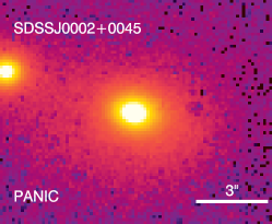
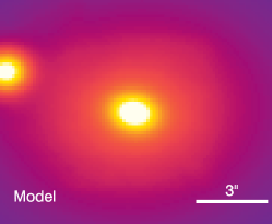
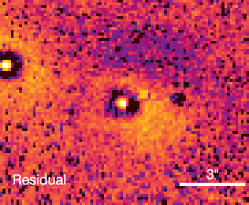
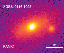
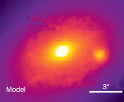
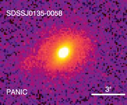
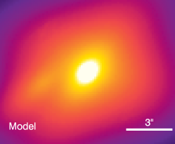
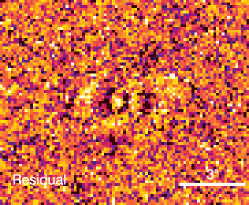
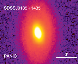
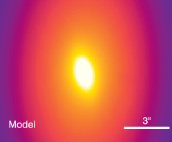
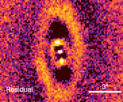
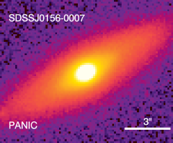
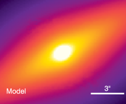
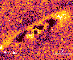
Figure 39: Model fits of the NIR surface brightness for objects classified as NLR kinematics of single AGNs (§3.2) using GALFIT. The first column shows the data, the second column shows the models and the last column shows the residuals. Note that the residual maps have been re-stretched to enhance the contrast and the residuals are not important compared to the observed fluxes (the apparent excess seen in some of the residual maps has values less than $5\%$ of the observed fluxes at the corresponding locations).

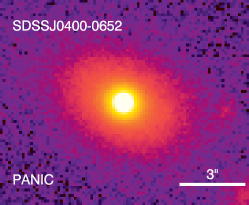
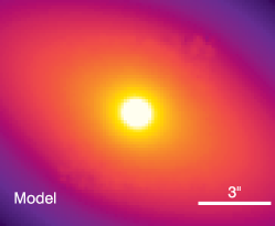
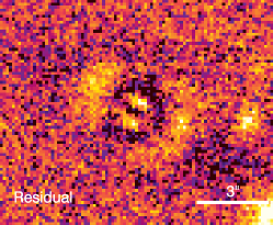
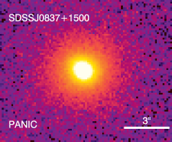
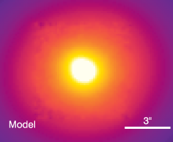
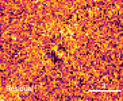
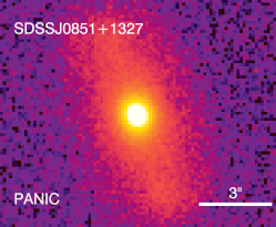
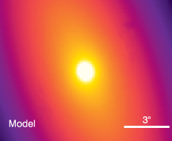
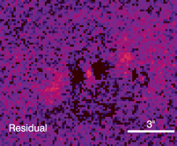
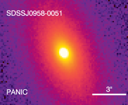
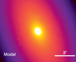
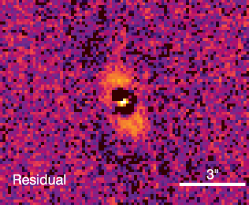
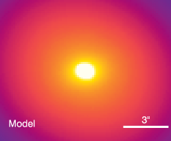
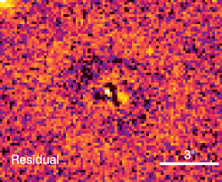
Figure 39: Continued.

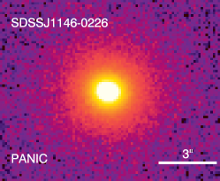
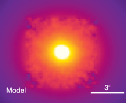
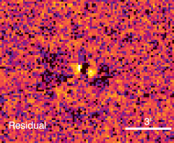
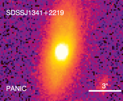
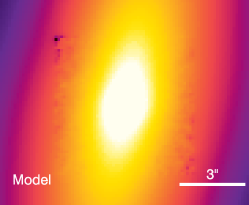
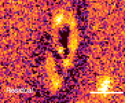
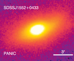
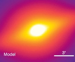
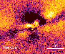
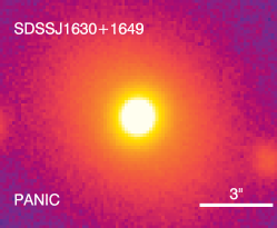
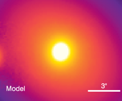
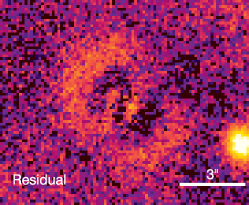
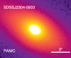
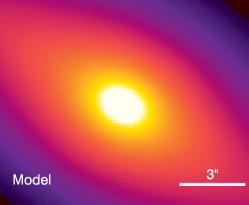
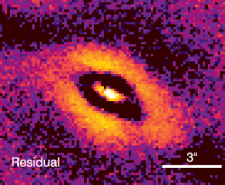
Figure 39: Continued.

For completeness we here provide the GALFIT results for objects that we classified as NLR kinematics around single AGNs or ambiguous cases. Even though these AGNs do not appear to have substantial multiple components within the host galaxy, reproducing the exact surface brightness profile is still challenging for some cases. We restrict ourselves to a basic model of a de Vaucouleurs bulge $+$ an exponential disk for the whole galaxy. We also tried a Sérsic bulge plus an exponential disk to improve the fits if possible. In a few objects there are one or two companions overlapping with the light from the galaxy, and we fit additional components to these companions. The fitting results are shown in Figs. 39 (for the NLR kinematics cases) and 40 (for the ambiguous cases). In the NLR kinematics cases, no substantial residuals are seen at the locations indicated by the offset [O III] emission seen in the 2d spectra.

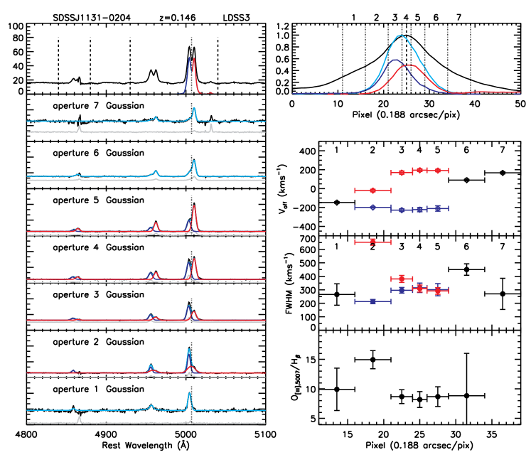
Figure 5: Diagnosis of the 2d spectrum of J1131-0204. Notation is the same as Fig. 3. The spatial distribution of the continuum shown in the upper-right panel has extended wings, which arise from the prominent disk as seen in the optical and NIR images. There are no coherent trends seen in the velocity offsets, line widths and [O III]/H$\beta$ flux ratio, as functions of location.

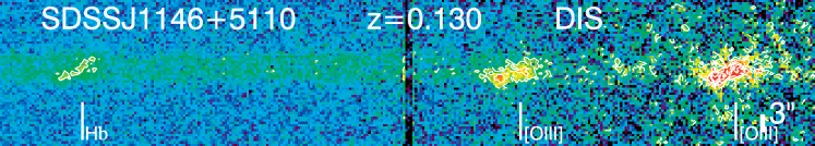
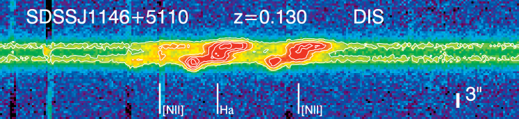
Figure 6: SDSS J1146+5110 (binary). Upper: DIS 2d spectrum for the H$\beta$-[O III] region. Bottom: DIS 2d spectrum for the H$\alpha$ region with corresponding lines marked (note that the locations of these line marks are approximate). We do not have a PANIC image for this object, but its 2MASS image shows two nuclei separated by $\sim 2.7$″. The two continua of this system are apparent in the bottom spectrum due to the relatively large separation of the two nuclei. The line emission in the southern nucleus itself has two velocity components. The line emission in the northern nucleus is spatially offset by $\sim 2.5$″ from the continuum of the southern nucleus, and is very weak in the H$\beta$-[O III] region due to poor spectral quality.

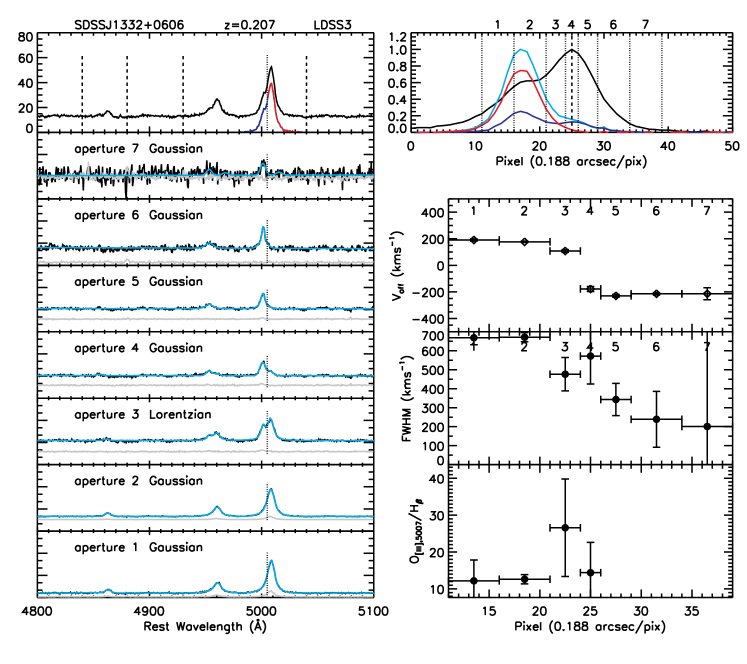
Figure 8: Diagnosis of the 2d spectrum of J1332+0606. Notation is the same as Fig. 3. The two velocity components are relatively well separated in space, and the stronger redshifted component has a larger line width than the weaker blueshifted component.

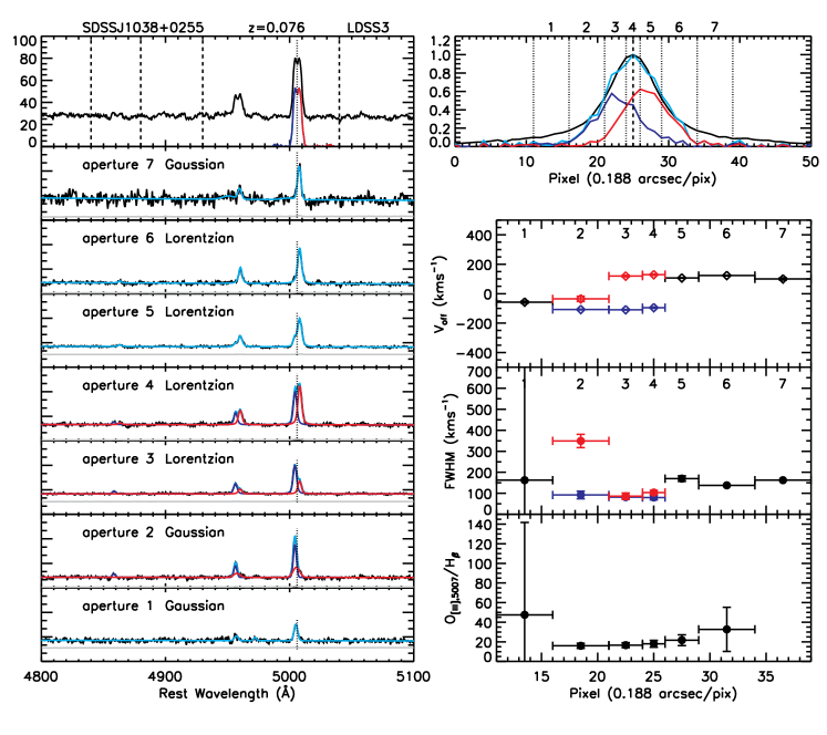
Figure 28: Diagnosis of the 2d spectrum of J1038+0255. Notation is the same as Fig. 3. Deblending of the two velocity components is not successful in over half the spatial bins.

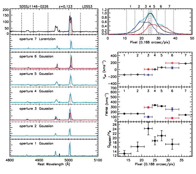
Figure 30: Diagnosis of the 2d spectrum of J1146$-$0226. Notation is the same as Fig. 3. Deblending is unsuccessful in the central bins as the velocity difference between the two components is too small there. This can be seen clearly in the 2d spectrum. The line width and the [O III]/H$\beta$ flux ratio seem to increase towards the center of the continuum, which is consistent with the ionizing source being at the center of the galaxy.

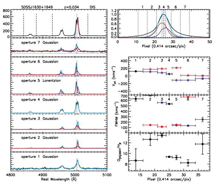
Figure 34: Diagnosis of the 2d spectrum of J1630+1649. Notation is the same as Fig. 3. Deblending of the two velocity components is ambiguous in most spatial bins. The [O III]/H$\beta$ flux ratio varies within $\sim 0.2$ dex.

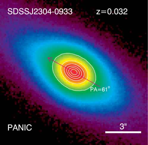
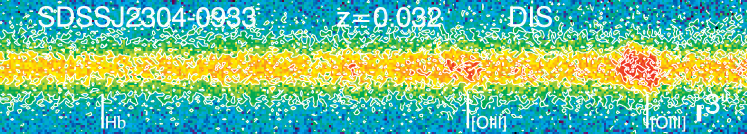
Figure 35: SDSS J2304$-$0933 (NLR kinematics). Upper: PANIC NIR image in $K_{s}$. This object has no resolved double nucleus, and a large disk component is apparent. Bottom: DIS 2d spectrum for the H$\beta$-[O III] region with corresponding lines marked (note that the locations of these line marks are approximate). The two velocity components are spatially offset by $\sim 0.8$″. Notation is the same as Fig. 2.

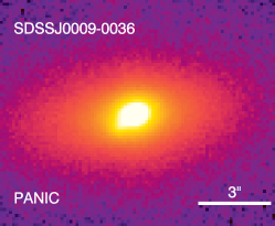
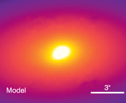
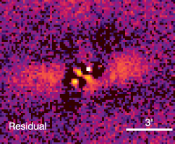
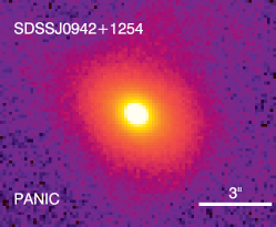
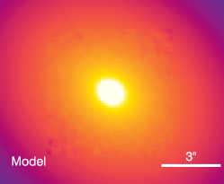
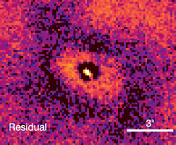
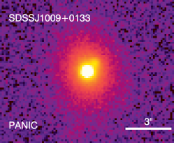
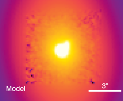
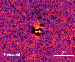
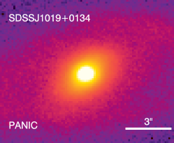
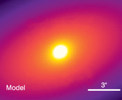
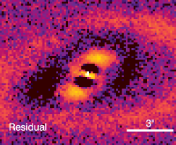
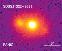
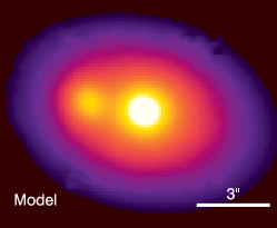
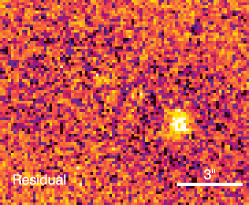
Figure 40: Model fits of the NIR surface brightness for objects classified as ambiguous cases (§3.3) using GALFIT. The first column shows the data, the second column shows the models and the last column shows the residuals. Note that the residual maps have been re-stretched to enhance the contrast and the residuals are not important compared to the observed fluxes (the apparent excess seen in some of the residual maps has values less than $5\%$ of the observed fluxes at the corresponding locations).

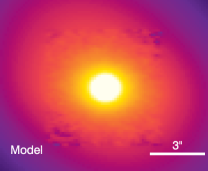
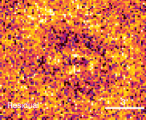
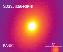
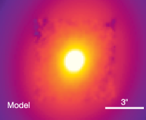
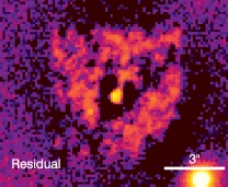
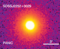
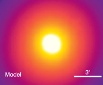
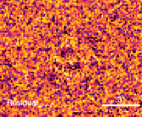
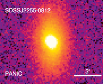
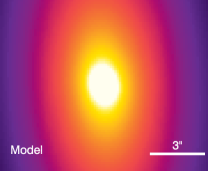
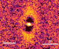
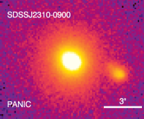
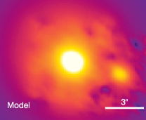
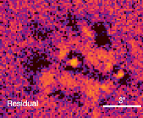
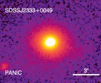
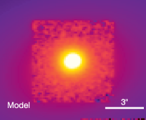
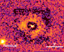
Figure 40: Continued.

References

- Baldwin et al. (1981) Baldwin, J. A., Phillips, M. M., & Terlevich, R. 1981, PASP, 93, 5
- Begelman et al. (1980) Begelman, M. C., Blandford, R. D., & Rees, M. J. 1980, Nature, 287, 307
- Bianchi et al. (2008) Bianchi, S., Chiaberge, M., Piconcelli, E., Guainazzi, M., & Matt, G. 2008, MNRAS, 386, 105
- Boroson & Lauer (2009) Boroson, T. A., & Lauer, T. R. 2009, Nature, 458, 53
- Civano et al. (2010) Civano, F., et al. 2010, ApJ, 717, 209
- Comerford et al. (2009a) Comerford, J. M., et al. 2009a, ApJ, 698, 956
- Comerford et al. (2009b) Comerford, J. M., Griffith, R. L., Gerke, B. F., Cooper, M. C., Newman, J. A., Davis, M., & Stern, D. 2009b, ApJ, 702, L82
- Crenshaw & Kraemer (2000) Crenshaw, D. M., & Kraemer, S. B. 2000, ApJ, 532, L101
- Crenshaw et al. (2000) Crenshaw, D. M., et al. 2000, AJ, 120, 1731
- Das et al. (2005) Das, V., et al. 2005, AJ, 130, 945
- Fischer et al. (2010) Fischer, T. C., Crenshaw, D. M., Kraemer, S. B., Schmitt, H. R., Mushotsky, R. F., & Dunn, J. P. 2010, ApJ, in press, arXiv:1011.4213
- Fu et al. (2010) Fu, H., Myers, A. D., Djorgovski, S. G., & Yan, L. 2010, arXiv:1009.0767
- Gerke et al. (2007) Gerke, B. F., et al. 2007, ApJ, 660, L23
- Greene et al. (2011) Greene, J. E., Zakamska, N. L., Ho, L. C., & Barth, A. J. 2011, ApJ, in press, arXiv:1102.2913
- Hamuy et al. (2006) Hamuy, M., et al. 2006, PASP, 118, 2
- Heckman et al. (1981) Heckman, T. M., Miley, G. K., van Breugel, W. J. M., & Butcher, H. R. 1981, ApJ, 247, 403
- Hennawi et al. (2010) Hennawi, J. F., et al. 2010, ApJ, 719, 1672
- Hennawi et al. (2006) —. 2006, AJ, 131, 1
- Hernquist (1989) Hernquist, L. 1989, Nature, 340, 687
- Hopkins et al. (2005) Hopkins, P. F., Hernquist, L., Martini, P., Cox, T. J., Robertson, B., Di Matteo, T., & Springel, V. 2005, ApJ, 625, L71
- Komossa et al. (2003) Komossa, S., Burwitz, V., Hasinger, G., Predehl, P., Kaastra, J. S., & Ikebe, Y. 2003, ApJ, 582, L15
- Liu et al. (2010a) Liu, X., Greene, J. E., Shen, Y., & Strauss, M. A. 2010a, ApJ, 715, L30
- Liu et al. (2010b) Liu, X., Shen, Y., Strauss, M. A., & Greene, J. E. 2010b, ApJ, 708, 427 (Paper I)
- Martini et al. (2004) Martini, P., Persson, S. E., Murphy, D. C., Birk, C., Shectman, S. A., Gunnels, S. M., & Koch, E. 2004, SPIE Conf., 5492, 1653
- Myers et al. (2008) Myers, A. D., Richards, G. T., Brunner, R. J., Schneider, D. P., Strand, N. E., Hall, P. B., Blomquist, J. A., & York, D. G. 2008, ApJ, 678, 635
- Peng et al. (2010) Peng, C. Y., Ho, L. C., Impey, C. D., & Rix, H.-W. 2010, AJ, 139, 2097
- Persson et al. (1998) Persson, S. E., Murphy, D. C., Krzeminski, W., Roth, M., & Rieke, M. J. 1998, AJ, 116, 2475
- Rodriguez et al. (2006) Rodriguez, C., Taylor, G. B., Zavala, R. T., Peck, A. B., Pollack, L. K., & Romani, R. W. 2006, ApJ, 646, 49
- Rosario et al. (2010) Rosario, D. J., Shields, G. A., Taylor, G. B., Salviander, S., & Smith, K. L. 2010, ApJ, 716, 131
- Rosario et al. (2011) Rosario, D. J., McGurk, R. C., Max, C. E., Shields, G. A. & Smith, K. L. 2011, arXiv:1102.1733
- Sargent (1972) Sargent, W. L. W. 1972, ApJ, 173, 7
- Sarzi et al. (2006) Sarzi, M., et al. 2006, MNRAS, 366, 1151
- Skrutskie et al. (2006) Skrutskie, M. F., et al. 2006, AJ, 131, 1163
- Smith et al. (2010) Smith, K. L., Shields, G. A., Bonning, E. W., McMullen, C. C., Rosario, D. J., & Salviander, S. 2010, ApJ, 716, 866
- Tody (1986) Tody, D. 1986, SPIE Conf., 627, 733
- Valtonen et al. (2008) Valtonen, M. J., et al. 2008, Nature, 452, 851
- Veilleux (1991) Veilleux, S. 1991, ApJS, 75, 357
- Veilleux et al. (2001) Veilleux, S., Shopbell, P. L., & Miller, S. T. 2001, AJ, 121, 198
- Wang et al. (2009) Wang, J., Chen, Y., Hu, C., Mao, W., Zhang, S., & Bian, W. 2009, ApJ, 705, L76
- Whittle et al. (2005) Whittle, M., Rosario, D. J., Silverman, J. D., Nelson, C. H., & Wilson, A. S. 2005, AJ, 129, 104
- Whittle & Wilson (2004) Whittle, M., & Wilson, A. S. 2004, AJ, 127, 606
- York et al. (2000) York, D. G., et al. 2000, AJ, 120, 1579
- Zhou et al. (2004) Zhou, H., Wang, T., Zhang, X., Dong, X., & Li, C. 2004, ApJ, 604, L33