The extended coupled cluster method and the pairing problem

Abstract

We study the application of various forms of the coupled cluster method to systems with paired fermions. The novel element of the analysis is the study of the breaking and eventual restoration of particle number in the CCM variants. We specifically include Arponen’s extended coupled cluster method, which describes the normal Hartree-Fock-Bogoliubov mean field at lowest level of truncation. We show that all methods converge to the exact results as we increase the order of truncation, but that the breaking of particle number at an intermediate level means that this convergence occurs in a surprising way. We argue that the most straightforward form of the method seems to be the most stable approach to implement for realistic (large number of particles) pairing problems

1 Introduction

The Coupled Cluster Method (CCM) has a long and venerable history in both Physics and Chemistry. It is a method that can be designed to incorporate the normal mean-field approximation, but in principle it also allows one to make systematic improvements, and in principle converges to the exact solution. After initial work by Coester and K mmel [1], and K mmel and his group [2] with important applications in nuclear physics, this was picked up in quantum chemistry by Čižek and Paldus [3, 4, 5, 6] and took off from there (see Ref. [7] for a recent review). About 10 years ago, the method made a renewed appearance in nuclear physics in the work of Mihaila and Heisenberg [8, 9, 10, 11], and in a more advanced application in the work of Dean et al [12, 13, 14, 15, 16, 17, 18, 19, 20, 21, 22]. Atomic nuclei are indeed interesting and complicated, even more so once we start thinking about heavier open shell nuclei, since we then have to take into account nuclear superfluidity, described by pairing of nucleons of opposite spins, as well as the “normal” problems of nuclear physics (short range repulsion, intermediate attraction, non-central forces). The normal way to deal with such nuclei using involves mean-field techniques, but one would like to use a fully microscopic method such as the CCM to tackle the full many-body problem, including the pairing part. Since we have some understanding of the nuclear physics complications, in this paper we shall concentrate on the pairing problem, to see how the CCM can be applied effectively to this aspect of the nuclear landscape.

Of course pairing is also extremely important in atomic (fermionic) condensates, where we have the added advantages that experimentalists can tune the $s$-wave scattering length, which determines the interaction in the pairing channel, to almost any value required [23]. This has allowed one to study the BEC to BCS transition, and has given many-body theory access to a whole new set of data that require an explanation. The extreme elegance and control of the experiments means that the data requires high accuracy calculations, and is also able to probe collective modes, some of which are beyond simple mean-field plus harmonic fluctuations (RPA) calculations. One technique that gives one easy access to such modes is again the CCM. This gives a second impetus to this study.

Little work has been done within CCM for problems with pairing forces. The so-called normal CCM has been used by Emrich and Zabolitzky [24, 25], but this work seems to have been largely forgotten, and it is probably not as general as required. If we are interested in systems with strong correlations, we may want to use methods that go beyond simple mean-field theory. The coupled cluster method has shown to be a very powerful technique to make such improvements, but we have little intuition what the best way to apply the method is. The work of Arponen [26] and Arponen and Bishop [27, 28, 29, 30, 31, 32] provides one way; the use of Brueckner/maximum overlap orbitals [33], where we start from the BCS wave function, and express all corrections in terms of BCS quasiparticles, is an alternative.

In this paper we shall investigate both these methods for a simplified model, with an emphasis on particle number–so we concentrate on a single one of the aspects that are important for finite nuclei. Before analyzing this model, let us first describe the methods used succinctly.

2 The normal CCM

Let us look at the traditional (normal) Coupled Cluster Method (NCCM) first, both to make contact with other notations used in the field, and for later reference.

We shall use the standard “Bochum/Manchester notation”, where $S$ denotes the cluster operator (called “$T$” in most chemically inspired literature). We also use the “SUB(n)” notation, where SUB(1) describes the truncation of the cluster operator to a single quasiparticle excitation, SUB(2) single plus double (SD), etc. Following Arponen [26], we start from a functional,

$$O(\tilde{s},s)=\langle\tilde{\phi}|O|\phi\rangle=\langle\phi_{0}|(1+\tilde{S})e^{-S}Oe^{S}|\phi_{0}\rangle,$$ (1)

which is used to evaluate the expectation value of any operator including the Hamiltonian. This has interesting linking properties: all $S$ operators contract with $O$, and the $\tilde{S}$ has to link with at least one $S$ or the $O$ operator.

The states used in the expectation value are not Hermitian conjugates, but are intermediate normalised,

$$\langle\phi_{0}|(1+\tilde{S})e^{-S}e^{S}|\phi_{0}\rangle=1.$$ (2)

The resulting expectation value is a finite polynomial once we impose the condition

$$S=\sum_{I}s_{I}C_{I}^{\dagger},\quad\tilde{S}=\sum_{I}\tilde{s}_{I}C_{I},$$ (3)

with the generalised annihilation operators

$$C_{I}\left|\phi_{0}\right\rangle=0.$$ (4)

The reason for the polynomial nature of the result is that the nested commutator expansion

$$e^{-S}Oe^{S}=O+[O,S]+\frac{1}{2!}[[O,S],S]+\ldots$$

terminates at finite order if the operator $O$ contains a finite number of operators.

Normal CCM is usually written in a slightly different form; if we extremise the energy (as expectation value of the Hamiltonian) with respect to $s_{I}$ and $\tilde{s}_{I}$, we only have to solve for $s_{I}$:

$$\langle\phi_{0}|C_{I}e^{-S^{\text{eq}}}He^{S^{\text{eq}}}|\phi_{0}\rangle = 0,$$ (5)

$$\langle\phi_{0}|e^{-S^{\text{eq}}}He^{S^{\text{eq}}}|\phi_{0}\rangle = E,$$ (6)

where we use “eq” to denote the equilibrium solution of (5). Of course to calculate the expectation value of any other operator we require $\tilde{s}_{I}^{\text{eq}}$ as well, which can be found from a set of inhomogeneous linear equations

$$\langle\phi_{0}|(1+\tilde{S}^{\text{eq}})e^{-S^{\text{eq}}}[H,C_{I}^{\dagger}]e^{S^{\text{eq}}}|\phi_{0}\rangle=0.$$

Finally, by expanding the action

$$\mathcal{A}[s,\tilde{s}]=\int dt\langle\tilde{\phi}|(1+\tilde{S})e^{-S}(H-i\partial_{t})e^{S}|\phi\rangle,$$ (7)

to second order about the equilibrium we get the “Harmonic approximation”, also called EOM-CC [34], with classical action, derived by shifting $s_{I}\rightarrow s_{I}^{\text{eq}}+s_{I}$

$$\mathcal{A} =\int\biggl{\{}i\sum_{I}(\tilde{s}_{I}+\tilde{s}^{\text{eq}})\dot{s}_{I}+\frac{1}{2}s_{I}s_{J}\left[\partial_{s_{I}}\partial_{s_{J}}H(s,\tilde{s}^{\text{eq}})|_{s=s^{\text{eq}}}\right]$$ (8)

$$+\tilde{s}_{I}s_{J}\left[\partial_{\tilde{s}_{I}}\partial_{s_{J}}H(s,\tilde{s})|_{s=s^{\text{eq}}}\right]\biggr{\}}dt.$$

(The linear term, a total derivative, is a boundary term and can thus normally be removed from the action.) Varying with respect to $\tilde{s}_{I}(t)$, assuming a harmonic dependence of $s_{I}$, $s_{I}=e_{I}e^{i\omega t}$, we get

$$\left[\partial_{\tilde{s}_{I}}\partial_{s_{J}}H(s,\tilde{s}^{\text{eq}})|_{s=s^{\text{eq}}}\right]e_{J}=\omega e_{I}\quad.$$ (9)

If we wish to get the tilde eigenstates as well, we need to vary with respect to $s_{J}(t)$, using $\tilde{s}_{I}=f_{i}e^{i\omega t}$

$$\left[\partial_{s_{I}}\partial_{s_{J}}H(s,\tilde{s}^{\text{eq}})|_{s=s^{\text{eq}}}\right]e_{J}+\left[\partial_{\tilde{s}_{J}}\partial_{s_{I}}H(s,\tilde{s}^{\text{ }})|_{s=s^{\text{eq}}}\right]f_{J}=-\omega f_{I}.$$ (10)

We can rewrite this as the eigenvectors of what looks like an RPA excited state problem [35] (which is due to the fact that this is the diagonalisation of a quadratic Hamiltonian)

$$\left(\begin{array}[]{cc}\partial_{s_{I}}\partial_{s_{J}}H(s,\tilde{s}^{\text{eq}})|_{s=s^{\text{eq}}}&\partial_{\tilde{s}_{J}}\partial_{s_{I}}H(s,\tilde{s}^{\text{ }})|_{s=s^{\text{eq}}}\\ \partial_{s_{J}}\partial_{\tilde{s}_{I}}H(s,\tilde{s})|_{s=s^{\text{eq}}}&0\end{array}\right){\boldsymbol{a}} = \left(\begin{array}[]{cc}0&-I\\ I&0\end{array}\right)\omega{\boldsymbol{a}},$$ (15)

where we have used the “double height column vector”

$${\boldsymbol{a}}=\left(\begin{array}[]{c}{\boldsymbol{e}}\\ {\boldsymbol{f}}\end{array}\right).$$ (16)

For this particular matrix the eigenvalues are completely determined by the diagonalisation of the lower left block $\partial_{s_{J}}\partial_{\tilde{s}_{I}}H(s,\tilde{s}^{\text{ }})|_{s=s^{\text{eq}}}$, which is the matrix of derivatives of the traditional CCM equations, which are given by the Eqs. (5), and are used to determine the coefficients $s_{I}$.

3 The extended CCM

The extended CCM starts from a similar functional as Eq. (1) , but now based on a double-exponential form of the bra states, [26]

$$O(\tilde{s},s)=\langle\tilde{\phi}|O|\phi\rangle=\langle\phi_{0}|e^{\tilde{S}}e^{-S}Oe^{S}|\phi_{0}\rangle.$$ (17)

The operators remain unchanged, i.e., they are defined in Eqs. (3) and (4). Unlike the ordinary NCCM, it has not been widely applied since it is much more difficult to evaluate. Here we discuss a quasiparticle approach that seems to hold some promise. We shall in essence make intimate use of a link to the theory of generalised coherent states, and the fact that Eq. (17) is identical to the Dyson-Maleev boson mapping of Lie algebras [36] when we can assign a Lie algebra to the operators $C_{I}$,$C_{I}^{\dagger}$ and their commutators.

When we minimize the energy, we can now no longer separate the steps in the determination of $s_{I}$ and $\tilde{s}_{I}$, but have to combine the equations

$$\langle\phi_{0}|C_{I}e^{\tilde{S}^{\text{eq}}}e^{-S^{\text{eq}}}He^{S^{\text{eq}}}|\phi_{0}\rangle = 0,$$

$$\langle\phi_{0}|e^{\tilde{S}^{\text{eq}}}e^{-S^{\text{eq}}}[H,C_{I}^{\dagger}]e^{S^{\text{eq}}}|\phi_{0}\rangle = 0,$$

$$\langle\phi_{0}|e^{\tilde{S}^{\text{eq}}}e^{-S^{\text{eq}}}He^{S^{\text{eq}}}|\phi_{0}\rangle = E.$$ (18)

Once we have solved these, we can look for the excited states by solving the harmonic problem, $s_{I}\rightarrow s_{I}^{\text{eq}}+s_{I}$, etc.,

$$\mathcal{A} = \int\biggl{\{}i\sum_{I}\langle\phi_{0}|e^{\tilde{S}}C_{I}^{\dagger}|\phi_{0}\rangle\dot{s}_{I}+\frac{1}{2}s_{I}s_{J}\left[\partial_{s_{I}}\partial_{s_{J}}H(s,\tilde{s}^{\text{eq}})|_{s=s^{\text{eq}}}\right]$$ (19)

$$+\tilde{s}_{I}s_{J}\left[\partial_{\tilde{s}_{I}}\partial_{s_{J}}H(s,\tilde{s}^{\text{eq}})|_{s=s^{\text{eq}}}\right]dt.\biggr{\}}$$

Varying with respect to $\tilde{s}_{I}(t)$, assuming a harmonic dependence of $s_{I}$, $s_{I}=e_{I}e^{i\omega t}$, we get

$$\left(\begin{array}[]{cc}\partial_{s_{I}}\partial_{s_{J}}H(s,\tilde{s})&\partial_{\tilde{s}_{J}}\partial_{s_{I}}H(s,\tilde{s}^{\text{ }})\\ \partial_{\tilde{s}_{I}}\partial_{s_{J}}H(s,\tilde{s})&\partial_{\tilde{s}_{I}}\partial_{\tilde{s}_{J}}H(s,\tilde{s})\end{array}\right)_{\text{eq}}{\boldsymbol{a}}=\mathcal{S}\omega{\boldsymbol{a}},$$ (22)

$$\mathcal{S}=\left(\begin{array}[]{cc}0&-\partial_{\tilde{s}_{J}}\left\langle\phi_{0}\right|e^{\tilde{S}}C_{I}^{\dagger}\left|\phi_{0}\right\rangle\\ \partial_{\tilde{s}_{I}}\left\langle\phi_{0}\right|e^{\tilde{S}}C_{J}^{\dagger}\left|\phi_{0}\right\rangle&0\end{array}\right)_{\text{eq}},$$ (25)

where the symplectic matrix $\mathcal{S}$ can be brought to canonical form by replacing the set of amplitudes $\{\tilde{s}_{J}\}$ by the new set $\{\sigma_{J}\}$ which solves the nonlinear equations

$$\sigma_{I}=\left\langle\phi_{0}\right|e^{\tilde{S}}C_{I}^{\dagger}\left|\phi_{0}\right\rangle,$$ (26)

and expanding the energy in these new amplitudes. This is not necessary to solve the RPA, however, and for certain mixed calculations (see below) such a transformation is not easily done, and we may want to choose to work with the form given in (22,25).

4 ECCM SUB(1) approximation and HFB

One of the natural ways to generalise the Hartree-Fock method to problems with pairing, and the BCS approach to problems with particle-hole interactions is the Hartree-Fock-Bogoliubov method. We still use a single Slater-determinant wave function, but the state has no definite particle number, like the BCS state. As shown below, we can capture this information in a generalised density matrix [35]. There is a CCM approximation that is equivalent to this state:

The ECCM SUB(1) approximation for a finite fermionic system, where the reference state is a single Slater determinant of occupied orbitals $h$

$$|\phi_{0}\rangle=\prod_{h}a_{h}^{\dagger}|0\rangle$$ (27)

is defined by the one-body $S$ operator

$$S=\sum_{ph}s^{ph}a_{p}^{\dagger}a_{h}+\sum_{pp^{\prime}}s^{pp^{\prime}}a_{p}^{\dagger}a_{p^{\prime}}^{\dagger}+\sum_{hh^{\prime}}s^{hh^{\prime}}a_{h^{\prime}}a_{h},$$ (28)

where $h$ labels the single-particle states occupied in the reference state, and $p$ the unoccupied ones. (In other words, this is the “singles” truncation of quantum chemistry, adapted to the pairing problem where we no longer preserve particle number). We now evaluate (17) by first using the nested commutator expansion for $e^{-S}He^{S}$. In calculating the commutator of $S$ with the Hamiltonian, either one or both of the operators in $S$ contract with $H$. If both contract, no further contractions are possible. Having performed all possible contractions with $S$ we need to now calculate the final contractions with $\tilde{S}$. In ECCM this will either tie together two $S$’s, one $S$ and link the other operator to $H$, or link both its indices to $H$. We thus get a factorisation of $S$ and $\tilde{S}$ into general objects with two external indices, essentially one-body densities, which is exactly the Hartree-Fock-Bogoliubov (HFB) factorisation, if we identify the linked strings of $S$ and $\tilde{S}$’s with the normal and abnormal densities. This can of course be made explicit: the algebra is rather lengthy, but see below for a simplified (BCS) example.

5 Simplifying SUB(1)

Let us look at the application of the extended CCM to a pure pairing problem (without particle-hole excitations) in the SUB1 approximation. We start from the standard definitions

$$S = \overbrace{\sum_{p}s_{p}a_{{\boldsymbol{p}}\uparrow}^{\dagger}a_{-{\boldsymbol{p}}\downarrow}^{\dagger}}^{S_{p}}+\overbrace{\sum_{h}s_{h}a_{{\boldsymbol{h}}\downarrow}a_{-{\boldsymbol{h}}\uparrow}}^{S_{h}},$$ (29)

$$\tilde{S} = \underbrace{\sum_{p}\tilde{s}_{p}a_{{\boldsymbol{p}}\downarrow}a_{-{\boldsymbol{p}}\uparrow}}_{\tilde{S}_{p}}+\underbrace{\sum_{h}\tilde{s}_{h}a_{{\boldsymbol{h}}\uparrow}^{\dagger}a_{-{\boldsymbol{h}}\downarrow}^{\dagger}}_{\tilde{S}_{h}}.$$ (30)

We also write

$$|\phi\rangle = e^{S}|\phi_{0}\rangle,\qquad\langle\tilde{\phi}|=\langle\phi_{0}|e^{\tilde{S}}e^{-S}\quad.$$ (31)

We now analyse the normal and abnormal densities [35] in the standard way.

The normal density $\rho_{i\sigma,j\sigma^{\prime}}=\langle\tilde{\phi}|a_{{\boldsymbol{j}}\sigma^{\prime}}^{\dagger}a_{{\boldsymbol{i}}\sigma}|\phi\rangle$ equals

$$\rho_{i\sigma,j\sigma^{\prime}}=\delta_{\sigma\sigma^{\prime}}\left[\sum_{{\boldsymbol{h}}}\delta_{{\boldsymbol{i}}{\boldsymbol{j}}}^{h}\left(1-\tilde{s}_{h}s_{h}\right)+\sum_{{\boldsymbol{p}}}\delta_{{\boldsymbol{i}}{\boldsymbol{j}}}^{p}\tilde{s}_{p}s_{p}\right]\quad,$$ (32)

and the abnormal densities require a bit more work, but after some algebra can be expressed as

$$\kappa_{{\boldsymbol{i}}\sigma,{\boldsymbol{j}}\sigma^{\prime}} = \langle\tilde{\phi}|a_{{\boldsymbol{j}}\sigma^{\prime}}a_{{\boldsymbol{i}}\sigma}|\phi\rangle$$ (33)

$$= \left[\delta_{\sigma\uparrow}\delta_{\sigma^{\prime}\downarrow}-\delta_{\sigma\downarrow}\delta_{\sigma^{\prime}\uparrow}\right]\left\{\tilde{s}_{h}\delta_{{\boldsymbol{i}},\bar{{\boldsymbol{j}}}}^{h}+s_{p}(1-s_{p}\tilde{s}_{p})\delta_{{\boldsymbol{i}},\bar{{\boldsymbol{j}}}}^{p}\right\}.$$

The bar denotes the time-reversed state

5.1 Generalised density

From the standard block-matrix definition of the generalised density,

$$\mathcal{R}=\left(\begin{array}[]{cc}\rho&\kappa\\ -\kappa^{*}&I-\rho^{*}\end{array}\right),$$ (34)

we can easily check that $\mathcal{R}^{2}=\mathcal{R}$. Expanding out this projector condition, we get the four matrix conditions

$$\rho^{2}-\kappa\,\kappa^{*} = \rho,$$

$$\rho\kappa-\kappa\rho^{*} = 0,$$

$$\rho^{*}\kappa^{*}-\kappa^{*}\rho = 0,$$

$$\rho^{*2}-\kappa^{*}\kappa = \rho^{*}.$$ (35)

Let us show explicitly how one of these works for the forms found above. First notice that

$$\left[\delta_{\sigma\uparrow}\delta_{\sigma^{\prime}\downarrow}-\delta_{\sigma\downarrow}\delta_{\sigma^{\prime}\uparrow}\right]\left[\delta_{\sigma^{\prime}\uparrow}\delta_{\sigma^{\prime\prime}\downarrow}-\delta_{\sigma^{\prime}\downarrow}\delta_{\sigma^{\prime\prime}\uparrow}\right] = -\delta_{\sigma\uparrow}\delta_{\sigma^{\prime\prime}\uparrow}-\delta_{\sigma\downarrow}\delta_{\sigma^{\prime\prime}\downarrow}=-\delta_{\sigma\sigma^{\prime\prime}}\quad.$$ (36)

Thus

$$\rho^{2} = \delta_{\sigma\sigma^{\prime}}\left[\sum_{{\boldsymbol{h}}}\delta_{{\boldsymbol{i}}{\boldsymbol{j}}}^{h}\left(1-\tilde{s}_{h}s_{h}\right)^{2}+\sum_{{\boldsymbol{p}}}\delta_{{\boldsymbol{i}}{\boldsymbol{j}}}^{p}(\tilde{s}_{p}s_{p})^{2}\right]$$

$$-\kappa\kappa^{*} = \delta_{\sigma\sigma^{\prime}}\left[\sum_{{\boldsymbol{h}}}\delta_{{\boldsymbol{i}}{\boldsymbol{j}}}^{h}\left(1-\tilde{s}_{h}s_{h}\right)\tilde{s}_{h}s_{h}+\sum_{{\boldsymbol{p}}}\delta_{{\boldsymbol{i}}{\boldsymbol{j}}}^{p}(\tilde{s}_{p}s_{p})\left(1-\tilde{s}_{p}s_{p}\right)\right]$$ (37)

which add up to $\rho$.

Of course, the other three elements can be evaluated in a similar way. This shows that we have a general non-Hermitian classical mapping of the general density matrix.

[Discuss mapping issues]

5.2 Canonical form

In the literature (e.g., Ref. [35]) we can find the canonical form for the density matrix as

$$\rho = v_{p}^{2}\delta_{{\boldsymbol{p}},{\boldsymbol{p}}^{\prime}}+u_{h}^{2}\delta_{{\boldsymbol{h}},{\boldsymbol{h}}^{\prime}},$$ (38)

$$\kappa = \kappa^{*}=u_{k}v_{k}\delta_{{\boldsymbol{k}},\overline{{\boldsymbol{k}}^{\prime}}}.$$ (39)

Our expressions should be of the same form, since we have assumed the diagonal form of $S$. Actually, we pay a price here for unnecessarily starting with a Hartree-Fock state; all calculations above are valid with respect to the vacuum as well, where we recover a simpler form of BCS (which has maximal asymmetry of $\kappa$!). From the relations

$$\rho = v_{k}^{2}\left(\delta_{{\boldsymbol{k}},{\boldsymbol{k}}^{\prime}}+\delta_{\overline{{\boldsymbol{k}}},\overline{{\boldsymbol{k}}^{\prime}}}\right),$$ (40)

$$\kappa = \kappa^{*}=u_{k}v_{k}\delta_{{\boldsymbol{k}},\overline{{\boldsymbol{k}}^{\prime}}},$$ (41)

where we have rewritten the basis as

$${\boldsymbol{k}}={\boldsymbol{k}}\uparrow,\qquad\overline{{\boldsymbol{k}}}=-{\boldsymbol{k}}\downarrow,$$ (42)

we thus conclude that

$$\tilde{s}_{k} = v_{k}u_{k}=\frac{1}{2}\sin 2\psi_{k},$$ (43)

$$s_{k} = v_{k}/u_{k}=\cot\psi_{k}.$$ (44)

The energy, which is equal to the BCS energy, and is thus fully variational, is

$$I(s,\tilde{s})=2\epsilon_{k}s_{k}\tilde{s}_{k}+v_{k_{1}k_{2}k_{1}k_{2}}s_{k_{1}}\tilde{s}_{k_{1}}s_{k_{2}}\tilde{s}_{k_{2}}+v_{k_{2}k_{2}k_{1}k_{1}}s_{k_{1}}\left(1-s_{k_{1}}\tilde{s}_{k_{1}}\right)\tilde{s}_{k_{2}}.$$ (45)

This needs to be extended with a Lagrange multiplier for particle number–since we break particle number we need to make sure that at least the average particle number is correct. At this level if truncation, we get a term $-\lambda\left(s_{k}\tilde{s}_{k}-N_{0}\right)$ in the functional.

[Needs to be mentioned earlier as well]

5.3 Quasiparticle basis

It is interesting to note that the parametrisation above is naturally linked to a bi-canonical operatorial basis ($c^{\dagger}\neq d^{\dagger}$, but $\{d_{{\boldsymbol{k}}}^{\dagger},c_{{\boldsymbol{l}}}\}=\delta_{{\boldsymbol{k}},{\boldsymbol{l}}}$), which is obtained by calculating the action of $a_{k}$ on the ket $|\phi\rangle$ and $a_{k}^{\dagger}$ on the bra $\langle\tilde{\phi}|$ (the idea to use bi-canonical operators traces back at least as far as Ref. [37]), in each case subtracting the result from the initial operator:

$$c_{{\boldsymbol{k}}} = a_{{\boldsymbol{k}}}+\left[S,a_{{\boldsymbol{k}}}\right]=a_{{\boldsymbol{k}}}-s_{k}a_{\overline{{\boldsymbol{k}}}}^{\dagger},$$

$$c_{\overline{{\boldsymbol{k}}}} = a_{\overline{{\boldsymbol{k}}}}+\left[S,a_{\bar{{\boldsymbol{k}}}}\right]=a_{\overline{{\boldsymbol{k}}}}+s_{k}a_{{\boldsymbol{k}}}^{\dagger},$$

$$d_{{\boldsymbol{k}}}^{\dagger} = a_{{\boldsymbol{k}}}^{\dagger}+\left[\tilde{S},a_{{\boldsymbol{k}}}^{\dagger}\right]+\left[S,\left[\tilde{S},a_{{\boldsymbol{k}}}^{\dagger}\right]\right]=(1-\tilde{s}_{k}s_{k})a_{{\boldsymbol{k}}}^{\dagger}-\tilde{s}_{k}a_{\overline{{\boldsymbol{k}}}},$$

$$d_{\overline{{\boldsymbol{k}}}}^{\dagger} = a_{\overline{{\boldsymbol{k}}}}^{\dagger}+\left[\tilde{S},a_{\overline{{\boldsymbol{k}}}}^{\dagger}\right]+\left[S,\left[\tilde{S},a_{\overline{{\boldsymbol{k}}}}^{\dagger}\right]\right]=(1-\tilde{s}_{k}s_{k})a_{\overline{{\boldsymbol{k}}}}^{\dagger}+\tilde{s}_{k}a_{{\boldsymbol{k}}}.$$ (46)

This can be inverted to give

$$a_{{\boldsymbol{k}}} = (1-\tilde{s}_{k}s_{k})c_{{\boldsymbol{k}}}+s_{k}d_{\overline{{\boldsymbol{k}}}}^{\dagger},$$

$$a_{\overline{{\boldsymbol{k}}}} = (1-\tilde{s}_{k}s_{k})c_{\overline{{\boldsymbol{k}}}}-s_{k}d_{{\boldsymbol{k}}}^{\dagger},$$

$$a_{{\boldsymbol{k}}}^{\dagger} = \tilde{s}_{k}c_{\overline{{\boldsymbol{k}}}}+d_{{\boldsymbol{k}}}^{\dagger},$$

$$a_{\overline{{\boldsymbol{k}}}}^{\dagger} = -\tilde{s}_{k}c_{{\boldsymbol{k}}}+d_{\overline{{\boldsymbol{k}}}}^{\dagger}.$$ (47)

Using these relations we can transform the original Hamiltonian (there is no sum over spin indices, since we have chosen a Hamiltonian with $S$-wave pairing only):

$$H=\sum_{{\boldsymbol{k}},\sigma}\epsilon_{k}n_{{\boldsymbol{k}},\sigma}+\sum_{k_{1}k_{2}k_{3}k_{4}}v_{k_{1}k_{2}k_{3}k_{4}}a_{{\boldsymbol{k}}_{1}}^{\dagger}a_{\overline{{\boldsymbol{k}}}_{2}}^{\dagger}a_{\overline{{\boldsymbol{k}}}_{4}}a_{{\boldsymbol{k}}_{3}}.$$ (48)

If we use a time-reversal invariant potential, $v_{k_{1}k_{2}k_{3}k_{4}}=v_{k_{3}k_{4}k_{1}k_{2}}$, and we also assume spin-balance, $v_{k_{1}k_{2}k_{3}k_{4}}=v_{k_{2}k_{1}k_{4}k_{3}},$ we have

$$H^{\text{qp}} = H^{0}+H_{k}^{20}d_{{\boldsymbol{k}}}^{\dagger}d_{\overline{{\boldsymbol{k}}}}^{\dagger}+H_{k}^{20}c_{\overline{{\boldsymbol{k}}}}c_{{\boldsymbol{k}}}+H_{k}^{11}d_{{\boldsymbol{k}}}^{\dagger}c_{{\boldsymbol{k}}}+H_{\bar{k}}^{11}d_{\overline{{\boldsymbol{k}}}}^{\dagger}c_{\overline{{\boldsymbol{k}}}}$$ (49)

$$+ H_{k_{1}k_{2}k_{3}k_{4}}^{40}d_{{\boldsymbol{k}}_{1}}^{\dagger}d_{{\boldsymbol{k}}_{2}}^{\dagger}d_{\overline{{\boldsymbol{k}}}_{3}}^{\dagger}d_{\overline{{\boldsymbol{k}}}_{4}}^{\dagger}+H_{k_{1}k_{2}k_{3}k_{4}}^{04}c_{\overline{{\boldsymbol{k}}}_{1}}c_{\overline{{\boldsymbol{k}}}_{2}}c_{{\boldsymbol{k}}_{3}}c_{{\boldsymbol{k}}_{4}}$$

$$+ H_{k_{1}k_{2}\overline{k}_{3}k_{4}}^{31}d_{{\boldsymbol{k}}_{1}}^{\dagger}d_{{\boldsymbol{k}}_{2}}^{\dagger}d_{\overline{{\boldsymbol{k}}}_{3}}^{\dagger}c_{{\boldsymbol{k}}_{4}}+H_{k_{1}\overline{k}_{2}\overline{k}_{3}\overline{k}_{4}}^{31}d_{{\boldsymbol{k}}_{1}}^{\dagger}d_{\overline{{\boldsymbol{k}}}_{2}}^{\dagger}d_{\overline{{\boldsymbol{k}}}_{3}}^{\dagger}c_{\overline{{\boldsymbol{k}}}_{4}}$$

$$+ H_{k_{1}\overline{k}_{2}k_{3}k_{4}}^{13}d_{{\boldsymbol{k}}_{1}}^{\dagger}c_{\overline{{\boldsymbol{k}}}_{2}}c_{{\boldsymbol{k}}_{3}}c_{{\boldsymbol{k}}_{4}}+H_{\overline{k}_{1}\overline{k}_{2}\overline{k}_{3}k_{4}}^{13}d_{\overline{{\boldsymbol{k}}}_{1}}^{\dagger}c_{\overline{{\boldsymbol{k}}}_{2}}c_{\overline{{\boldsymbol{k}}}_{3}}c_{{\boldsymbol{k}}_{4}}$$

$$+ H_{k_{1}k_{2}k_{3}k_{4}}^{22}d_{{\boldsymbol{k}}_{1}}^{\dagger}d_{{\boldsymbol{k}}_{2}}^{\dagger}c_{{\boldsymbol{k}}_{3}}c_{{\boldsymbol{k}}_{4}}+H_{\overline{k}_{1}\overline{k}_{2}\overline{k}_{3}\overline{k}_{4}}^{22}d_{\overline{{\boldsymbol{k}}}_{1}}^{\dagger}d_{\overline{{\boldsymbol{k}}}_{2}}^{\dagger}c_{\overline{{\boldsymbol{k}}}_{3}}c_{\overline{{\boldsymbol{k}}}_{4}}$$

$$\qquad+H_{k_{1}\overline{k}_{2}\overline{k}_{3}k_{4}}^{22}d_{{\boldsymbol{k}}_{1}}^{\dagger}d_{\overline{{\boldsymbol{k}}}_{2}}^{\dagger}c_{\overline{{\boldsymbol{k}}}_{3}}c_{{\boldsymbol{k}}_{4}},$$

which is the non-Hermitian analogue of the standard quasiparticle Hamiltonian [35]. As the normal quasiparticle Hamiltonian, it can be used to simplify calculations.

5.4 Higher order terms and Brueckner orbitals

Of course we can calculate higher order CCM contributions as well; see below for some explicit examples. In general, one of the main problems in applying the extended CCM in this way is the proliferation of terms (“diagrams”) containing $S^{(1)}$ contributions–these describe the rotation of any single particle state, external or internal, whereas in NCCM we only rotate external states. One way to avoid this proliferation, is to use the quasiparticle Hamiltonian (49) defined above, and express the correlation through an $S^{(2)}$ operator expressed in the quasiparticles–or for that fact an even higher-order operator–

$$S^{(2)}=s_{k_{1}k_{2}k_{3}k_{4}}^{(2)}d_{{\boldsymbol{k}}_{1}}^{\dagger}d_{{\boldsymbol{k}}_{2}}^{\dagger}d_{\overline{{\boldsymbol{k}}}_{3}}^{\dagger}d_{\overline{{\boldsymbol{k}}}_{4}}^{\dagger},\qquad\tilde{S}^{(2)}=\tilde{s}_{k_{1}k_{2}k_{3}k_{4}}^{(2)}c_{\overline{{\boldsymbol{k}}}_{1}}c_{\overline{{\boldsymbol{k}}}_{2}}c_{{\boldsymbol{k}}_{3}}c_{{\boldsymbol{k}}_{4}},$$ (50)

i.e.

$$I(s^{(2)},\tilde{s}^{(2)},s,\tilde{s})=\left\langle\tilde{\phi}\right|\left\{\begin{array}[]{c}e^{\tilde{S}^{(2)}}\\ 1+\tilde{S}^{(2)}\end{array}\right\}e^{-S^{(2)}}H^{\text{qp}}e^{S^{(2)}}\left|\phi\right\rangle.$$ (51)

where the alternative shows that we can have either ECCM or NCCM for the extra terms. This corresponds to the use of what is called “Brueckner orbitals” in Quantum Chemistry, as long as we optimize the quasiparticle operators and the $S^{(n)}$, $n>2$, at the same time. Since the inclusion of higher order terms is our main target, we shall look specifically at these two methods.

6 Single shell pairing

6.1 Model investigation

In order to analyse the various approaches, we study a model. The simplest model exhibiting many of the features we are interested in, is the single-shell pairing model. This has a Hamiltonian of the form [35]

$$H=-G(\Delta^{\dagger}\Delta-N/2).$$ (52)

In the context used here, we interpret it as describing $\Omega$ states, each with spin up or down. In both cases we can divide the states into two equal size sets labeled by $k$ and $\bar{k}$, which are then paired,

$$\Delta^{\dagger} = \sum_{k=1}^{\Omega}a_{k}^{\dagger}a_{\bar{k}}^{\dagger},$$

$$N = \sum_{k=1}^{\Omega}a_{k}^{\dagger}a_{k}+\sum_{k=1}^{\Omega}a_{\bar{k}}^{\dagger}a_{\bar{k}}.$$ (53)

These operators form the well-known SI(2) quasispin algebra [35]

$$[\Delta,\Delta^{\dagger}] = 2(\Omega/2-N/2)\equiv 2J_{0},$$

$${}[J_{0},\Delta^{\dagger}] = -\Delta^{\dagger},$$ (54)

$${}[J_{0},\Delta] = \Delta.$$

From the algebra, we can easily derive the result that the non-degenerate ground state for even particle number $N$ is the state $\Delta^{\dagger N/2}|0\rangle$, and the energy of this groundstate is

$$E_{N}=-G\left(\Omega-\frac{N}{2}\right)\frac{N}{2}.$$ (55)

6.2 CCM

In order to find the coupled-cluster approximation to the exact solution, we need to find the extremum of the constrained energy

$$E(s,\tilde{s})=\langle 0|e^{-\tilde{S}}e^{S}\left[H-\lambda(N-N_{0})\right]e^{S}|0\rangle.$$ (56)

We find to lowest order that $s$ cannot depend on the magnetic quantum number, since there is no preferred direction, and thus

$$E(s,\tilde{s})=-\lambda\left(2\Omega s\tilde{s}-N_{0}\right)-G\Omega(\Omega-1)s\tilde{s}(1-s\tilde{ns}).$$

Isolating the chemical potential term, we see that

$$2\Omega s\tilde{s}=\left\langle N\right\rangle=N_{0},$$ (57)

and thus

$$s\tilde{s}=\frac{N_{0}}{2\Omega}.$$ (58)

We see a generic feature of the problem emerging: since we cast a variational calculation as a bi-variational one, introducing superfluous variables, there is no unique solution to $s$ and $\tilde{s}$ separately. The standard choice would be

$$\left\langle\Delta\right\rangle=\left\langle\Delta^{\dagger}\right\rangle,$$ (59)

where we find

$$s = \sqrt{\frac{N_{0}}{2\Omega-n}},$$

$$\tilde{s} = \sqrt{\frac{N_{0}(2\Omega-N_{0})}{(2\Omega)^{2}}},$$ (60)

but it is not necessary to make this choice. The SUB(1) approximation to the ground-state energy is thus

$$E=-G\frac{N_{0}}{2}\frac{\Omega-1}{\Omega}\left(\Omega-\frac{N_{0}}{2}\right),$$ (61)

which up to the correction of relative order $1/\Omega$ is the exact answer.

6.2.1 “Particle” ECCM

We shall first study the ECCM based on the normal (“particle”) operators, which, although normally a very lengthy calculation, is a simple calculation for this model, since we can use the quasispin algebra (54) to work out all results. In light of the fact that the exact solutions are of the form $\Delta^{\dagger N/2}|0\rangle$, we shall only consider the limited set of CCM states with structure

$$|\Phi\rangle=\exp\left(\sum_{n=1}^{M}s_{n}\Delta^{\dagger n}\right)|0\rangle.$$ (62)

We have performed calculations with $M$ up to 7.

6.2.2 Quasiparticle ECCM

The quasiparticle Hamiltonian is quite simple in this case. We use the quasiparticle number operator $n=d_{k}^{\dagger}c_{k}+d_{\bar{k}}^{\dagger}c_{\bar{k}}$, and the quasiparticle pair operators $\delta=c_{\bar{k}}c_{k}$ and $\delta^{\dagger}=d_{k}^{\dagger}d_{\bar{k}}^{\dagger}$ to write

$$H/G= \Omega /2-(1-s\tilde{s})s\tilde{s}(\Omega-n)^{2}$$ (63)

$$+ \left[(1-s\tilde{s})^{2}+(s\tilde{s})^{2}\right]\left[\delta^{\dagger}\delta-(\Omega-n)/2\right]$$

$$+ s^{2}\delta^{\dagger}\delta^{\dagger}+\left[\tilde{s}(1-s\tilde{s})\right]^{2}\delta\delta$$

$$- s(1-2s\tilde{s})\delta^{\dagger}(\Omega-n-1)-\tilde{s}(1-s\tilde{s})(1-2s\tilde{s})(\Omega-n-1)\delta.$$

At the same time

$$N = -(1-2s\tilde{s})(\Omega-n)+\Omega-2s\delta^{\dagger}-2\tilde{s}(1-s\tilde{s})\delta,$$ (64)

and

$$N^{2}= \Omega^{2} +4\Omega s\delta^{\dagger}+4\Omega\tilde{s}(1-s\tilde{s})\delta$$ (65)

$$+ 8(1-s\tilde{s})s\tilde{s}\delta^{\dagger}\delta$$

$$+ (1-2s\tilde{s})^{2}(\Omega-n)^{2}+2(2s\tilde{s}(1-s\tilde{s})-(1-2s\tilde{s})\Omega)(\Omega-n)$$

$$+ 4s^{2}\delta^{\dagger}\delta^{\dagger}+4\left[\tilde{s}(1-s\tilde{s})\right]^{2}\delta\delta$$

$$- 4s(1-2s\tilde{s})\delta^{\dagger}(\Omega-n-1)-4\tilde{s}(1-s\tilde{s})(1-2s\tilde{s})(\Omega-n-1)\delta.$$

We now calculate the expectation value of $H-\lambda N$ in the more general state

$$\langle\tilde{-}|e^{\tilde{S}^{(M)}}e^{-S^{(M)}}\left(H-\lambda N\right)e^{S^{(M)}}|-\rangle.$$ (66)

where we use the SUB($M$) approximation,

$$S^{(M)}=\sum_{n=2}^{M}\frac{1}{n!}s^{(n)}\left(\delta^{\dagger}\right)^{n},\quad\tilde{S}^{(M)}=\sum_{n=2}^{M}\frac{1}{n!}\tilde{s}^{(n)}\delta^{n},$$ (67)

and

$$|-\rangle=e^{S^{(1)}}\left|0\right\rangle,\quad\langle\tilde{-}|=\langle\tilde{0}|e^{\tilde{S}^{(1)}}e^{-S^{(1)}}.$$ (68)

All relevant commutators can easily be done using the quasiparticle quasispin algebra,

$$[\delta,(\delta^{\dagger})^{m}] = (\delta^{\dagger})^{m-1}(\Omega-n-m-1),$$

$${}[n,(\delta^{\dagger})^{m}] = 2m(\delta^{\dagger})^{m},$$

$${}[\delta n,(\delta^{\dagger})^{m}] = m(\delta^{\dagger})^{m-1}(\Omega-n-m+1)(n+2m)+2m(\delta^{\dagger})^{m}\delta,$$

$${}[\delta^{2},(\delta^{\dagger})^{m}] = m(m-1)(\delta^{\dagger})^{m-2}(\Omega-n-m+2)(\Omega-n-m+1)$$

$$+2m(\delta^{\dagger})^{m-1}\delta(\Omega-n-m+2).$$

Finally we need

$$\langle\tilde{-}|e^{\tilde{S}}(\delta^{\dagger})^{l}|-\rangle=\prod_{n=2}\delta_{\sum_{m=2}mk_{m},l}\frac{\left(\tilde{s}^{(n)}\right)^{k_{n}}}{k_{n}!}\frac{l!\Omega!}{(\Omega-l!)}.$$ (69)

6.3 Results

6.3.1 ECCM based on particles

We first wish to analyse the convergence of the ECCM based on the original operators. This has two reasons. First of all this will be a good test of the technology used in the implementation of the equations, which are all based on the algebraic implementation of the quasispin algebra–we shall see below why this is important. Also, we would like to understand what type of solutions we get, and how we approach the exact solution.

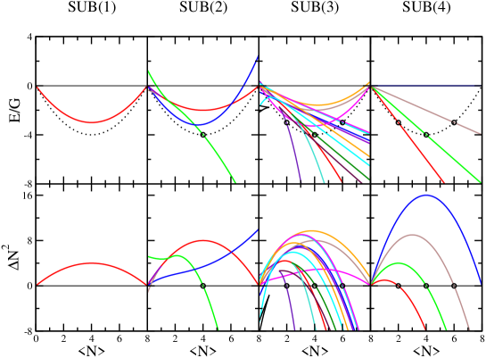
Figure 1: A plot of the energy (upper panels) and the fluctuation in particle number (lower panels) for SUB(1) to SUB(4) ECCM based on the particle picture, for $\Omega=4$. Black circles denote an exact solution.

With the help of Mathematica, we can obtain the full solution to the CCM equations, i.e., all real solutions to the coupled polynomial equations, see Fig. 1. As we increase the truncation from the SUB(1) level–which is just the normal BCS approximation– to the SUB(2) level we see some new solutions appearing. The green line, which is not a very good solution in most cases, is actually exact at half filling. The blue line is a better approximation than BCS up to about half filling. The SUB(3) results give a rather busy picture, with lots of solutions, among which are exact solutions (for $N=0,2,4,6,8$). Finally for SUB(4), where ECCM coincides with NCCM, we find exactly four branches of the solution, but each physical solution lies on a different branch. Also, all of these solutions are infinitely degenerate; something which is not obvious from the diagrams! This should not surprise us: in the SUB(4) calculation each of these states is orthogonal to the reference state, and is (essentially) generated by a single $\Delta^{\dagger n}$ excitation on the ground state.

In general we can prove that

$$\langle H\rangle=\frac{1}{4}\langle N^{2}\rangle-\frac{\Omega}{2}\langle N\rangle.$$ (70)

Putting in the explicit form of the ground state energy, we can show that a state where the expectation value of $H$ is the ground-state energy is also a state where $\langle N^{2}\rangle=\langle N\rangle^{2}$, i.e., $\Delta N^{2}=0$.

It should worry us that the usual implicit assumption in CCM–that the physical solution is smoothly connected in parameter space–is not correct in this case. If we are interested in a relatively low order SUB($n$) calculation for a problem with many particles this may not be such an important problem, but this requires detailed investigation.

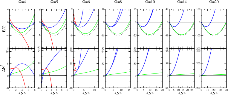
Figure 2: A plot of the energy (upper panels) and the fluctuation in particle number for SUB(2) ECCM based on the particle picture, for a variety of values of the degeneracy $\Omega$.

Notwithstanding those concerns, if we apply the SUB(2) ECCM to a variety of values of $\Omega$, see Fig. 2, we see that this is quite a successful and stable improvement to the BCS below the half-filled shell. Above that we could work with holes relative to the full shell and get much better results.

We can now concentrate on the “physical branch” of solutions, identified by the smooth connection to the ground state, and use solution following techniques to trace the higher order solutions for this value. In other word, we only solve a small subset. We choose $\Omega=10$, and find the result of Fig. 3. We see that we can indeed improve the results considerably, but also note the indication that there is a limit to the improvement. This is obvious from the fact that we know this is not the exact solution as we increase the truncation level.

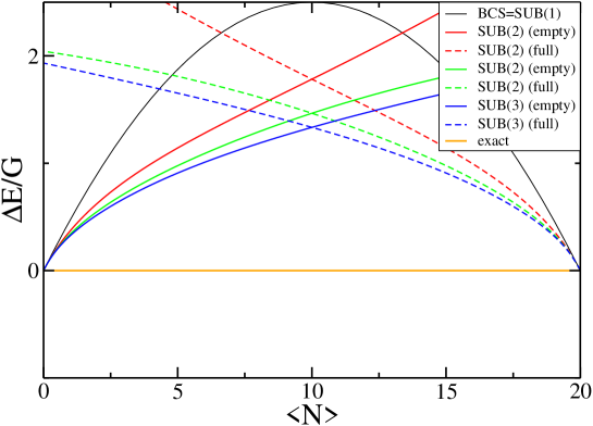
Figure 3: A plot $\Delta E=E-E_{\text{exact}}$ vs $\langle N\rangle$ for $\Omega=10$ using ECCM, with “ordinary” operators, rather than quasiparticle ones. We compare different levels of truncation, with either hole operators acting on the completely filled state (full) or particle operators acting on the empty state.

6.3.2 Brueckner orbitals

We would like to analyse the same systems for the quasiparticle ECCM (and NCCM). Unfortunately getting a full set of solutions to the quasiparticle ECCM, even for $\Omega=4$, as in Fig. 1 has proven to be impossible-the equations are just too complicated to get a complete set of solutions beyond SUB(2). If we look at the quasiparticle NCCM and ECCM for the SUB(2) case (only $s^{(2)}$ and $\tilde{s}^{(2)}$are non-zero) we get a rather interesting looking set of solutions, see Fig. 6.

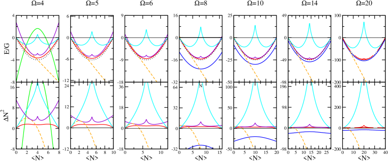
Figure 4: A plot of the energy (upper panels) and the fluctuation in particle number (lower panel) for SUB(2) quasiparticle NCCM based on the quasiparticle picture, for a variety of values of the degeneracy $\Omega$.

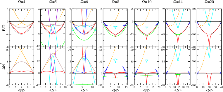
Figure 5: A plot of the energy (upper panels) and the fluctuation in particle number for SUB(2) quasiparticle ECCM based on the quasiparticle picture, for a variety of values of the degeneracy $\Omega$.

In that figure we see the usual multitude of solutions; the physically correct one (that turns to $E=0$ for $\langle N\rangle=0$) collapses at mid-shell. This agrees with the fact that $\Delta N^{2}$ goes negative around midshell, showing this is or has become an unphysical solution. Doing the same calculation with NCCM for the $S^{(2)}$ operators gives a better result, to our great surprise.

If we increase the order of the calculation, we see a suggestion of convergence for the odd (but not even orders).

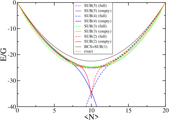
Figure 6: A plot $E$ as a function of $\langle N\rangle$ for $\Omega=10$, using the quasispin ECCM. We compare different levels of truncation, with either the filled (full) or empty state as a reference state.

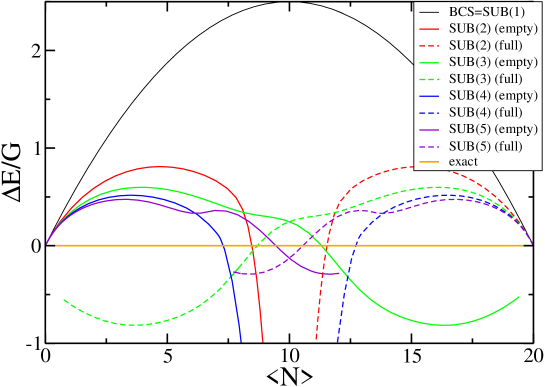
Figure 7: A plot $\Delta E=E-E_{\text{exact}}$ vs $\langle N\rangle$ for $\Omega=10$ , using the quasispin ECCM. We compare different levels of truncation, with either the filled (full) or empty state as a reference state.

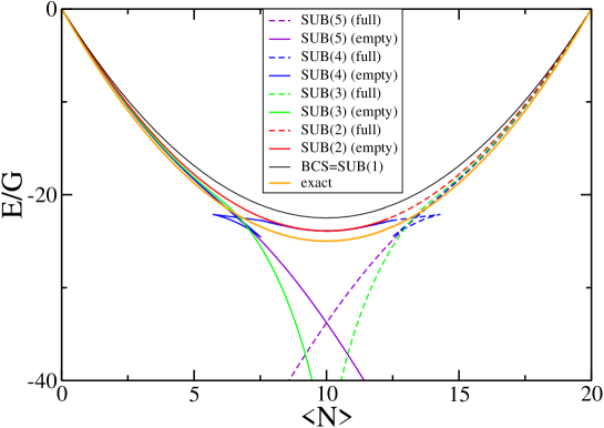
Figure 8: A plot $E$ vs $n$ for $\Omega=10$, using the quasispin NCCM. We compare different levels of truncation, with either the filled (full) or empty state (empty) as a reference state.

We can perform a similar NCCM calculation. Here we can show that the SUB(2) calculation in the restricted space is exact (the full solution collapses to the “two-pair” form assumed in all the above calculations). The solution collapses in higher order, with the strangest result at order 4. The sharp turns are real–our solution following technique resolves these exactly.

6.3.3 Maximum overlap orbitals

We can finally try to provide one more set of solutions, where we fix the SUB(1) states by a fixed mean-field calculation, and only allow SUB(2) excitations beyond that (if we allow further SUB(1) excitations, we are back to the case of Brueckner orbitals). Unfortunately, there are no solutions to the resulting equations, i.e., we can’t both have the particle number correct at mean-field and at quasiparticle SUB(2) level.

6.3.4 Comparison of methods

All of this raises a couple of questions:

1. Should we use (trust) the ECCM or the NCCM based calculations–we have no clear answer at the moment

2. Should we use the quasispin approach, or should we stick to the ordinary ECCM without quasiparticles? This can be answered, since the quasispin algebra make it easy to a calculation with

   $$e^{\sum_{n}S^{(n)}\Delta^{\dagger n}}|0\rangle$$

   and similar for the full shell. The results, shown in Fig. 3, suggest that there is no gain in using this approach, but in general the approach using the quasiparticles is much more compact–especially if we stick to the NCCM truncation.

Before drawing too strong a conclusion, we need to look at the harmonic fluctuations, which in this case is the solution to the generalised RPA.

6.3.5 Harmonic excitations

In order to look at the stability of the solutions and excitations, we must calculate the harmonic fluctuations about the equilibrium, also called the RPA for the Brueckner orbitals (the particle case is trivial, and was already discussed above). The easiest way to derive this is to use the time-dependent variational principle, derivable from the action

$$\mathcal{A}[s,\tilde{s}]=\int dt\langle\tilde{\phi}|e^{\tilde{S}}e^{-S}(H-i\partial_{t})e^{S}|\phi\rangle.$$ (71)

The only tricky point is that $\phi$ is time-dependent, as are the operators appearing in $S$. The expectation value of $H$ has already been evaluated, and we can easily find that (we use “NC” as a short-hand for the nested commutator expansion)

$$\langle\tilde{\phi}|e^{\tilde{S}}e^{-S}(i\partial_{t})e^{S}|\phi\rangle = \langle\tilde{\phi}|e^{\tilde{S}}e^{-S}(i\partial_{t}e^{S})|\phi\rangle+\langle\tilde{\phi}|e^{\tilde{S}}i\partial_{t}|\phi\rangle$$ (72)

$$= \langle\tilde{\phi}|e^{\tilde{S}}\sum_{m=2}\frac{1}{m!}(i\partial_{t}s^{(m)})\left(\delta^{\dagger}\right)^{m}|\phi\rangle$$

$$+\langle\tilde{\phi}|e^{\tilde{S}}\sum_{n=1}\frac{1}{n!}\left[\sum_{m=2}\frac{1}{m!}s^{(m)}i\partial_{t}\left(\delta^{\dagger}\right)^{m},S\right]_{n-1}|\phi\rangle$$

$$\quad+\langle\tilde{\phi}|e^{\tilde{S}}i\dot{s}\Delta^{\dagger}|\phi\rangle.$$

The first term can be trivially calculated with the techniques we have developed; the other two require (a bit of) further algebra. Let us start with the final term. We need to express $\Delta$ in quasispin operators,

$$\Delta^{\dagger}=\sum_{k}a_{k}^{\dagger}a_{\bar{k}}^{\dagger}=\sum_{k}\left(\tilde{s}c_{\bar{k}}+d_{k}^{\dagger}\right)\left(-\tilde{s}c_{k}+d_{\bar{k}}^{\dagger}\right)=-\tilde{s}^{2}\delta+\delta^{\dagger}-\tilde{s}(n-\Omega).$$ (73)

We thus find that

$$i\dot{s}\langle\tilde{\phi}|e^{\tilde{S}}\Delta^{\dagger}|\phi\rangle=\Omega\tilde{s}\dot{s},$$ (74)

since $\tilde{S}$ only contains terms with two or more $\delta$’s.

We are left with the middle operator, which requires most work. First of all

$$\partial_{t}\delta^{\dagger} = \partial_{t}\sum_{k}\left[\left(1-s\tilde{s}\right)a_{k}^{\dagger}-\tilde{s}a_{\bar{k}}\right]\left[\left(1-s\tilde{s}\right)a_{\bar{k}}^{\dagger}+\tilde{s}a_{k}\right]$$ (75)

$$= -(\dot{s}\tilde{s}+\dot{\tilde{s}}s)\left[a_{k}^{\dagger}d_{\bar{k}}^{\dagger}+d_{k}^{\dagger}a_{\bar{k}}^{\dagger}\right]+\dot{\tilde{s}}\left[-a_{\bar{k}}d_{\bar{k}}^{\dagger}+d_{k}^{\dagger}a_{k}\right]$$

$$= -(\dot{s}\tilde{s}+\dot{\tilde{s}}s)\left[\left(\tilde{s}c_{\bar{k}}+d_{k}^{\dagger}\right)d_{\bar{k}}^{\dagger}+d_{k}^{\dagger}\left(-\tilde{s}c_{k}+d_{\bar{k}}^{\dagger}\right)\right]$$

$$+\dot{\tilde{s}}\left[-\left[\left(1-s\tilde{s}\right)c_{\bar{k}}-sd_{k}^{\dagger}\right]d_{\bar{k}}^{\dagger}+d_{k}^{\dagger}\left[\left(1-s\tilde{s}\right)c_{k}+sd_{\bar{k}}^{\dagger}\right]\right]$$

$$= \left[-2(\dot{s}\tilde{s}+\dot{\tilde{s}}s)+2\dot{\tilde{s}}s\right]d_{k}^{\dagger}d_{\bar{k}}^{\dagger}$$

$$+\left[-(\dot{s}\tilde{s}+\dot{\tilde{s}}s)\tilde{s}-\dot{\tilde{s}}\left(1-s\tilde{s}\right)\right]c_{\bar{k}}d_{\bar{k}}^{\dagger}$$

$$+\left[(\dot{s}\tilde{s}+\dot{\tilde{s}}s)\tilde{s}+\dot{\tilde{s}}\left(1-s\tilde{s}\right)\right]d_{k}^{\dagger}c_{k}$$

$$= -2\tilde{s}\dot{s}\delta^{\dagger}+\left(\dot{\tilde{s}}+\tilde{s}^{2}\dot{s}\right)(n-\Omega).$$

This can be used to find that

$$\partial_{t}\left(\delta^{\dagger}\right)^{m} = \sum_{l=0}^{m-1}\left(\delta^{\dagger}\right)^{l}\left[-2\tilde{s}\dot{s}\delta^{\dagger}+\left(\dot{\tilde{s}}+\tilde{s}^{2}\dot{s}\right)(n-\Omega)\right]\left(\delta^{\dagger}\right)^{m-l-1}$$ (76)

$$= -2\tilde{s}\dot{s}m\left(\delta^{\dagger}\right)^{m}$$

$$\quad+\left(\dot{\tilde{s}}+\tilde{s}^{2}\dot{s}\right)\sum_{l=0}^{m-1}\left(\delta^{\dagger}\right)^{l}\left(\delta^{\dagger}\right)^{m-l-1}\left[n+2(m-l-1)-\Omega\right]$$

$$= -2\tilde{s}\dot{s}m\left(\delta^{\dagger}\right)^{m}+\left(\dot{\tilde{s}}+\tilde{s}^{2}\dot{s}\right)\left(\delta^{\dagger}\right)^{m-1}\sum_{k=0}^{m-1}\left[n-\Omega+2k\right]$$

$$= -2\tilde{s}\dot{s}m\left(\delta^{\dagger}\right)^{m}+\left(\dot{\tilde{s}}+\tilde{s}^{2}\dot{s}\right)\left(\delta^{\dagger}\right)^{m-1}m\left[n-\Omega+m-1\right]\quad.$$

This can be used to evaluate

$$\langle\tilde{\phi}|e^{\tilde{S}}\sum_{n=1}\frac{1}{n!}\left[\sum_{m=2}\frac{1}{m!}s^{(m)}i\partial_{t}\left(\delta^{\dagger}\right)^{m},S\right]_{n-1}|\phi\rangle$$ (77)

$$= i\sum_{m=2}\frac{1}{m!}s^{(m)}\bigl{[}\left(-2\tilde{s}\dot{s}m\right)\langle\tilde{\phi}|e^{\tilde{S}}\left(\delta^{\dagger}\right)^{m}|\phi\rangle$$

$$+\left(\dot{\tilde{s}}+\tilde{s}^{2}\dot{s}\right)m(-\Omega+m-1)\langle\tilde{\phi}|e^{\tilde{S}}\left(\delta^{\dagger}\right)^{m-1}|\phi\rangle$$

$$+\frac{1}{2}\left(\dot{\tilde{s}}+\tilde{s}^{2}\dot{s}\right)m\sum 2q\frac{s^{(q)}}{q!}\langle\tilde{\phi}|e^{\tilde{S}}\left(\delta^{\dagger}\right)^{m+q-1}|\phi\rangle\bigr{]}$$

$$= i\sum_{m=2}-\frac{1}{m-1!}s^{(m)}\bigl{[}2\tilde{s}\dot{s}\langle\tilde{\phi}|e^{\tilde{S}}\left(\delta^{\dagger}\right)^{m}|\phi\rangle$$

$$+\left(\dot{\tilde{s}}+\tilde{s}^{2}\dot{s}\right)(\Omega-m+1)\langle\tilde{\phi}|e^{\tilde{S}}\left(\delta^{\dagger}\right)^{m-1}|\phi\rangle\bigr{]}$$

$$+i\left(\dot{\tilde{s}}+\tilde{s}^{2}\dot{s}\right)\sum_{m,q>1}\frac{s^{(m)}s^{(q)}}{(m-1)!(q-1)!}\langle\tilde{\phi}|e^{\tilde{S}}\left(\delta^{\dagger}\right)^{m+q-1}|\phi\rangle.$$

6.3.6 Result from RPA calculations

We have preformed RPA calculation for all of the approximation schemes discussed above; we shall concentrate on two of most general schemes, ECCM in normal operators and quasiparticle ECCM, Figs. 9 and 10, respectively. These two figures should be looked at in conjunction with 3 and 7. In each of these we concentrate on those states with the same symmetry as the ground state: our operators are only zero angular momentum pairs.

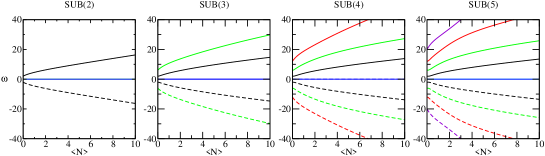
Figure 9: The RPA frequencies for the normal ECCM for $\Omega=10$ at various levels of truncation

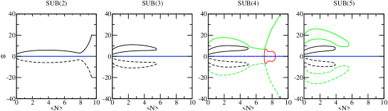
Figure 10: The RPA frequencies for the quasiparticle ECCM for $\Omega=10$ at various levels of truncation

From both these figures, we note that we do see the expected zero modes for excitations breaking particle number, but remaining on the solution branch being studied. These are of course doubly-degenerate. As we increase the level of truncation, more-and-more other modes come in. These also break particle number, as can be seen e.g. at $\langle N\rangle=0$, where the only excited states available are those with different particle number, e.g., the $N=2$ states for SUB(2), $N=2+4$ for SUB(3), etc. The excitations energies are of course also identical for the empty shell for the two schemes, since they coincide at that point. Things change as we move away towards the middle of the shell. Whereas the standard ECCM gives real frequencies, the quasiparticle ECCM solutions meet in pairs (and turn complex), showing a break-down of the approximation scheme. Also, the break-down point seems to move to smaller $N$ as we increase the level of truncation. It also sheds light on the rather different behaviour for even and odd truncation levels seen before: for an even truncation scheme, we always have one odd pair of modes, taking away the pair of zero modes, whereas for an odd truncation level all non-zero modes can and will collide in pairs.

7 Discussion

We have shown that one can formulate a number of CCM based methods for application to problems with pairing. These have been analysed for a rather simple model, and all seem to suffer from some problems. The particle ECCM is the most stable method for low order calculations, but all methods seem to suffer some drawback. The real surprise is that the low order particle ECCM fails as badly as it does–we would have expected it to work best. No detailed understanding of these results exists, but they are clearly linked to the restoration of particle number required in these calculations.

Clearly the exact integrability of the underlying model may also play a role in these results, but one feature will persist: the restoration of the broken particle number means that the exact solutions have zero SUB(1) pairing, suggestive of the fact that different solutions lie on different branches of CCM solutions. This will also lead to instabilities at some order–we do expect that for real system with pairing in large model spaces the problems are much less pronounced, but the comparison of SUB2 NCCM and ECCM seems to be a promising aspect of any approach, as is the study of the particle number fluctuations, which seems to be the best tool to highlight unphysical solutions.

If we were to try and apply an improved many-body method to fermions, e.g., confined in a harmonic trap, any one of the methods discussed here is probably a good choice, as long as we don’t push the order of approximation too high; we must, however, carefully monitor the behaviour of fluctuation in particle number and the local-harmonic modes with ground state symmetry.

References

References

- [1] Coester F and Kümmel H 1960 Nucl. Phys. 17 477 – 485
- [2] Kümmel H, Lührmann K H and Zabolitzky J G 1978 Phys. Rep. 36 1 – 63
- [3] J Čižek 1966 J. Chem. Phys. 45 4256
- [4] J Čižek 1969 Adv. Chem. Phys. 14 35
- [5] Čižek J and Paldus J 1971 Int. J. Quantum Chem. 5 359
- [6] Paldus J, Čižek J and Shavitt I 1972 Phys. Rev. A 5 50
- [7] Bartlett R J and Musial M 2007 Rev. Mod. Phys. 79 291 – 352
- [8] Heisenberg J H and Mihaila B 1999 Phys. Rev. C 59 1440 – 1448
- [9] Mihaila B and Heisenberg J H 1999 Phys. Rev. C 60 054303
- [10] Mihaila B and Heisenberg J H 2000 Phys. Rev. Lett. 84 1403 – 1406
- [11] Mihaila B and Heisenberg J H 2000 Phys. Rev. C 61 054309
- [12] Kowalski K, Dean D J, Hjorth-Jensen M, Papenbrock T and Piecuch P 2004 Phys. Rev. Lett. 92
- [13] Piecuch P, Wloch M, Gour J R, Dean D J, Hjorth-Jensen M and Papenbrock T 2005 Nuclei and mesoscopic physics 777 28 – 45
- [14] Wloch M, Dean D J, Gour J R, Piecuch P, Hjorth-Jensen M, Papenbrock T and Kowalski K 2005 Eur. Phys. J. A 25 485 – 488
- [15] Wloch M, Dean D J, Gour J R, Hjorth-Jensen M, Kowalski K, Papenbrock T and Piecuch P 2005 Phys. Rev. Lett. 94 212501
- [16] Wloch M, Gour J R, Piecuch P, Dean D J, Hjorth-Jensen M and Papenbrock T 2005 J. Phys. G 31 S1291 – S1299
- [17] Dean D J, Hjorth-Jensen M, Kowalski K, Papenbrock T, Wloch M and Piecuch P 2005 Coupled cluster approaches to nuclei, ground states and excited states Key topics in nuclear structure 8th International Spring Seminar on Nuclear Physics ed Covello A (Paestum, Italy) pp 147 – 157
- [18] Dean D J, Gour J R, Hagen G, Hjorth-Jensen M, Kowalski K, Papenbrock T, Piecuch P and Wloch M 2005 Nucl. Phys. B 752 299C – 308C
- [19] Dean D J, Hjorth-Jensen M, Kowalski K, Piecuch P and Wloch M 2006 Condensed matter theories, vol 20 20 89 – 97
- [20] Gour J R, Piecuch P, Hjorth-Jensen M, Wloch M and Dean D J 2006 Phys. Rev. C 74 024310
- [21] Papenbrock T, Dean D J, Gour J R, Hagen G, Hjorth-Jensen M, Piecuch P and Wloch M 2006 Int. J. Mod. Phys. B 20 5338 – 5345
- [22] Hagen G, Papenbrock T, Dean D J, Schwenk A, Nogga A, Wloch M and Piecuch P 2007 Phys. Rev. C 76
- [23] Greiner M, Regal C A and Jin D S 2003 Nature 426 537–540
- [24] Emrich K and Zabolitzky J G 1984 Lec. Notes in Phys. 198 271 – 278
- [25] Emrich K and Zabolitzky J G 1984 Phys. Rev. B 30 2049 – 2069
- [26] Arponen J 1983 Ann. Phys. (NY) 151 311 – 382
- [27] Arponen J S, Bishop R F and Pajanne E 1987 Phys. Rev. A 36 2539 – 2549
- [28] Arponen J S, Bishop R F and Pajanne E 1987 Phys. Rev. A 36 2519 – 2538
- [29] Arponen J, Bishop R F, Pajanne E and Robinson N I 1988 Phys. Rev. A 37 1065 – 1086
- [30] Robinson N I, Bishop R F and Arponen J 1989 Phys. Rev. A 40 4256 – 4276
- [31] Arponen J S and Bishop R F 1990 Phys. Rev. Lett. 64 111 – 114
- [32] Bishop R F and Arponen J S 1990 Int. J. Q. Chem. 197 – 211
- [33] Brueckner K and Wada V 1956 Phys. Rev. 103 1008
- [34] Sekino H and Bartlett R 1984 Int. J. Quantum Chem. Quantum Chem. Symp. 18 255
- [35] Ring P and Schuck P 1980 The Nuclear Many-Body Problem (Springer-Verlag, New York)
- [36] Klein A and Marshalek E 1991 Rev. Mod. Phys. 63, 375 – 558
- [37] Balian R and Brezin E 1969 Nuovo Cim. B 64 37