PostScript file created: ; time 685 minutes
RANDOM STRESS AND OMORI’S LAW
Yan Y. Kagan
Department of Earth and Space Sciences, University of California,
Los Angeles, California 90095-1567, USA;
Emails: ykagan@ucla.edu, kagan@moho.ess.ucla.edu
Abstract. We consider two statistical regularities that were used to explain Omori’s law of the aftershock rate decay: the Lévy and Inverse Gaussian (IGD) distributions. These distributions are thought to describe stress behavior influenced by various random factors: post-earthquake stress time history is described by a Brownian motion. Both distributions decay to zero for time intervals close to zero. But this feature contradicts the high immediate aftershock level according to Omori’s law. We propose that these statistical distributions are influenced by the power-law stress distribution near the earthquake focal zone and we derive new distributions as a mixture of power-law stress with the exponent and Lévy as well as IGD distributions. Such new distributions describe the resulting inter-earthquake time intervals and closely resemble Omori’s law. The new Lévy distribution has a pure power-law form with the exponent and the mixed IGD has two exponents: the same as Lévy for small time intervals and for longer times. For even longer time intervals this power-law behavior should be replaced by a uniform seismicity rate corresponding to the long-term tectonic deformation. We compute these background rates using our former analysis of earthquake size distribution and its connection to plate tectonics. We analyze several earthquake catalogs to confirm and illustrate our theoretical results. Finally, we discuss how the parameters of random stress dynamics can be determined through a more detailed statistical analysis of earthquake occurrence or by new laboratory experiments.
Short running title: Random stress and Omori’s law
Key words: Omori’s law; Random stress; Aftershocks; Lévy distribution; Inverse Gaussian distribution; Seismicity as result of plate-tectonic deformation; Selection bias.
1 Introduction
Our aim is to investigate the connection between random stress and the Omori law of aftershock occurrence. Several attempts to explain Omori’s law have been published. Since stress in the Earth’s interiors cannot be easily measured or calculated, these studies usually consider stress as a scalar stochastic variable, ignoring for a while its tensorial nature. In this work we consider the stress as a scalar.
Here we use the scalar seismic moment directly, but for easy comparison we convert it into an approximate moment magnitude using the relationship
| (1) |
(Hanks, 1992), where is measured in Newton m (Nm). Since we are using almost exclusively the moment magnitude, later we omit the subscript in .
Kagan (1982) considered stress time history as a Brownian motion, i.e., randomly fluctuating stress acting on the stressed environment of an earthquake focal zone. Here the probability density for the time intervals between earthquake events has a Lévy distribution with a power-law tail having the exponent . Kagan and Knopoff (1987) added a tectonic drift component to the Brownian motion. For such a case, the distribution of inter-event times is the Inverse Gaussian distribution (IGD) which, depending on the value of the initial stress drop and velocity of tectonic motion, can exhibit occurrence patterns ranging from the Lévy distribution to a quasi-periodic occurrence.
Matthews et al. (2002) also proposed the IGD as a law for inter-earthquake intervals; however, they considered only a limiting, quasi-periodic long-term distribution. The authors suggest that “… [the Inverse Gaussian] distribution has the following noteworthy properties: (1) the probability of immediate [large earthquake] rerupture is zero; (2) the hazard rate increases steadily from zero at to a finite maximum near the mean recurrence time …” and real earthquake occurrence follows the same pattern. Ellsworth (1995), Ellsworth et al. (1999), Nadeau et al. (1995), and Nadeau and Johnson (1998) present several sequences of recurrent quasi-periodic earthquakes which, in their opinion, confirm a smaller coefficient of variation than the Poisson process for earthquake recurrence intervals.
There is ample evidence that after almost any earthquake subsequent events follow Omori’s law. This has been observed for smaller earthquakes (aftershocks) as well as large events comparable in size to the original shock or even exceeding it (Kagan and Jackson, 1999). Omori’s law pattern of power-law rate decaying seismicity is observed at decadal and centuries long scales (Utsu et al., 1995; Stein and Liu, 2009; Ebel, 2009).
Moreover, the presumed pattern of earthquake quasi-periodicity depends on the argument that stress drops to zero or close to zero in the focal zone of an earthquake. Thus, it would be necessary to wait for some time before a critical stress level is reached. Kagan and Jackson (1999) presented several examples of large earthquakes which followed after a short time interval (often just a few days) within a focal zone of similar large events. Such an inter-earthquake interval is clearly insufficient for stress to be replenished by tectonic motion. We present additional evidence for this pattern later in this paper.
Thus, for relatively short time intervals, earthquakes are clustered in time with the coefficient of variation significantly greater than that for the Poisson process (Kagan and Jackson, 1991). Why is it widely believed that large earthquakes are quasi-periodic in time? Evidence mostly comes from specifically selected sequences (Bakun and Lindh, 1985; Ellsworth, 1995) or from paleo-seismic investigations (Ellsworth et al., 1999). However, paleo-seismic investigations have poor time resolution: two or more events occurring closely in time are likely to be identified as one event. Hence, their coefficient of variation estimates should be biased towards smaller values: a more periodic pattern. Some paleo-seismic investigations (Marco et al., 1996. Rockwell et al., 2000; Ken-Tor et al., 2001; Dawson et al., 2003) also suggest that earthquakes follow a long-term clustering pattern at least in regions of slow tectonic deformation.
Additionally, paleo-seismicity studies the Earth’s displacement only at the surface. But temporal and spatial distributions of earthquakes rupturing the surface at one site substantially differ from general earthquake statistics (Kagan, 2005). The earthquake size distribution is also significantly different for site- and area-based statistics. Rigorously reliable statistical properties that are relevant for theoretical studies as well as for seismic hazard estimates can only be obtained by analyzing instrumental earthquake catalogs.
Measurements from instrumental earthquake catalogs indicate that short time intervals between large earthquakes are much more frequent than even the Poisson model would suggest (Kagan and Jackson, 1991; 1999). Moreover, the problem of biased selection is also hard to avoid in historical and paleo-seismic data: sequences not displaying suggested patterns or with a small number of events are less likely to be considered.
Recently, repeating microquakes have been studied in the Parkfield area (Nadeau et al., 1995; Nadeau and Johnson, 1998, and references therein). These event sequences exhibit certain properties of characteristic quasi-periodic earthquakes: regularity of occurrence and nearly identical waveforms. They show many other interesting features of earthquake occurrence. However, these micro-events are not characteristic earthquakes in a strict sense: they do not release almost all the tectonic deformation on a fault segment while real characteristic earthquakes are assumed to do so.
As with large characteristic earthquakes, attempts using micro-earthquake quasi-periodicity for their prediction have not yet succeeded. Zechar, J. D. (private communication, 2010) attempted to forecast repeating small earthquakes on the San Andreas fault near Parkfield, based on event regularity. While retrospective tests indicated that the forecasts based on recurrence times were better than random, the forward tests were unsuccessful.
Moreover, these micro-events apparently occur on isolated asperities surrounded by creeping zones. Therefore, such an asperity exists as a secluded entity and may produce characteristic quasi-periodic rupture events, similar to fracture in many laboratory experiments. But tectonic earthquakes occur in an environment that is never isolated. This may explain their ubiquitous clustering in time and space.
The quasi-periodic model for characteristic earthquakes (see for example, McCann et al., 1979; Bakun and Lindh, 1985; Nishenko, 1991) has been put to a prospective test using new data. Testing the validity of this hypothesis ended in failure (Rong et al., 2003 and references therein; Bakun et al., 2005; Jackson and Kagan, 2006).
How can we investigate earthquake occurrence patterns in various tectonic zones? Our statistical studies of seismicity (see for example, Kagan, 1991, 2007; Kagan and Jackson, 1991; Kagan et al., 2010) are biased because earthquake rate is dominated by places with a high tectonic rate. Thus, the likelihood function maximum is mainly determined by these earthquakes. However, we should study earthquake patterns in continental areas (active and non-active) where the earthquake rate is low, but the vulnerable human population is large (see Stein and Liu, 2009; Parsons, 2009). A naive extrapolation of aftershock sequence rates would exaggerate seismic hazard. Instead, we need a convincing tool to produce a truer estimate.
Our recent results suggest that earthquake occurrence can be modeled by the Poisson cluster process: the combination of the long-term rate caused by tectonic strain with short-term clustering. For large and medium strain rates, the model appears to work well (see again Kagan et al., 2010). The model is producing reasonable long- and short-term forecasts of earthquake occurrence both for local (Helmstetter et al., 2006) and global (Kagan and Jackson, 2010) seismicity. But to extrapolate such a model to small tectonic rates we would need additional arguments; we must extract the rates by comparing seismicity patterns with tectonic strain maps. Bird et al. (2010) discuss the dependence of the long-term inter-earthquake rate on strain. We need to show how the short-term properties of earthquakes behave in the regions of varying strain. As shown below, the transition time from Omori’s law decay to a quasi-stationary rate clearly increases with a decrease in the strain rate. As the result of these studies, we propose that the same statistical model can be applied for regions of both high and low tectonic strain.
2 Aftershock temporal distribution, theoretical analysis
2.1 Lévy distribution
Kagan (1982) proposed a heuristical model for an earthquake fracture as follows. At the moment that any given earthquake rupture stops, the stress near the edge of the rupture is lower than the critical breaking stress for extension of the fracture. The subsequent stress history near the earthquake rupture tip depends on other fractures in the neighborhood and additional random factors. In this case, the time history of the stress might resemble a Brownian random walk. The stress-time function is thus given as a solution to the diffusion equation. When the stress reaches a critical threshold level, a new earthquake begins. The distribution density of the time intervals of the ‘first passage’ (Feller, 1966) is the Lévy distribution
| (2) |
where is the diffusion coefficient, is the time, and is the threshold or barrier stress: the difference between initial breaking stress and that when rupture ceases. This distribution as a function of stress is the Rayleigh law; as a function of time it is the Lévy distribution (cf. Zolotarev, 1986). In this model, the stress is taken to be a scalar, which corresponds to the addition of perfectly aligned stress tensors; the interaction of misaligned tensors will be discussed in a later work. The Lévy distribution (1) was used by Kagan (1982, see Eqs. 8 and 9) to model the time dependent part of the space-time sequence of micro-earthquakes. Here we are address only the time sequence of events.
Fig. 1 displays several Lévy curves for various values of stress drop, . The curve’s tail is a power-law similar to that exhibited by Omori’s law. However, for small values of time the curves decay to zero: depending on the stress drop, Brownian motion takes time to reach a critical stress level. This latter feature, though observed in aftershock sequences, is most likely caused by effects from coda waves of both the mainshock and stronger aftershocks that prevent identifying smaller aftershocks (Kagan, 2004). This opinion is supported by aftershock registration in the high-frequency domain (Enescu et al., 2009) where their time delay is substantially reduced. Measurements of total seismic moment rate decay in aftershock sequences (Kagan and Houston, 2005) suggest that aftershocks start right after the end (within one minute for a earthquake) of a mainshock rupture. Therefore, the left-hand decay of the curves in Fig. 1 is not realistic.
There is another problem in comparison of theoretical distribution with aftershock observations. The Lévy curves may explain the inter-event time statistics only for the first generation (parent-child) of clustered earthquakes. Most observed aftershocks or clustered events are generally separated from their ‘parents’ by multiple generations. For example, the present aftershocks of the 1811-12 New Madrid earthquakes or the 1952 Kern County, California, earthquake are mostly distant relatives of their progenitors (mainshocks). In the Omori law we count all aftershocks, disregarding their parentage, whereas the Lévy law describes the time distribution for the next event: when the stress level reaches a critical value to trigger a new rupture. When we count all events, we decrease the exponent from 1.5 to 1.0 (Kagan and Knopoff, 1987).
We assume that the next earthquake may occur in any place in the focal zone of a previous event. Attempts to localize the initiation of strong earthquakes have not been successful; for example, the 2004 Parkfield earthquake occurred well outside the previously specified area (Jackson and Kagan, 2006).
We also assume that the stress drop after an earthquake has a power-law distribution: it is proportional to , for . Kagan (1994), Marsan (2005), Helmstetter et al. (2005), Lavallée (2008), Powers and Jordan (2010) support this statement.
Then for the Lévy distribution we obtain
| (3) |
where is a gamma function. The new modified Lévy distribution density function is a power-law with the exponent . The density should be truncated at the left side, because aftershocks cannot be observed at short-time intervals close to a mainshock (Kagan, 2004). Normalizing the distribution would depend on this truncation. Kagan (1991, Eq. 8) introduced a minimum time (), where is a seismic moment of a preceding event (see also Eq. 17 below). Before that time, the aftershock rate is measured with a substantial undercount bias (Kagan, 2004).
2.2 Inverse Gaussian distribution
As Matthews et al. (2002) indicate, the Inverse Gaussian Distribution (IGD) has been known since 1915. However, this distribution only acquired its name in 1945. This is the name found in recent statistical encyclopedias and books (for example, Kotz et al., 2006; Seshadri, 1999; Chhikara and Folks, 1989), on the Wolfram website, and in Wikipedia, while the “Brownian passage-time” (BPT) is little known. Kagan and Knopoff (1987) proposed to use this distribution (without calling it IGD) to describe the inter-earthquake time distribution. Their major impetus was to explain aftershock statistics (Omori’s law) by stress dynamics.
Here we discuss the appropriate pairwise interval law for a model in which a steadily increasing source of stress, which we take to be due to plate tectonics, is added to or subtracted from a random or diffusion component, where the distribution (2) describes the density of earthquake recurrence times in the absence of tectonic loading. If the rate of tectonic loading is a constant V, the distribution density is modified to (Feller, 1966, p. 368) become the Inverse Gaussian distribution
| (4) |
For tectonic loading velocity , this equation transforms to (2). Fig. 2 displays several IGD curves for various values of stress drop. For small values of and , the curves are similar to the values of Lévy distribution (2): if the stress drop is insignificant, or the tectonic loading influence is small in initial stages of stress behavior.
Assuming again that the stress in a fault neighborhood is distributed according to a power-law, we obtain a new modified distribution of inter-earthquake time, based on the IGD (4)
| (5) | |||||
where is a Kummer confluent hypergeometric function (Wolfram, 1999; Abramowitz and Stegun, 1972, p. 504). Another expression for the density is
| (6) |
where a confluent hypergeometric function (ibid.). As in Eq. 3, both of the above distributions should be truncated as and can be normalized after it.
For certain values of the expressions (5 and 6) can be simplified. For example for
| (7) |
For we obtain two equations. For a positive , using Eq. 13.6.3 by Abramowitz and Stegun (1972), we transform (5) into
| (8) |
where and are modified Bessel functions (Wolfram, 1999; Abramowitz and Stegun, 1972, p. 374).
For a negative using Eq. 13.6.21 by Abramowitz and Stegun (1972), we transform (6) into
| (9) |
where is a modified Bessel function (Wolfram, 1999; Abramowitz and Stegun, 1972).
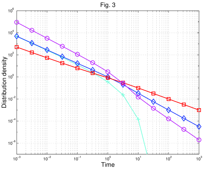
In Fig. 3 we display the new IGD curves for various values of the parameter. Although the general behavior of the curves remains power-law, the curves change their slope at the time value of about 1.0. The curves with show the distribution difference for tectonic loading sign; in the positive case tectonic movement is opposite to the fault displacement during an earthquake, whereas the negative sign corresponds to motion consistent with the earthquake mechanism. In the latter case, random fluctuations can bring the fault to rupture only during the early period of development.
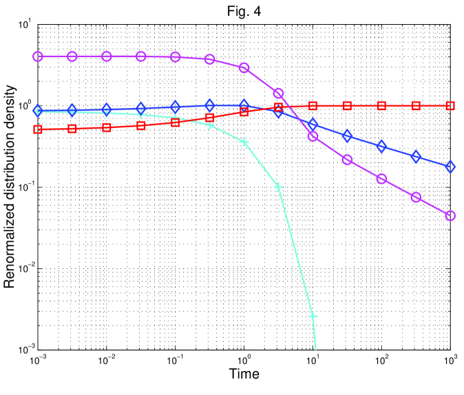
To show the curves’ behavior more clearly in Fig. 4, the PDF values are multiplied by . For small time intervals curves are horizontal, suggesting that the modified IGD is similar to the Lévy distribution in Eq. 3.
For small time values, the power-law exponents in Fig. 3 are essentially the same as for compounded Lévy law (3). This can be seen from modified Bessel function approximations for small values of the argument (Abramowitz and Stegun, 1972, Eqs. 9.6.7 and 9.6.9),
| (10) |
In the general case the same result can be obtained with Eq. 13.5.5 by Abramowitz and Stegun (1972). Then for Eq. 5 transforms into
| (11) |
It is obvious from Figs. 3 and 4 that, except for the curve, the slope of curves for large values of the time increases when compared with close to zero. Using Eq. 13.1.27 of Abramowitz and Stegun (1972) we add an exponential term in (5) within the hypergeometric function . Then for we obtain
| (12) |
(Abramowitz and Stegun, 1972, Eq. 13.5.1). Therefore, in Eq. 8 the exponent would be (Abramowitz and Stegun, 1972, Eq. 9.7.1), whereas in Eq. 9 the power-law term (Abramowitz and Stegun, 1972, Eq. 9.7.2) is multiplied by an exponential decay term
| (13) |
3 Temporal distribution of aftershocks: Observations
Many observations of Omori’s law behavior have been published (see Utsu et al., 1995 and references therein). There are some problems with these measurements. The standard interpretation of the Omori law is that all aftershocks are caused by a single mainshock. However, the mainshock is often followed by strong aftershocks and those are clearly accompanied by their own sequence of events, and so on. The second problem is that some earthquakes have very few or no aftershocks; such sequences cannot be included in the naive study of earthquake sequences, but can be analyzed as stochastic processes.
Thus, three techniques can be applied to study the temporal distribution of real earthquakes: 1) traditional, phenomenological techniques based on observing individual aftershock sequences; 2) using statistical moments of earthquake occurrence, considered as a point process; 3) applying stochastic process modeling to infer the parameter values of earthquake temporal interaction.
3.1 Aftershock sequences
Beginning with Omori (1894), the temporal distribution of aftershock numbers has been studied for more than one hundred years (Utsu et al., 1995). Aftershock rate decay is approximated as with parameter value close to 1.0 (Kagan, 2004).
But the simple, superficial study of aftershock rate decay often encounters serious problems. First, only relatively rich aftershock sequences can be investigated by direct measurements; if there are too few aftershocks, their properties can be studied only by combining (stacking) many sequences. Second, to isolate individual sequences one should exclude any cases when one sequence is influenced by another, an arbitrary procedure which may introduce a selection bias. Third, an aftershock sequence often contains one or several large events which are clearly accompanied by a secondary aftershock sequence. Taking the influence of secondary earthquakes into account is not simple (see Section 3.3 for more detail). Fourth, some sequences start with a strong foreshock which is sometimes only slightly weaker than a mainshock. Again, handling this occurrence presents serious problem.
Therefore, strong bias may result from directly measuring Omori’s law exponents. Two other statistical methods considered below enable analysis of the whole earthquake occurrence as a point process, to minimize the problem of data and interpretation technique selection bias.
3.2 Temporal distribution for earthquake pairs
Kagan and Jackson (1991) investigated space-time pairwise earthquake correlation patterns in several earthquake catalogs. They showed that earthquake pairs follow a power-law distribution for small time and distance intervals. Kagan and Jackson (1999) showed that contrary to the seismic gap model the clustering pattern continues for strong () earthquakes. Large shallow earthquakes can re-occur after a small time interval.
Table 1 shows the location and focal mechanism difference for global shallow earthquakes in the GCMT catalog (Ekström et al., 2005; Ekström, 2007) from 1976-2010. The table format is similar to Table 1 in Kagan and Jackson (1999). However, here we kept only those pairs in the table for which their focal zone overlap (the -parameter) is greater than 1.0:
| (14) |
where and are the respective rupture lengths for the first and second earthquakes in the pair (see Eq. 3 in Kagan and Jackson, 1999) and is the distance between the centroids. Therefore, if the earthquake focal zones would intersect. For several doublets , implying that the smaller event should be largely within the focal zone of the larger earthquake. Inspecting the time difference and the 3-D rotation angle between focal mechanisms suggests that these high pairs may occur after very short time intervals and have very similar double-couple mechanisms.
All earthquakes in the table occur in subduction zones as defined in Kagan et al. (2010). However, even with relatively high deformation velocity at these plate boundaries, the inter-earthquake time is in most cases substantially lower than the time necessary for tectonic motion to restore the critical stress conditions by the occurrence time of the second earthquake (see the last column in Table 1 by Kagan and Jackson, 1999).
Fig. 5 shows how the normalized number of shallow earthquake pairs depends on the tectonic deformation rate as defined by Bird et al. (2010). Three curves are shown: all earthquakes from the GCMT catalog, earthquakes from subduction zones (Kagan et al., 2010), and events from active continental zones.
Fig. 6 shows the integration domain for calculating earthquake pair rates. The diagram is a square with a side length equal to a catalog duration, ; since the plot is symmetric, only the lower-right portion of the square is shown. The first event shown as a filled circle, is supposed to be at the square diagonal, the second one at the end of a hatched area. We assume that the time difference between earthquakes cannot be less than (similar to in Eq. 17).
For the Poisson process, the interval pair density is uniform (see Kagan and Jackson, 1991, Eq. 1). Thus, the rate is proportional to the hatched area. For the normalized survival rate
| (15) |
where is the minimum time interval, is the catalog duration and is the inter-earthquake time interval.
For the power-law time distribution with distribution density , we obtain the normalized survival rate by integrating over the domain shown in Fig. 6:
| (16) |
In Figs. 7-10 the temporal distribution of inter-earthquake times for event pairs is shown as it depends on earthquake rate determined by Bird et al. (2010). Several approximations for pair intervals are also given: the Poisson distribution of earthquakes (15) in the time span 1976-2010 and a few power-law interval (16) dependencies.
Obviously distribution curves consist of two parts: for small time intervals, they follow a power-law and for larger intervals the distribution is parallel to the Poisson rate. The transition from one behavior to another occurs sooner for zones with a higher tectonic deformation rate: in Fig. 7 the transition is observed for the time of about 6,000 days; in Fig. 8 it is about 4,000-5,000 days, and in Fig. 9 it is less than 3,000 days.
Fig. 10 shows the time interval distribution for active continental areas. In this case a visual inspection suggests that the best approximation is the power-law; no transition to the Poisson rate is observable. This absence can be explained by a low deformation rate in these zones (see Fig. 5). As was observed for many aftershock sequences in continental and slowly deforming areas, aftershock sequences continue according to Omori’s law for decades and even centuries (Utsu et al., 1995; Stein and Liu, 2009; Ebel, 2009). Here the span of 34 years covered by the GCMT catalog is likely insufficient to demonstrate the transition from an aftershock sequence to a background, Poisson rate.
We compute an average recurrence time () for earthquakes in Figs. 7-10. The smallest value for is observed for distributions with a significant component of the power-law: Figs. 7 and 10. We also calculate the coefficient of variation () of earthquake inter-occurrence time as a ratio of the standard deviation () to the average time (Kagan and Jackson, 1991). A completely random Poisson occurrence has the coefficient of variation equal to one, whereas quasi-periodicity yields a coefficient of less than one. It yields the coefficient larger than one for clustered earthquakes. Although the estimates are biased when determined at a relatively short catalog time span, their mutual relations are indicative of occurrence patterns. For Figs. 7-10, the -values are 1.10, 0.925, 0.841, and 1.977, respectively. These evaluations again suggest that earthquakes in areas with a smaller tectonic rate become more clustered, and their Poisson component is diminished.
3.3 Stochastic branching processes
As we mentioned above, the mainshock is often followed by strong aftershocks and those are clearly accompanied by their own sequence of events, and so on. The patterns of multiple clustering have been described by stochastic branching processes (Hawkes and Adamopoulos, 1973; Kagan, 1991; Ogata, 1998). In this model, seismicity is approximated by a Poisson cluster process, in which clusters or sequences of earthquakes are statistically independent, although individual events in the cluster are triggered. However, Brémaud and Massoulié (2001) proposed a model in which all events belong to one branching cluster.
Kagan et al. (2010) applied the Critical Branching Models (CBM) to analyze earthquake occurrences statistically in several global and regional earthquake catalogs. Time intervals between earthquakes within a cluster are assumed to be distributed according to a power-law
| (17) |
This is similar to Omori’s law. The parameter is an ‘earthquake memory’ factor, is the coda duration time of an earthquake with seismic moment , and is the branching (productivity) coefficient (Kagan et al., 2010, Eq. 9).
During a likelihood search the -values have been restricted within the interval ; smaller or larger estimates are inadmissible because of physical considerations (Kagan, 1991; Kagan et al., 2010). Fig. 11 shows a correlation between two parameters and of the CBM. Most -values are within the interval and are negatively correlated with the coefficient.
Several determinations of the time decay exponent are carried out for the ETAS (Epidemic Type Aftershock Sequence) model. Ogata (1998, Tables 2-3) obtained the -values (equivalent to our coefficient), of the order 1.03–1.14. Ogata et al. (2003, Tables 1-2) estimates the -values to vary within 1.05–1.18. Ogata and Zhuang’s (2006, Tables 2-3) values are 1.02–1.05. Zhuang et al. (2005) obtained -values of 1.14–1.15. Helmstetter et al. (2006, Table 1) used a branching model similar to the ETAS and calculated .
To illustrate our fit of the temporal distribution of dependent earthquakes, average numbers of aftershocks following 15 GCMT earthquakes are displayed in Fig. 12 (similar to Fig. 13 in Kagan, 2004). We use the time period 1977-2003, so that all large earthquakes are approximately the same size (, i.e., excluding the 2004 Sumatra and its aftershocks). Since the GCMT catalog has relatively few dependent events, we selected aftershocks from the the U.S. Geological Survey (2010) PDE (Preliminary Determinations of Epicenters) catalog. The aftershock rate in the diagram is approximately constant above our estimate of the coda duration . For the logarithmic intervals, this corresponds to the standard form of the Omori law: the aftershock number is proportional to . For the smaller time intervals, the aftershock numbers decline when compared to the Omori law prediction (). This decline is caused by several factors, the interference of mainshock coda waves being the most influential (Kagan, 2004). The decline is faster for weaker events (ibid.).
For theoretical estimates, we used the values of parameters obtained during the likelihood function search (Kagan et al., 2010, Table 4) obtained for the full PDE catalog, : the branching coefficient , the parent productivity exponent (), and the time decay exponent . Theoretical estimates in Fig. 12 seem to be reasonably good at forecasting time intervals on the order of one day. For larger intervals, the expected numbers decrease as : this is stronger than the regular Omori law would predict. As we suggested in Section 2.1 the Omori law assumes that all aftershocks are direct consequences of a mainshock, whereas a branching model regards any earthquake as a possible progenitor of later events. Thus, later aftershocks are the combined offspring of a mainshock and all consequent earthquakes. With increase in time, the difference between Omori’s law and the CBM predictions would increase as well. Marsan and Lengliné (2008) show that in California catalogs due to cascading aftershock rates for direct and secondary triggering differ by a factor of 10 to about 50%. By numerical simulations of the ETAS model, Felzer et al., (2002) and Helmstetter and Sornette (2003) estimated that a substantial majority of aftershocks are indirectly triggered by the mainshock.
The -parameter in Omori’s law is often assumed to be 1.0. This -value implies that the total aftershock number approaches infinity as the duration of the aftershock sequence increases. Figs. 3 and 4, however, suggest that in the presence of tectonic loading, the time exponent value should increase at longer time periods. Statistical determination of the exponent can usually be made for only short periods; thus, we do not yet have a good estimate of the -value for the tail of an aftershock sequence.
4 Earthquake statistics and plate-tectonic deformation
4.1 Stationary earthquake rate due to tectonic deformation
The tapered Gutenberg-Richter (TGR) relation (Kagan, 2002b) has an exponential taper applied to the number of events with a large seismic moment. Its survivor function ( cumulative distribution) for the scalar seismic moment is
| (18) |
Here is the parameter controlling the distribution in the upper ranges of (‘the corner moment’), is the moment threshold: the smallest moment above which the catalog can be considered to be complete; is the index parameter of the distribution; , is a familiar -value of the Gutenberg-Richter distribution (G-R, Gutenberg and Richter, 1944).
By evaluating the first moment of the distribution (18), we can obtain a theoretical estimate of the seismic moment flux (Kagan, 2002b)
| (19) |
where is a gamma function and is the seismic activity level (occurrence rate) for earthquakes with moment and greater.
We compare the seismic moment rate with the tectonic moment rate ():
| (20) |
where is the seismic coupling (or seismic efficiency) coefficient, is the elastic shear modulus, is the seismogenic width of the lithosphere, is the average horizontal strain rate, and is the area under consideration. At present, some variables in the equation cannot be evaluated with great accuracy; to overcome this difficulty we calculate a product of these variables: the ‘effective width’ of seismogenic zone or coupled seismogenic thickness (Bird and Kagan, 2004):
| (21) |
Bird and Kagan (2004, Eq. 11) propose another, more exact formula for calculating the tectonic moment rate appropriate to a plate boundary zone.
In regions of high seismicity, instead of Eqs. 19–21 we can use measured long-term seismic activity to infer the earthquake rate by extrapolating (18) to any moment level (see Bird and Liu, 2007, Eqs. 4 and 5). Bird et al. (2010) presented an algorithm and tables for a long-term world-wide forecast of shallow seismicity based on the Global Strain Rate Map (GSRM) by Kreemer et al. (2003). Because GSRM does not estimate tectonic strain-rates of stable plate interiors, a simple empirical-averaging method has been used. Thus, the seismicity in plate interiors is represented by a uniform rate.
Since the seismicity level in plate interiors may vary by orders of magnitude, the uniform rate may strongly under- or over-estimate the seismicity rate. Therefore, we apply Eqs. 19–21 to evaluate first the tectonic moment rate and then a long-term forecast for these regions
| (22) |
By calculating for a particular choice of , we may re-normalize Eq. 18 and obtain earthquake size distribution for any region with a known strain rate and corner moment.
4.2 Length of aftershock zone
Eq. 22 above can be used to evaluate the background seismicity level for an aftershock zone. Such a calculation would use the area of an earthquake focal zone. This area can be estimated by a dimension of aftershock zone for each event. Kagan (2002a) evaluated how the aftershock zone size for mainshocks depends upon on the earthquake magnitude by approximating aftershock epicenter maps through a two-dimensional Gaussian distribution. The major ellipse axis is taken as a quantitative measure of the mainshock focal zone size.
In Fig. 13 we display the regression curves for GCMT/PDE earthquakes: all earthquakes for three choices of focal mechanisms (updated Fig. 6a by Kagan, 2002a). In regression curves we use as a reference point. For example, for the quadratic regression
| (23) |
where is the length of the aftershock zone in km. For the linear regression we set . Fig. 14 displays the regression in a similar format for active continental tectonic zones (Kagan et al., 2010).
Table 2 summarizes the results of regression analysis for all global earthquakes, as well as for events in subduction zones (trenches) and on active continental zones. Earthquakes are also subdivided by their focal mechanism. Other tectonic zones lack a sufficient number of mainshocks to carry out this statistical analysis.
The following conclusions can be made from Table 2: (a) aftershock zones exhibit similar scaling; (b) zone length () on average is proportional to moment ; and (c) the value of parameter (zone length for the earthquake) is close to (316) km for all cases. Normal earthquakes (rows 5-6) exhibit slightly different scaling; zone length () for the linear regression is proportional to moment . Scaling for strike-slip earthquakes (rows 7-8) also differs a little from average: zone length () is proportional to moment . However, the earthquake numbers in these subsets are small, thus it is possible that these variations are due to random fluctuations.
Only three subsets show a substantial nonlinearity: (a) trenches with strike-slip focal mechanisms (rows 15-16); (b) continents with all focal mechanisms (rows 17-18); and (c) continents with strike-slip focal mechanisms (rows 21-22). However, the earthquake numbers are small in all these plots, and although (b) and (c) aftershocks display zone lengths which increase strongly for the largest earthquakes (the feature often quoted in other studies of length scaling – see, for instance, Wells, and Coppersmith, 1994, and subsequent publications citing that paper), (a) earthquakes exhibit an opposite behavior.
In all diagrams the standard errors () are almost the same for the linear and quadratic regression. The maximum errors () follow the same pattern. This pattern suggest that linear regression is sufficient to approximate the data. Although the quadratic regression fit yields no statistically significant improvement in almost any diagram, the sign of the quadratic correction term is negative for most cases. The negative value of the regression coefficient means that increase in the aftershock zone length is weaker for the largest earthquakes. This feature contradicts those often quoted in other studies of length scaling (see Kagan, 2002a for details). Thus, the slope of the regression curve is either stable or decreases at the high magnitude end. No saturation effect for large earthquakes occurs in the data. Results in Table 2 imply that the major ellipse axis (length) of an earthquake focal zone can be approximated by
| (24) |
We conclude that earthquake rupture length is proportional to the cube root of moment, which implies that width and slip should scale the same way. Otherwise, one of them increases less strongly with moment and the other more strongly. For either that would pose the problem of “inverse saturation.”
We assume that the majority of aftershocks are concentrated within an ellipse having 2- major axis. The probability that a point lies inside a 2- ellipse is shown in Eq. 5 by Kagan (2002a). If we know the length of an earthquake focal zone, we can calculate its area. We assume, for example, that the ratio of the major ellipse axis to the minor axis is 1/4; then area of the focal zone is
| (25) |
4.3 Example: New Madrid earthquake sequence of 1811-12
To illustrate the arguments and results of the previous sections, we calculate seismicity parameters of the New Madrid earthquake sequence (1811-12) and its consequences. There is substantial literature on this sequence (Stein and Liu, 2009; Calais et al., 2010, and references therein).
Three or four large earthquakes with magnitudes on the order of 7.5–8.0 occurred over a few months of 1811-12 in the New Madrid area; aftershocks of these events are still registered. As an illustration, we would assume that only one event occurred at that time. If in reality earthquakes were smaller than such an event, their total focal zone and combined aftershock sequence at the present time would be equivalent to about one mainshock.
The size of the focal zone can be evaluated by using regression equations in Figs. 13 and 14. The first plot contains many earthquakes but most of these events are in subduction zones. The second diagram uses earthquakes in active continental zones; a focal size of these earthquakes is likely to resemble the New Madrid area which can be classified as plate-interior (Kagan et al., 2010). Too few large earthquakes are available within plate-interior to obtain their features. The difference between regression parameters in Figs. 13 and 14 is small; therefore the size of earthquake focal zones either does not change in various tectonic zones or changes slightly.
For an earthquake, calculations yield 227 km and 259 km as the length of the focal zone, defined as the major axis of an ellipse comprising a majority of aftershocks (Kagan, 2002a). The linear regression is used in both cases: the former value corresponds to Fig. 13 and the latter to Fig. 14. The two estimates are similar and roughly correspond to the size of the present aftershock zone, as shown, for example, in Calais et al. (2010).
To calculate the surface area of an aftershock zone, we assume that the minor axis of the ellipse is 1/4 of the major axis, taken as 240 km. Then we obtain the earthquake focal area as 11300 km2. Taking the average strain rate as (Calais et al., 2006), we compute the tectonic moment rate (20): Nm/year. Assuming that 50% of the tectonic rate is released seismically (Bird and Kagan, 2004), we obtain the background rate earthquakes per year [we take in (22) Nm, km, ; then ]. We use (18) to calculate the recurrence time for an earthquake in the focal zone of the New Madrid events: more than two million years. In this computation any earthquake with an epicenter or centroid in the focal zone counts: in Eq. (22) we do not request that the entire rupture of such an earthquake be contained in the zone. The recurrence time is an average value; even for events as large as the earthquake occurrence is clustered (see Section 3.2). Thus, a new large earthquake can follow after a relatively short time period, as exemplified by the 1811-12 New Madrid sequence.
We would like to calculate the duration of an aftershock sequence up until the aftershock rate decays to the background level. The results in Fig. 12 can be applied to this purpose. However, we need to make a correction for the mainshock and aftershock magnitudes ( instead of and instead of in the plot, respectively). In the diagram the aftershock rate per one interval (the intervals increase consequently by a factor of two) is 7 events. This translates into 4.55 events per interval for our choice of magnitudes (Kagan at al., 2010). After comparing the background and aftershock rates (we take 4.55 aftershocks per the first day, decaying according to Omori’s law, with rate with time), we discover that the aftershock sequence would reach the background rate in about 3,600 years. This duration estimate agree roughly with Stein and Liu’s (2009) value. In these calculations, we presume that no independent large earthquake clusters would occur during the aftershock sequence. The possible occurrence of spontaneous events makes any evaluation of aftershock sequence duration largely approximate.
Stein and Liu (2009) obtained aftershock duration values for several sequences using Eq. 14 from Dieterich (1994). This equation employs parameters whose values for actual earthquake focal zones are not known. Generally, the parameters have been back adjusted based on the statistics of earthquake occurrence. This may explain apparently reasonable fit of Dieterich’s formula to aftershock sequences.
In contrast, we obtain the aftershock sequence duration by extending the tapered Gutenberg-Richter and Omori’s laws and using their well-known properties and measured geometrical features of tectonic deformation. Moreover, according to Stein and Liu (2009, Fig. 1c) the New Madrid aftershock rate for the last 50 years was about 0.5 events per year. Computations based on Omori’s law similar to those shown above, yield the rate 175 years after the mainshock occurrence of about events per year. This number is close to that shown above.
5 Discussion
Two classical statistical earthquake distributions largely governed our approach to analyzing seismicity: Omori’s law and the Gutenberg-Richter relation. As explained above, recent developments in earthquake size statistics considerably improved our understanding of earthquake occurrence and could lead to significantly better estimates of seismic hazard. For the G-R law the earthquake temporal distribution is mostly irrelevant, since size distribution of clustered events is largely independent of their history. Similar progress in understanding earthquake time statistics is much more difficult to achieve. We cannot ignore spatial variables and the available data are not as extensive, so the task is more complex. Only by applying rigorous methods, by analyzing carefully systematic and random effects, and by critical testing of models and hypotheses we will be able to advance in solving this problem.
In previous sections we derived the time distribution for earthquake occurrence; the distribution is shown to be controlled by power-laws. How can the parameters of these distributions be determined? If one excludes the interiors of plates, the tectonic deformation rate is reasonably well known for plate boundaries and for active continents (Kagan et al., 2010; Bird et al., 2010). The diffusion rate is presently unknown. If we could obtain the earthquake temporal distribution as shown in Figs. 1 and 2, the evaluation would be easy. These distributions are derived for a particular area within an earthquake fault zone. However, if the stress in the focal zone of an earthquake is distributed according to the power-law with an exponent (see Eqs. 3 and 5), the problem becomes more acute.
Figs. 3 and 4 suggest that the distribution temporal behavior changes when . This change relates to the first generation of offspring. Thus, we should not be able to see it in regular Omori plots which combine many generations of aftershocks. The inversion of earthquake occurrence parameters based on stochastic branching processes yields needed first generation effects. However, in present models (both CBM and ETAS) as discussed in Section 3.3, temporal dependence is parameterized by just one exponent. These models should in principle demonstrate changes in the temporal pattern, if more complicated temporal function is applied. However, results from statistical analysis are very uncertain even for one-parameter time decay. Given the contemporary quantity and quality of earthquake catalogs, it is unlikely more complicated models would be effective in resolving this issue.
Perhaps new laboratory experiments (Zaiser, 2006) may help solve the problem of diffusion rate evaluation, but it is not clear whether such measurements are possible. The acoustic emission event rate exhibits fore- and aftershock sequences associated with dynamic failure of the test specimen (see, for example, Ojala et al., 2004). These and similar tests can be used to infer the dependence of the Omori law parameters on spatial scale and stress diffusion rate.
Results from statistical analysis of earthquake occurrence in our previous publications (Kagan, 2002b; Bird and Kagan, 2004; Kagan et al., 2010), as well as the results reported above, suggest that the earthquake process in all tectonic provinces can be described by the same model. We advocate the Poisson cluster process with clusters controlled by a critical branching process and a power-law time dependence. Combined with the earthquake size distribution approximation by the TGR, such a model allows mathematically forecast of a spatially variable, time-independent (long-term) earthquake rate. It will optimally smooth the seismicity record (Kagan and Jackson, 2010) or translate the plate-tectonic and geodetic rate into a seismic hazard estimate (Bird and Liu, 2007; Bird et al., 2010).
A short-term forecast can be performed by using the temporal properties of earthquake clusters, an extrapolation which uses a variant of Omori’s law to estimate future earthquake rate (Kagan and Jackson, 2010). In Section 4.3 we presented an example of such calculations.
In conclusion, this paper suggests a method for calculating long- and short-term seismicity estimates, based on theoretical inference about classical, statistical earthquake distributions: the Omori law and the G-R relation. Statistical analysis of earthquake occurrence carried out in our previous papers and in this work make such seismic hazard evaluation more reliable and accurate.
Acknowledgments
I am grateful to Dave Jackson, Paul Davis, and Peter Bird for useful discussion and suggestions. Per Jögi helped with the mathematica computations. I thank Kathleen Jackson for significant improvements in the text. The author appreciates support from the National Science Foundation through grant EAR-0711515, as well as from the Southern California Earthquake Center (SCEC). SCEC is funded by NSF Cooperative Agreement EAR-0529922 and USGS Cooperative Agreement 07HQAG0008. Publication 0000, SCEC.
References
Abramowitz, M. and Stegun, I. A., (Eds.), 1972. Handbook of Mathematical Functions, Dover, NY, pp. 1046.
Bakun, W. H., and A. G. Lindh, 1985. The Parkfield, California, earthquake prediction experiment, Science, 229, 619-624.
Bakun, W. H., B. Aagaard, B. Dost, W. L. Ellsworth, J. L. Hardebeck, R. A. Harris, C. Ji, M. J. S. Johnston, J. Langbein, J. J. Lienkaemper, A. J. Michael, J. R. Murray, R. M. Nadeau, P. A. Reasenberg, M. S. Reichle, E. A. Roeloffs, A. Shakal, R. W. Simpson, and F. Waldhauser, 2005. Implications for prediction and hazard assessment from the 2004 Parkfield earthquake, Nature, 437, 969-974.
Bird, P., and Y. Y. Kagan, 2004. Plate-tectonic analysis of shallow seismicity: apparent boundary width, beta, corner magnitude, coupled lithosphere thickness, and coupling in seven tectonic settings, Bull. Seismol. Soc. Amer., 94(6), 2380-2399 (plus electronic supplement).
Bird, P., C. Kreemer, and W. E. Holt, 2010. A long-term forecast of shallow seismicity based on the Global Strain Rate Map, Seismol. Res. Lett., 81(2), 184-194 (plus electronic supplement).
Bird, P., and Z. Liu, 2007. Seismic hazard inferred from tectonics: California, Seism. Res. Lett., 78(1), 37-48.
Brémaud, P., and L. Massoulié, 2001. Hawkes branching point processes without ancestors, J. Applied Probability, 38(1), 122-135.
Calais, E., Han, J. Y., DeMets, C., Nocquet, J. M., 2006. Deformation of the North American plate interior from a decade of continuous GPS measurements, J. Geophys. Res., 111(B6), B06402, doi:10.1029/2005JB004253.
Calais, E., Freed, A. M., Van Arsdale, R. & Stein, S. (2010). Triggering of New Madrid seismicity by late-Pleistocene erosion, Nature, 466, 608-611
Chhikara, R., and J. L. Folks, 1989. The Inverse Gaussian Distribution, New York, M. Dekker, 213 pp.
Dawson, T. E., S. F. McGill, and T. K. Rockwell (2003), Irregular recurrence of paleoearthquakes along the central Garlock fault near El Paso Peaks, California, J. Geophys. Res., 108(B7), 2356, doi:10.1029/2001JB001744.
Dieterich, J., 1994. A constitutive law for rate of earthquake production and its application to earthquake clustering, J. Geophys. Res., 99, 2601-2618.
Ebel, J. E., 2009. Analysis of aftershock and foreshock activity in stable continental regions: implications for aftershock forecasting and the hazard of strong earthquakes, Seismological Research Letters, 80(6), 1062-1068.
Ekström, G., 2007. Global seismicity: results from systematic waveform analyses, 1976-2005, in Treatise on Geophysics, 4(4.16), ed. H. Kanamori, pp. 473-481.
Ekström, G., A. M. Dziewonski, N. N. Maternovskaya and M. Nettles, 2005. Global seismicity of 2003: Centroid-moment-tensor solutions for 1087 earthquakes, Phys. Earth planet. Inter., 148(2-4), 327-351.
Ellsworth, W. L. (1995). Characteristic earthquakes and long-term earthquake forecasts: implications of central California seismicity, in F. Y. Cheng and M. S. Sheu (Editors), Urban Disaster Mitigation: The Role of Science and Technology, Elsevier Science Ltd., Oxford.
Ellsworth, W. L., M. V. Matthews, R. M. Nadeau, S. P. Nishenko, P. A. Reasenberg, and R. W. Simpson (1999). A physically based earthquake recurrence model for estimation of long-term earthquake probabilities, U.S. Geol. Surv. Open-File Rept. 99-522.
Enescu, B., J. Mori, M. Miyazawa, and Y. Kano, 2009. Omori-Utsu law -values associated with recent moderate earthquakes in Japan, Bull. Seismol. Soc. Amer., 99(2A), 884-891.
Feller, W., 1966. An Introduction to Probability Theory and its Applications, 2, J. Wiley, New York, 626 pp.
Felzer, K. R., T. W. Becker, R. E. Abercrombie, G. Ekström and J. R. Rice, 2002. Triggering of the 1999 7.1 Hector Mine earthquake by aftershocks of the 1992 7.3 Landers earthquake, J. Geophys. Res., 107(B9), 2190, doi:10.1029/2001JB000911.
Gutenberg, B. and Richter, C.F., 1944. Frequency of earthquakes in California, Bull. seism. Soc. Am., 34, 185-188.
Hanks, T.C., 1992. Small earthquakes, tectonic forces, Science, 256, 1430-1432.
Hawkes, A. G., and L. Adamopoulos, 1973. Cluster models for earthquakes - Regional comparisons, Bull. Int. Statist. Inst., 45(3), 454-461.
Helmstetter, A., and D. Sornette, 2003. Importance of direct and indirect triggered seismicity in the ETAS model of seismicity, Geophys. Res. Lett., 30(11), 1576, doi:10.1029/2003GL017670.
Helmstetter, A., Y. Y. Kagan, and D. D. Jackson, 2005. Importance of small earthquakes for stress transfers and earthquake triggering, J. Geophys. Res., 110(B5), B05S08, doi:10.1029/2004JB003286, pp. 1-13.
Helmstetter, A., Y. Y. Kagan, and D. D. Jackson, 2006. Comparison of short-term and time-independent earthquake forecast models for southern California, Bull. Seismol. Soc. Amer., 96(1), 90-106.
Jackson, D. D., and Y. Y. Kagan, 2006. The 2004 Parkfield earthquake, the 1985 prediction, and characteristic earthquakes: lessons for the future, Bull. Seismol. Soc. Amer., 96(4B), S397-S409, doi: 10.1785/0120050821.
Kagan, Y. Y., 1982. Stochastic model of earthquake fault geometry, Geophys. J. Roy. astr. Soc., 71(3), 659-691.
Kagan, Y. Y., 1991. Likelihood analysis of earthquake catalogues, Geophys. J. Int., 106(1), 135-148.
Kagan, Y. Y., 1994. Distribution of incremental static stress caused by earthquakes, Nonlinear Processes Geophys., 1(2/3), 172-181.
Kagan, Y. Y., 2002a. Aftershock zone scaling, Bull. Seismol. Soc. Amer., 92(2), 641-655.
Kagan, Y. Y., 2002b. Seismic moment distribution revisited: II. Moment conservation principle, Geophys. J. Int., 149(3), 731-754.
Kagan, Y. Y., 2004. Short-term properties of earthquake catalogs and models of earthquake source, Bull. Seismol. Soc. Amer., 94(4), 1207-1228.
Kagan, Y. Y., 2005. Earthquake slip distribution: A statistical model, J. Geophys. Res., 110(B5), B05S11, doi:10.1029/2004JB003280, pp. 1-15.
Kagan, Y. Y., 2007. Earthquake spatial distribution: the correlation dimension, Geophys. J. Int., 168(3), 1175-1194.
Kagan, Y. Y., P. Bird, and D. D. Jackson, 2010. Earthquake patterns in diverse tectonic zones of the Globe, Pure Appl. Geoph. (The Frank Evison Volume), 167(6/7), 721-741, DOI: 10.1007/s00024-010-0075-3.
Kagan, Y. Y., and H. Houston, 2005. Relation between mainshock rupture process and Omori’s law for aftershock moment release rate, Geophys. J. Int., 163(3), 1039-1048, doi:10.1111/j.1365-246X.2005.02772.x
Kagan, Y. Y., and D. D. Jackson, 1991. Long-term earthquake clustering, Geophys. J. Int., 104(1), 117-133.
Kagan, Y. Y. and D. D. Jackson, 1999. Worldwide doublets of large shallow earthquakes, Bull. Seismol. Soc. Amer., 89(5), 1147-1155.
Kagan, Y. Y. and Jackson, D. D., 2010. Global earthquake forecasts, Geophys. J. Int., accepted.
Kagan, Y. Y., and L. Knopoff, 1987. Random stress and earthquake statistics: Time dependence, Geophys. J. Roy. astr. Soc., 88(3), 723-731, DOI: 10.1111/j.1365-246X.1987.tb01653.x.
Ken-Tor R, Agnon A, Enzel Y, Stein M, Marco S, Negendank JFW, 2001. High-resolution geological record of historic earthquakes in the Dead Sea basin, J. Geophys. Res., 106(B2), 2221-2234.
Kreemer, C., Holt, W. E., and Haines, A. J., 2003. An integrated global model of present-day plate motions and plate boundary deformation, Geophys. J. Int., 154, 8-34, doi:10.1046/j.1365-246X.2003.01917.x
Lavallée, D., 2008. On the random nature of earthquake sources and ground motions: a unified theory, Advances in Geophysics, 50, 427-461.
Marsan, D., 2005. The role of small earthquakes in redistributing crustal elastic stress, Geophys. J. Int., 163(1), 141-151, doi:10.1111/j.1365-246X.2005.02700.x
Marsan, D., and Lengliné, O., 2008. Extending earthquakes’ reach through cascading, Science, 319, 1076-1079.
Matthews, M. V., W. L. Ellsworth, and P. A. Reasenberg, 2002. A Brownian model for recurrent earthquakes, Bull. Seismol. Soc. Amer., 92, 2233-2250.
McCann, W. R., S. P. Nishenko, L. R. Sykes, and J. Krause, 1979. Seismic gaps and plate tectonics: seismic potential for major boundaries, Pure Appl. Geophys., 117, 1082-1147.
Nadeau, R. M., W. Foxall, and T. V. McEvilly (1995). Clustering and periodic recurrence of microearthquakes on the San Andreas fault at Parkfield, California, Science, 267, 503-507.
Nadeau, R. M., and Johnson, L. R., 1998. Seismological studies at Parkfield VI: Moment release rates and estimates of source parameters for small repeating earthquakes, Bull. Seismol. Soc. Amer., 88, 790-814.
Nishenko, S. P., 1991. Circum-Pacific seismic potential – 1989-1999, Pure Appl. Geophys., 135, 169-259.
Ogata, Y., 1998. Space-time point-process models for earthquake occurrences, Ann. Inst. Statist. Math., 50(2), 379-402.
Ogata, Y., Jones, L.M., Toda S., 2003. When and where the aftershock activity was depressed: Contrasting decay patterns of the proximate large earthquakes in southern California, J. Geophys. Res., 108(B6), 2318.
Ogata, Y., and J. C. Zhuang, 2006. Space-time ETAS models and an improved extension, Tectonophysics, 413(1-2), 13-23.
Ojala, I. O., I. G. Main, and B. T. Ngwenya (2004). Strain rate and temperature dependence of Omori law scaling constants of AE data: Implications for earthquake foreshock-aftershock sequences, Geophys. Res. Lett., 31, L24617, doi:10.1029/2004GL020781
Omori, F., 1894. On the after-shocks of earthquakes, J. College Sci., Imp. Univ. Tokyo, 7, 111-200 (with Plates IV-XIX).
Parsons, T., 2009. Lasting earthquake legacy, Nature, 462(7269), 42-43.
Powers, P. M., and Jordan, T. H., 2010. Distribution of seismicity across strike-slip faults in California, J. Geophys. Res., 115(B05), Article Number: B05305.
Rong, Y.-F., D. D. Jackson and Y. Y. Kagan, 2003. Seismic gaps and earthquakes, J. Geophys. Res., 108(B10), 2471, ESE-6, pp. 1-14, doi:10.1029/2002JB002334.
Rockwell, T. K., Lindvall, S., Herzberg, M., Murbach, D., Dawson, T., and G. Berger, 2000. Paleoseismology of the Johnson Valley, Kickapoo, and Homestead Valley faults: clustering of earthquakes in the eastern California shear zone, Bull. Seismol. Soc. Amer., 90, 1200-1236.
Seshadri, V., 1999. Inverse Gaussian Distribution: Statistical Theory and Applications, Lecture Notes in Statistics, 137, New York, Springer, 347 pp.
Stein, S., and M. Liu, 2009. Long aftershock sequences within continents and implications for earthquake hazard assessment, Nature, 462(7269), 87-89.
U.S. Geological Survey, 2010. Preliminary determinations of epicenters (PDE), (last accessed November 2010), http://neic.usgs.gov/neis/epic/epic.html and http://neic.usgs.gov/neis/epic/code_catalog.html.
Utsu, T., Y. Ogata, and R. S. Matsu’ura, 1995. The centenary of the Omori formula for a decay law of aftershock activity, J. Phys. Earth, 43, 1-33.
Wells, D. L., and K. J. Coppersmith, 1994. New empirical relationships among magnitude, rupture length, rupture width, rupture area, and surface displacement, Bull. Seismol. Soc. Amer., 84, 974-1002.
Wolfram, S., 1999. The Mathematica Book, 4th ed., Champaign, IL, Wolfram Media, Cambridge, New York, Cambridge University Press, pp. 1470.
Zaiser, M., 2006. Scale invariance in plastic flow of crystalline solids, Advances Physics, 55(1-2), 185-245.
Zhuang, J.C., Chang, C.-P., Ogata, Y., and Chen, Y.-I., 2005. A study on the background and clustering seismicity in the Taiwan region by using point process models J. Geophys. Res., 110, B05S18, doi:10.1029/2004JB003157.
Zolotarev, V. M., 1986. One-Dimensional Stable Distributions, Amer. Math. Soc., Providence, R.I., pp. 284; Russian original 1983.
| First Event | Second Event | Difference | ||||||||||
| No | Date | Coord. | Date | Coord. | ||||||||
| Lat. | Long. | Lat. | Long. | km | ∘ | day | ||||||
| 1 | 1977/06/22 | -22.9 | -174.9 | 8.1 | 2009/03/19 | -23.1 | -174.2 | 7.7 | 75 | 55 | 11593.26 | 1.4 |
| 2 | 1978/03/23 | 44.1 | 149.3 | 7.6 | 1978/03/24 | 44.2 | 149.0 | 7.6 | 25 | 7 | 1.69 | 2.3 |
| 3 | 1980/07/08 | -12.9 | 166.2 | 7.5 | 1980/07/17 | -12.4 | 165.9 | 7.8 | 62 | 18 | 8.85 | 1.1 |
| 4 | 1980/07/08 | -12.9 | 166.2 | 7.5 | 1997/04/21 | -13.2 | 166.2 | 7.8 | 33 | 42 | 6130.53 | 2.0 |
| 5 | 1980/07/08 | -12.9 | 166.2 | 7.5 | 2009/10/07 | -12.6 | 166.3 | 7.7 | 37 | 13 | 10682.95 | 1.6 |
| 6 | 1980/07/17 | -12.4 | 165.9 | 7.8 | 2009/10/07 | -12.6 | 166.3 | 7.7 | 41 | 14 | 10674.10 | 1.8 |
| 7 | 1980/07/17 | -12.4 | 165.9 | 7.8 | 2009/10/07 | -11.9 | 166.0 | 7.9 | 65 | 12 | 10674.11 | 1.3 |
| 8 | 1983/03/18 | -4.9 | 153.3 | 7.8 | 2000/11/16 | -4.6 | 152.8 | 8.1 | 83 | 72 | 6452.83 | 1.3 |
| 9 | 1983/03/18 | -4.9 | 153.3 | 7.8 | 2000/11/16 | -5.0 | 153.2 | 7.9 | 47 | 91 | 6452.94 | 1.8 |
| 10 | 1985/09/19 | 17.9 | -102.0 | 8.0 | 1985/09/21 | 17.6 | -101.4 | 7.6 | 71 | 14 | 1.51 | 1.3 |
| 11 | 1987/03/05 | -24.4 | -70.9 | 7.6 | 1995/07/30 | -24.2 | -70.7 | 8.1 | 33 | 7 | 3068.83 | 2.8 |
| 12 | 1990/04/18 | 1.3 | 123.3 | 7.7 | 1991/06/20 | 1.0 | 123.2 | 7.6 | 37 | 29 | 427.65 | 1.6 |
| 13 | 1995/08/16 | -5.5 | 153.6 | 7.8 | 2000/11/16 | -5.0 | 153.2 | 7.9 | 76 | 74 | 1918.89 | 1.1 |
| 14 | 1997/04/21 | -13.2 | 166.2 | 7.8 | 2009/10/07 | -12.6 | 166.3 | 7.7 | 70 | 30 | 4552.42 | 1.0 |
| 15 | 2000/06/04 | -4.7 | 101.9 | 7.9 | 2007/09/12 | -3.8 | 101.0 | 8.6 | 150 | 85 | 2655.78 | 1.3 |
| 16 | 2000/11/16 | -4.6 | 152.8 | 8.1 | 2000/11/16 | -5.0 | 153.2 | 7.9 | 67 | 89 | 0.12 | 1.7 |
| 17 | 2000/11/16 | -4.6 | 152.8 | 8.1 | 2000/11/17 | -5.3 | 152.3 | 7.8 | 93 | 88 | 1.67 | 1.2 |
| 18 | 2001/06/23 | -17.3 | -72.7 | 8.5 | 2001/07/07 | -17.5 | -72.4 | 7.7 | 34 | 8 | 13.54 | 4.7 |
| 19 | 2005/03/28 | 1.7 | 97.1 | 8.7 | 2010/04/06 | 2.0 | 96.7 | 7.8 | 58 | 7 | 1835.25 | 4.0 |
| 20 | 2006/11/15 | 46.7 | 154.3 | 8.4 | 2007/01/13 | 46.2 | 154.8 | 8.2 | 70 | 82 | 58.71 | 2.7 |
| 21 | 2007/09/12 | -3.8 | 101.0 | 8.6 | 2007/09/12 | -2.5 | 100.1 | 7.9 | 176 | 11 | 0.53 | 1.2 |
| 22 | 2007/09/12 | -3.8 | 101.0 | 8.6 | 2010/10/25 | -3.7 | 99.3 | 7.9 | 189 | 8 | 1139.15 | 1.1 |
– centroid distance, – 3-D rotation angle between focal mechanisms, – time interval between events, – degree of zone overlap, the ratio of earthquake focal zone sizes to twice their distance, see Equations (2,3) in Kagan and Jackson (1999). The total earthquake number with magnitude for the period 1976/1/1–2010/10/25 is 121. The maximum epicentroid distance is 250.00 km.
| # | Tectonic zone | Focal mech. | ||||||
|---|---|---|---|---|---|---|---|---|
| 1 | All | All | 2.48 | 0.492 | – | 0.134 | 0.468 | 160 |
| 2 | All | All | 2.48 | 0.493 | 0.0013 | 0.134 | 0.468 | 160 |
| 3 | All | Thrust | 2.48 | 0.501 | – | 0.132 | 0.457 | 115 |
| 4 | All | Thrust | 2.48 | 0.499 | 0.0022 | 0.132 | 0.458 | 115 |
| 5 | All | Normal | 2.47 | 0.532 | – | 0.076 | 0.132 | 15 |
| 6 | All | Normal | 2.46 | 0.427 | 0.075 | 0.137 | 15 | |
| 7 | All | Str.-Slip | 2.47 | 0.437 | – | 0.153 | 0.276 | 30 |
| 8 | All | Str.-Slip | 2.49 | 0.490 | 0.0038 | 0.153 | 0.278 | 30 |
| 9 | Trench | All | 2.47 | 0.499 | – | 0.131 | 0.454 | 129 |
| 10 | Trench | All | 2.47 | 0.482 | 0.131 | 0.449 | 129 | |
| 11 | Trench | Thrust | 2.48 | 0.500 | – | 0.135 | 0.460 | 104 |
| 12 | Trench | Thrust | 2.48 | 0.488 | 0.135 | 0.455 | 104 | |
| 13 | Trench | Normal | 2.47 | 0.543 | – | 0.067 | 0.120 | 12 |
| 14 | Trench | Normal | 2.46 | 0.440 | 0.065 | 0.114 | 12 | |
| 15 | Trench | Str.-Slip | 2.38 | 0.409 | – | 0.146 | 0.302 | 13 |
| 16 | Trench | Str.-Slip | 2.29 | 0.034 | 0.142 | 0.268 | 13 | |
| 17 | Active Cont. | All | 2.52 | 0.504 | – | 0.138 | 0.256 | 27 |
| 18 | Active Cont. | All | 2.74 | 1.180 | 0.4250 | 0.135 | 0.220 | 27 |
| 19 | Active Cont. | Thrust | 2.44 | 0.480 | – | 0.112 | 0.176 | 10 |
| 20 | Active Cont. | Thrust | 3.00 | 2.210 | 1.0800 | 0.064 | 0.130 | 10 |
| 21 | Active Cont. | Str.-Slip | 2.50 | 0.419 | – | 0.145 | 0.314 | 14 |
| 22 | Active Cont. | Str.-Slip | 2.65 | 0.889 | 0.2990 | 0.143 | 0.295 | 14 |
, , are regression coefficients in Eq. 23; is the standard uncertainty; is the maximum error; is the number of aftershock sequences. The catalogs time interval is 1977/1/1–2010/09/21.
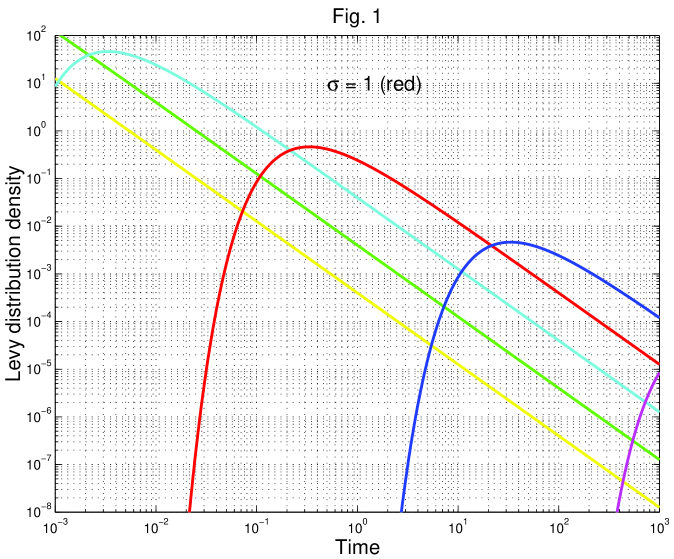
Plot of PDFs for the Lévy distribution (2), .
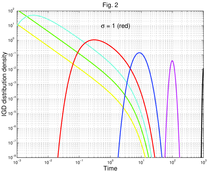
Plot of PDFs for the IGD distribution (4), .
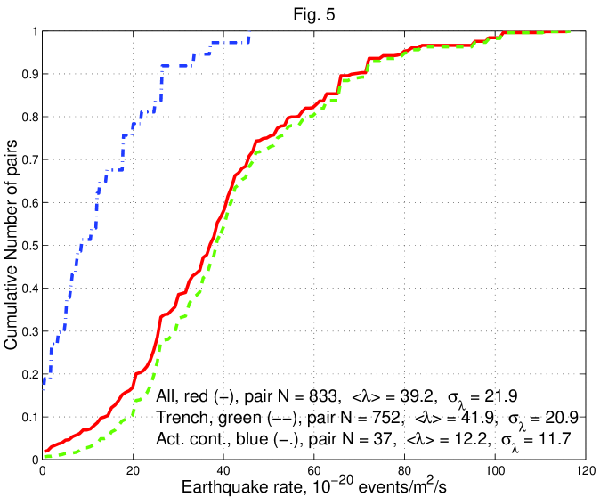
Normalized cumulative distribution of earthquake rate for shallow earthquake pairs in all zones, trench (subduction) zones, and active continental zones. The pair numbers , average rate and its standard deviation are also shown. Earthquake rate is taken from a table by Bird et al. (2010) for a magnitude threshold .
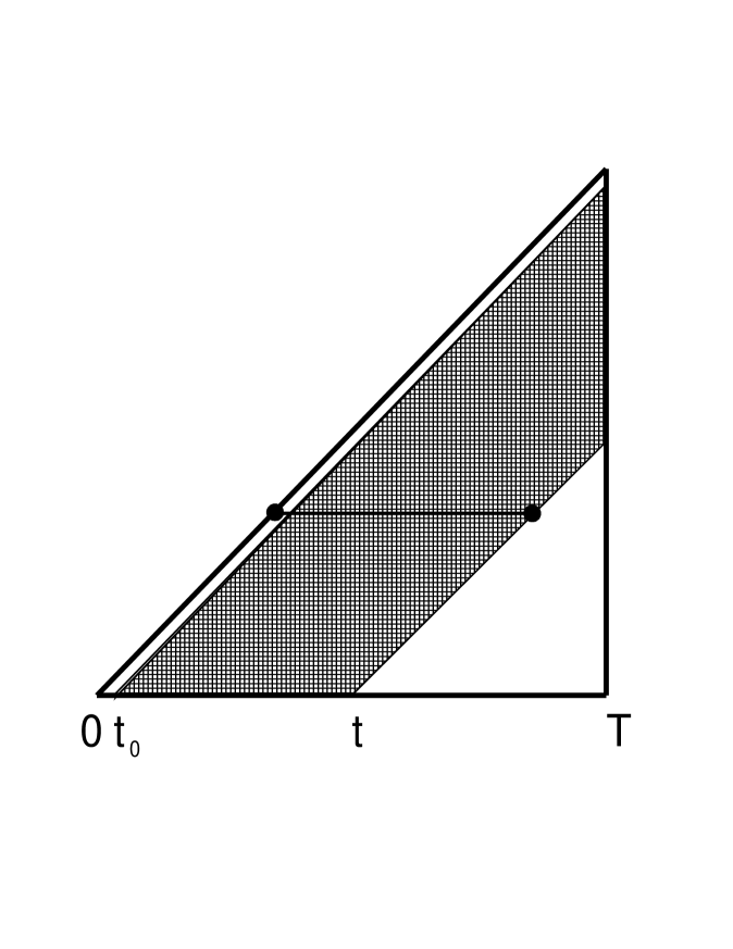
Integration domain for calculating inter-earthquake rates in a catalog of duration . The minimum time interval, , corresponds to the coda duration time of the first event.
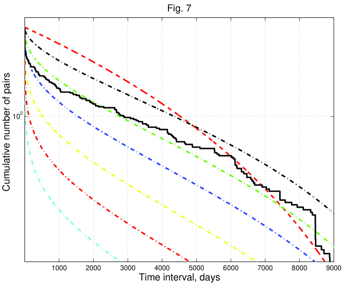
Earthquake pair numbers in all zones with rates events/m2/s. Earthquake rate is taken from a table by Bird et al. (2010) for a magnitude threshold . Pair number is 240. Solid curve is earthquake pair numbers; dashed curve is Poisson approximation (15), dash-dotted curves are for power-law approximations (16), the -value is 0.5, 0.65, 0.75, 0.85, 0.925, and 0.99 from top to bottom. The catalogs time interval is 1976/1/1–2010/11/14. Average recurrence time () for earthquakes is days.
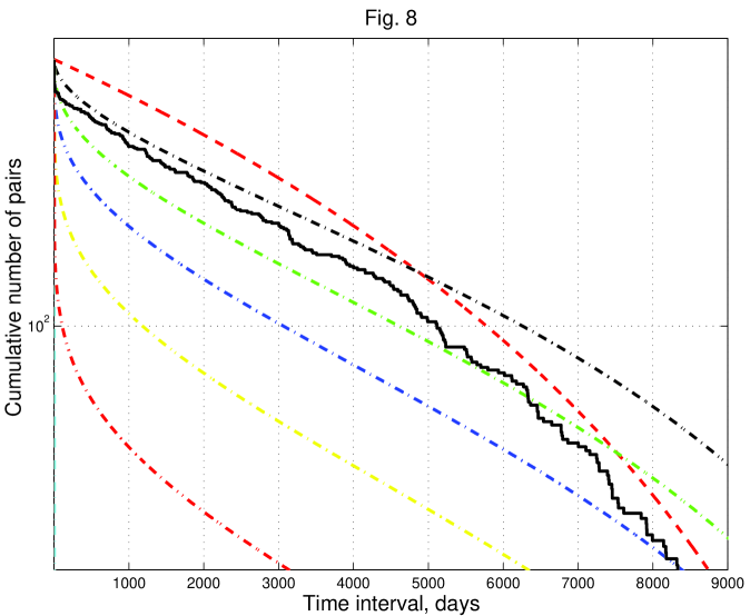
Earthquake pair numbers in all zones with rates events/m2/s. Pair number is 333. Average recurrence time () for earthquakes is days. For notation see Fig. 7.
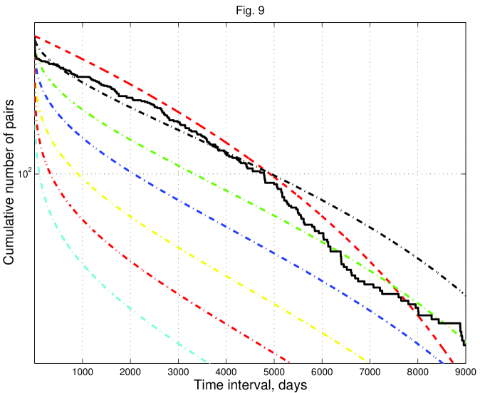
Earthquake pair numbers in all zones with rates events/m2/s. Pair number is 264. Average recurrence time () for earthquakes is days. For notation see Fig. 7.
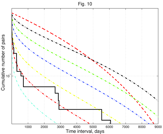
Earthquake pair numbers in active continental zones. Pair number is 37. Average recurrence time () for earthquakes is days. For notation see Fig. 7.
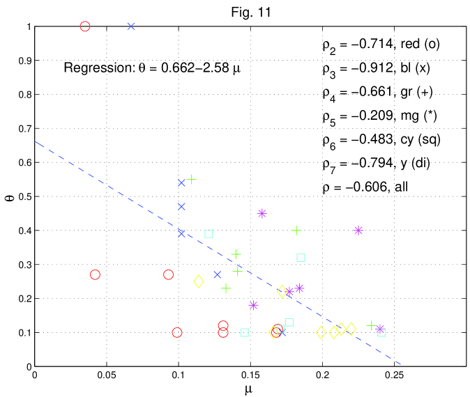
Correlation between maximum likelihood estimates of and parameters in several earthquake catalogs (Kagan et al., 2010). The subscripts at correlation coefficients () point to the table number in Kagan et al. (2010).
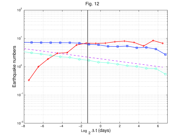
The average aftershock numbers from the PDE catalog in logarithmic time intervals following GCMT earthquakes during 1977-2003. Line with plus signs shows aftershocks; dashed lines are theoretical estimates for the first generation aftershocks. Two curves display results of earthquake catalog simulation: line with circles shows first generation aftershocks, line with squares indicates total aftershock numbers.
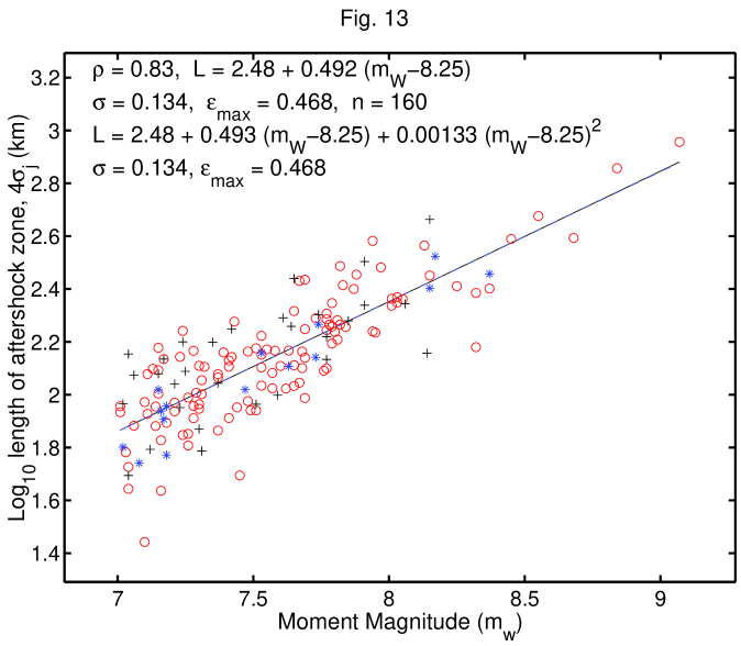
Plot of log aftershock zone length () against moment magnitude (). Rupture length is determined using a 1-day aftershock pattern. Values of the correlation coefficient (), coefficients for linear (dashed line) and quadratic (solid line) regression, standard () and maximum () errors, and the total number () of aftershock sequences are shown in the diagram. Circles – thrust mainshocks; Stars – normal mainshocks; Pluses – strike-slip mainshocks.
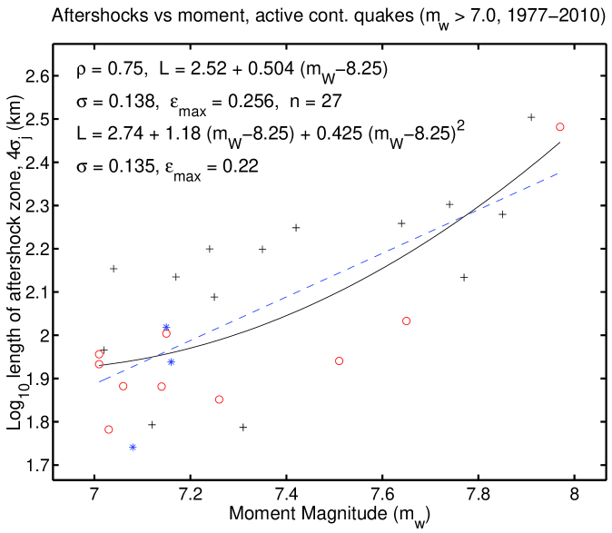
Plot of log aftershock zone length () against moment magnitude () for earthquakes in active continental zones (Kagan et al., 2010). For notation see Fig. 13.