Optimal mean-variance investment strategy under value-at-risk constraints

Jun Ye Department of Mathematical Sciences, Tsinghua University Beijing, 100084, China. jye@math.tsinghua.edu.cn Tiantian Li 111Tel.:+86-10-66931968 litt08@mails.tsinghua.edu.cn
Abstract

This paper is devoted to study the effects arising from imposing a value-at-risk (VaR) constraint in mean-variance portfolio selection problem for an investor who receives a stochastic cash flow which he/she must then invest in a continuous-time financial market. For simplicity, we assume that there is only one investment opportunity available for the investor, a risky stock. Using techniques of stochastic linear-quadratic (LQ) control, the optimal mean-variance investment strategy with and without VaR constraint are derived explicitly in closed forms, based on solution of corresponding Hamilton-Jacobi-Bellman (HJB) equation. Furthermore, some numerical examples are proposed to show how the addition of the VaR constraint affects the optimal strategy.

keywords:
Value-at-risk , Mean-variance portfolio , Hamilton-Jacobi-Bellman equation , Optimal investment strategy.
MSC:
C02 , C61 , IM01.
journal: Insurance: Mathematics and Economics

1 Introduction

The mean-variance model of Markowitz (1952, 1959) is a cornerstone of modern portfolio theory. The most important contribution of this model is that it enables an investor to optimally select mean-variance efficient portfolios for seeking the highest return after specifying his acceptable risk level. Since Markowitz’s pioneering work, the mean-variance model was extended from single-period case to multi-period discrete-time case (see Hakansson, 1971; Pliska, 1997; Samuelson, 1969, etc.) and continuous time case during the last decades (see Cox and Huang, 1989; Duffie and Richardson, 1991; Karatzas et al., 1987; Schweizer, 1996, etc.). However, when studying these two kinds of dynamic portfolio selection models, most research works have been dominated by those of maximizing expected utility functions of the terminal wealth. Nevertheless, when using this approach, the tradeoff information between the risk and the expected return is implicit, which makes the investment decision less intuitive. In 2000, Zhou and Li introduce the stochastic linear-quadratic (LQ) control as a general framework to study the mean-variance optimization problem. Within this framework they have established a natural connection of the portfolio selection problems and standard stochastic control models and attained some elegant results for a continuous-time mean-variance model with determined coefficients.

When using stochastic LQ control approach to deal with continuous time mean-variance problem, the terminal wealth is a random variable with a distribution that is often extremely skewed and shows considerable probability in regions of small values of the terminal wealth. This means that the optimal terminal wealth may exhibit large shortfall risks. In order to prevent investors from extremely dangerous positions in the market, it is thus more reasonable to consider asymmetric risk measures, e.g. value-at-risk (VaR), to limit the exposure to market risks.

In market risk management, it is widely accepted that VaR is a useful summary measure of market risks which regulatory authorities sometimes enforced investors to use. VaR is actually the maximum expected loss over a given horizon period at a given level of confidence. For comprehensive introduction to risk management using VaR, we refer the reader to Jorion (1997).

Recognizing that risk management is typically not an investor’s primary objective, the investors would like to limit their risks while maximizing expected utility. This leads to stochastic control problems under restrictions on such risk measures. There has been considerable interest in the study of portfolio selection models subject to a VaR constraint. Kluppelberg and Korn (1998), Alexander and Baptista (2004, 2007) investigate the optimal portfolio choices subject to a VaR or conditional VaR (CVaR) constraint in a static (one-period) setting. The similar problems in a dynamic setting has started to draw more attentions recently, Basak and Shapiro (2001) focus on the optimal portfolio policies of a utility-maximizing agent by imposing the VaR constraint at one point in time. Cuoco et al. (2008) developed a realistic dynamically consistent model of the optimal behavior of a trader subject to risk constraints. They assume that the risk of the trading portfolio is re-evaluated dynamically by using the conditioning information, and hence the trader must satisfy the risk limit continuously. Yiu (2004) explicitly derived the standard VaR constraint on total wealth and obtained optimal trading strategy(without consideration of re-insurance). Pirvu (2005) started with the model of Cuoco et al. (2008) and found the optimal growth portfolio subject to these risk measures. Pirvu (2007) extended those results by extensively studying the optimal investment and consumption strategies for both logarithmic utility and non-logarithmic CRRA utilities.

Motivated by Zhou and Li (2000) and Yiu (2004), this paper addresses the problem of an investor who receives an uncontrollable stochastic cash flow which he must then invest in a complete continuous-time financial market in order to maximize the weighted average of the expectation and the variance of his terminal wealth at a horizon time. The main focus in this paper is on the mean-variance optimization problem of the investor subject to a risk limit specified in terms of VaR on his future net worth. To our knowledge, this problem has not yet received a complete treatment in the existing literature. In this paper, we derive the optimal mean-variance investment strategy under a standard VaR constraint by solving the corresponding Hamilton-Jacobi-Bellman (HJB) equation and explore how the addition of a risk constraint affects the optimal solution.

The rest of the paper is organized as follows. Section 2 describes the model, including the definition of the VaR on the future net worth process. Section 3 contains the main characterization result of the VaR constraint and formulates the portfolio optimization problem that can be eventually discussed as a stochastic LQ problem. Section 4 gives the explicit solution of the optimal mean-variance strategy without VaR constraint by solving the corresponding HJB equation. Section 5 discusses the optimal mean-variance strategy with VaR constraint. Finally, Section 6 provides some numerical examples to show how the addition of the VaR constraint affects the optimal strategy.

2 The Model

2.1 Continuous-time investment in stochastic cash flow

All stochastic processes introduced below are supposed to be adapted in a filtered probability space (Ω,,t,P)Ωsubscript𝑡𝑃(\Omega,\mathcal{F},\mathcal{F}_{t},P), where t,t0subscript𝑡𝑡0\mathcal{F}_{t},t\geq 0 is a filtration satisfying the usual conditions. Moreover, it is assumed throughout this paper that all inequalities as well as equalities hold P𝑃P-almost surely.

Following the framework of Browne (1995), for simplicity, and without any loss of generality, we assume that there is only one risky stock available for investment, whose price at time t𝑡t will be denoted by Ptsubscript𝑃𝑡P_{t} which satisfies the following stochastic differential equation

dPt=Pt(μdt+σdWt(1)),𝑑subscript𝑃𝑡subscript𝑃𝑡𝜇𝑑𝑡𝜎𝑑superscriptsubscript𝑊𝑡1dP_{t}=P_{t}(\mu dt+\sigma dW_{t}^{(1)}), (1)

where μ>0𝜇0\mu>0 is the appreciation rate and σ>0𝜎0\sigma>0 is the volatility or the dispersion of the stock. Wt(1)superscriptsubscript𝑊𝑡1W_{t}^{(1)} is a standard Brownian motion.

Since we are concerned with investment behavior in the presence of a stochastic cash flow, or an external risk process denoted by Ytsubscript𝑌𝑡Y_{t}, which is another Browian motion with drift α𝛼\alpha and diffusion parameter β>0𝛽0\beta>0, that is

dYt=αdt+βdWt(2),𝑑subscript𝑌𝑡𝛼𝑑𝑡𝛽𝑑superscriptsubscript𝑊𝑡2dY_{t}=\alpha dt+\beta dW_{t}^{(2)}, (2)

where Wt(1)superscriptsubscript𝑊𝑡1W_{t}^{(1)} and Wt(2)superscriptsubscript𝑊𝑡2W_{t}^{(2)} are possibly correlated with correlation coefficient ρ𝜌\rho. In case there would only be one source of randomness left in the model, we also assume that ρ2<1superscript𝜌21\rho^{2}<1.

We will define an investment strategy f𝑓f as an admissible adapted control process ftsubscript𝑓𝑡f_{t}, satisfying that 0Tft2𝑑t<superscriptsubscript0𝑇superscriptsubscript𝑓𝑡2differential-d𝑡\int_{0}^{T}f_{t}^{2}dt<\infty, a.s., for all T<𝑇T<\infty. Note that ftsubscript𝑓𝑡f_{t} represents the amount invested in risky stock at time t𝑡t, and we will not put more constraints on ftsubscript𝑓𝑡f_{t}. In particular, we will allow ft<0subscript𝑓𝑡0f_{t}<0, which means short-selling would be allowed, the circumstance that ft>Xtfsubscript𝑓𝑡superscriptsubscript𝑋𝑡𝑓f_{t}>X_{t}^{f} is also permitted so that the investor can borrow money to buy stock.

Assume that the trading takes place continuously and transaction cost is not considered. Therefore, following the investment strategy f𝑓f, the wealth process of the investor at time t𝑡t , which will be denoted by Xtfsuperscriptsubscript𝑋𝑡𝑓X_{t}^{f}, can be given by the following stochastic differential equation with initial condition X0=xsubscript𝑋0𝑥X_{0}=x

dXt=(ftμ+α)dt+ftσdWt(1)+βdWt(2),X0=x.formulae-sequence𝑑subscript𝑋𝑡subscript𝑓𝑡𝜇𝛼𝑑𝑡subscript𝑓𝑡𝜎𝑑superscriptsubscript𝑊𝑡1𝛽𝑑superscriptsubscript𝑊𝑡2subscript𝑋0𝑥dX_{t}=(f_{t}\mu+\alpha)dt+f_{t}\sigma dW_{t}^{(1)}+\beta dW_{t}^{(2)},X_{0}=x. (3)

2.2 Value-at-risk

Now we want to introduce the definition of value-at-risk. Here we start by rewriting (3) into integration form

Xtf=x+0t(fsμ+α)𝑑s+0t(fsσ)𝑑Ws(1)+0tβ𝑑Ws(2),superscriptsubscript𝑋𝑡𝑓𝑥superscriptsubscript0𝑡subscript𝑓𝑠𝜇𝛼differential-d𝑠superscriptsubscript0𝑡subscript𝑓𝑠𝜎differential-dsuperscriptsubscript𝑊𝑠1superscriptsubscript0𝑡𝛽differential-dsuperscriptsubscript𝑊𝑠2X_{t}^{f}=x+\int_{0}^{t}(f_{s}\mu+\alpha)ds+\int_{0}^{t}(f_{s}\sigma)dW_{s}^{(1)}+\int_{0}^{t}\beta dW_{s}^{(2)}, (4)

where x>0𝑥0x>0 denotes the initial value of the portfolio. Notice that (4) leads to

Xt+τf=Xt+tt+τ(fsμ+α)𝑑s+tt+τ(fsσ)𝑑Ws(1)+tt+τβ𝑑Ws(2),superscriptsubscript𝑋𝑡𝜏𝑓subscript𝑋𝑡superscriptsubscript𝑡𝑡𝜏subscript𝑓𝑠𝜇𝛼differential-d𝑠superscriptsubscript𝑡𝑡𝜏subscript𝑓𝑠𝜎differential-dsuperscriptsubscript𝑊𝑠1superscriptsubscript𝑡𝑡𝜏𝛽differential-dsuperscriptsubscript𝑊𝑠2X_{t+\tau}^{f}=X_{t}+\int_{t}^{t+\tau}(f_{s}\mu+\alpha)ds+\int_{t}^{t+\tau}(f_{s}\sigma)dW_{s}^{(1)}+\int_{t}^{t+\tau}\beta dW_{s}^{(2)}, (5)

for any τ>0𝜏0\tau>0.

If we assume that the investment strategy were kept constant during the time period (t,t+τ]𝑡𝑡𝜏(t,t+\tau], i.e. fsfsubscript𝑓𝑠𝑓f_{s}\equiv f, for any s(t,t+τ]𝑠𝑡𝑡𝜏s\in(t,t+\tau], then it follows immediately from (5) that, given the strategy f𝑓f and the associated wealth value Xt=Xsubscript𝑋𝑡𝑋X_{t}=X at time t𝑡t, the random variable 𝒳t+τ(X,f)subscript𝒳𝑡𝜏𝑋𝑓\mathcal{X}_{t+\tau}(X,f) would be the future value of the wealth at time t+τ𝑡𝜏t+\tau

𝒳t+τ(X,f)=Xt+(fμ+α)τ+fσ(Wt+τ(1)Wt(1))+β(Wt+τ(2)Wt(2)).subscript𝒳𝑡𝜏𝑋𝑓subscript𝑋𝑡𝑓𝜇𝛼𝜏𝑓𝜎superscriptsubscript𝑊𝑡𝜏1superscriptsubscript𝑊𝑡1𝛽superscriptsubscript𝑊𝑡𝜏2superscriptsubscript𝑊𝑡2\mathcal{X}_{t+\tau}(X,f)=X_{t}+(f\mu+\alpha)\tau+f\sigma(W_{t+\tau}^{(1)}-W_{t}^{(1)})+\beta(W_{t+\tau}^{(2)}-W_{t}^{(2)}). (6)

Therefore we define the future net worth of the wealth process in horizon period (t,t+τ]𝑡𝑡𝜏(t,t+\tau] by 𝒳t+τ(X,f)Xtsubscript𝒳𝑡𝜏𝑋𝑓subscript𝑋𝑡\mathcal{X}_{t+\tau}(X,f)-X_{t}.

Definition 1 (Value-at-risk).

Given a probability level p(0,1)𝑝01p\in(0,1) and a horizon τ>0𝜏0\tau>0, the value-at-risk of the future net worth of the wealth process with investment strategy f𝑓f at time t𝑡t, denoted by VaRtp,f𝑉𝑎superscriptsubscript𝑅𝑡𝑝𝑓VaR_{t}^{p,f}, is defined as

VaRtp,f=(Qtp,f),𝑉𝑎superscriptsubscript𝑅𝑡𝑝𝑓superscriptsuperscriptsubscript𝑄𝑡𝑝𝑓VaR_{t}^{p,f}=(Q_{t}^{p,f})^{-}, (7)

where

Qtp,f=sup{L:P(𝒳t+τXtLt)<p},superscriptsubscript𝑄𝑡𝑝𝑓𝑠𝑢𝑝conditional-set𝐿𝑃subscript𝒳𝑡𝜏subscript𝑋𝑡conditional𝐿subscript𝑡𝑝Q_{t}^{p,f}=sup\{L\in\mathbb{R}:P(\mathcal{X}_{t+\tau}-X_{t}\leq L\mid\mathcal{F}_{t})<p\}, (8)

and x=max{0,x}.superscript𝑥𝑚𝑎𝑥0𝑥x^{-}=max\{0,-x\}.

Consequently, Qtp,fsuperscriptsubscript𝑄𝑡𝑝𝑓Q_{t}^{p,f} is the plimit-from𝑝p-quantile of the projected portfolio gain over the time interval (t,t+τ]𝑡𝑡𝜏(t,t+\tau]. In other words, VaRtp,f𝑉𝑎superscriptsubscript𝑅𝑡𝑝𝑓VaR_{t}^{p,f} is the greatest loss over the next period of length τ𝜏\tau which would be exceeded only with a small conditional probability p𝑝p if the current portfolio ftsubscript𝑓𝑡f_{t} were kept the same.

Proposition 1 (Computation of value-at-risk).

We have

VaRtp,f=(Qtp,f)=(τ(fμ+α)+τf2σ2+β2+2ρσβfΦ1(p)),𝑉𝑎superscriptsubscript𝑅𝑡𝑝𝑓superscriptsuperscriptsubscript𝑄𝑡𝑝𝑓superscript𝜏𝑓𝜇𝛼𝜏superscript𝑓2superscript𝜎2superscript𝛽22𝜌𝜎𝛽𝑓superscriptΦ1𝑝VaR_{t}^{p,f}=(Q_{t}^{p,f})^{-}=(\tau(f\mu+\alpha)+\sqrt{\tau}\sqrt{f^{2}\sigma^{2}+\beta^{2}+2\rho\sigma\beta f}\Phi^{-1}(p))^{-}, (9)

where Φ()Φ\Phi(\cdot) and Φ1()superscriptΦ1\Phi^{-1}(\cdot) denote the standard normal distribution and inverse distribution functions respectively.

Proof of Proposition 1.

We have

P(𝒳t+τXtLt)𝑃subscript𝒳𝑡𝜏subscript𝑋𝑡conditional𝐿subscript𝑡\displaystyle P(\mathcal{X}_{t+\tau}-X_{t}\leq L\mid\mathcal{F}_{t})
=\displaystyle= P((fμ+α)τ+fσ(Wt+τ(1)Wt(1))+β(Wt+τ(2)Wt(2))Lt)𝑃𝑓𝜇𝛼𝜏𝑓𝜎superscriptsubscript𝑊𝑡𝜏1superscriptsubscript𝑊𝑡1𝛽superscriptsubscript𝑊𝑡𝜏2superscriptsubscript𝑊𝑡2conditional𝐿subscript𝑡\displaystyle P((f\mu+\alpha)\tau+f\sigma(W_{t+\tau}^{(1)}-W_{t}^{(1)})+\beta(W_{t+\tau}^{(2)}-W_{t}^{(2)})\leq L\mid\mathcal{F}_{t})
=\displaystyle= P(fσ(Wt+τ(1)Wt(1))+β(Wt+τ(2)Wt(2))L(fμ+α)τt)𝑃𝑓𝜎superscriptsubscript𝑊𝑡𝜏1superscriptsubscript𝑊𝑡1𝛽superscriptsubscript𝑊𝑡𝜏2superscriptsubscript𝑊𝑡2𝐿conditional𝑓𝜇𝛼𝜏subscript𝑡\displaystyle P(f\sigma(W_{t+\tau}^{(1)}-W_{t}^{(1)})+\beta(W_{t+\tau}^{(2)}-W_{t}^{(2)})\leq L-(f\mu+\alpha)\tau\mid\mathcal{F}_{t})
=\displaystyle= P(ZL(fμ+α)ττf2σ2+β2+2ρσβft)𝑃𝑍conditional𝐿𝑓𝜇𝛼𝜏𝜏superscript𝑓2superscript𝜎2superscript𝛽22𝜌𝜎𝛽𝑓subscript𝑡\displaystyle P(Z\leq\frac{L-(f\mu+\alpha)\tau}{\sqrt{\tau}\sqrt{f^{2}\sigma^{2}+\beta^{2}+2\rho\sigma\beta f}}\mid\mathcal{F}_{t})
=\displaystyle= Φ(L(fμ+α)ττf2σ2+β2+2ρσβf),Φ𝐿𝑓𝜇𝛼𝜏𝜏superscript𝑓2superscript𝜎2superscript𝛽22𝜌𝜎𝛽𝑓\displaystyle\Phi(\frac{L-(f\mu+\alpha)\tau}{\sqrt{\tau}\sqrt{f^{2}\sigma^{2}+\beta^{2}+2\rho\sigma\beta f}}),

where Z=fσ(Wt+τ(1)Wt(1))+β(Wt+τ(2)Wt(2))τf2σ2+β2+2ρσβf𝑍𝑓𝜎superscriptsubscript𝑊𝑡𝜏1superscriptsubscript𝑊𝑡1𝛽superscriptsubscript𝑊𝑡𝜏2superscriptsubscript𝑊𝑡2𝜏superscript𝑓2superscript𝜎2superscript𝛽22𝜌𝜎𝛽𝑓Z=\frac{f\sigma(W_{t+\tau}^{(1)}-W_{t}^{(1)})+\beta(W_{t+\tau}^{(2)}-W_{t}^{(2)})}{\sqrt{\tau}\sqrt{f^{2}\sigma^{2}+\beta^{2}+2\rho\sigma\beta f}} follows standard normal distribution conditionally. Thus, from

P(𝒳t+τXtLt)<p,𝑃subscript𝒳𝑡𝜏subscript𝑋𝑡conditional𝐿subscript𝑡𝑝P(\mathcal{X}_{t+\tau}-X_{t}\leq L\mid\mathcal{F}_{t})<p,

we know that

Φ(L(fμ+α)ττf2σ2+β2+2ρσβf)<p,Φ𝐿𝑓𝜇𝛼𝜏𝜏superscript𝑓2superscript𝜎2superscript𝛽22𝜌𝜎𝛽𝑓𝑝\Phi(\frac{L-(f\mu+\alpha)\tau}{\sqrt{\tau}\sqrt{f^{2}\sigma^{2}+\beta^{2}+2\rho\sigma\beta f}})<p,

which gives rise to

L<τ(fμ+α)+τf2σ2+β2+2ρσβfΦ1(p).𝐿𝜏𝑓𝜇𝛼𝜏superscript𝑓2superscript𝜎2superscript𝛽22𝜌𝜎𝛽𝑓superscriptΦ1𝑝L<\tau(f\mu+\alpha)+\sqrt{\tau}\sqrt{f^{2}\sigma^{2}+\beta^{2}+2\rho\sigma\beta f}\Phi^{-1}(p).

And therefore

Qtp,fsuperscriptsubscript𝑄𝑡𝑝𝑓\displaystyle Q_{t}^{p,f} =\displaystyle= sup{L:L<τ(fμ+α)+τf2σ2+β2+2ρσβfΦ1(p)}𝑠𝑢𝑝conditional-set𝐿𝐿𝜏𝑓𝜇𝛼𝜏superscript𝑓2superscript𝜎2superscript𝛽22𝜌𝜎𝛽𝑓superscriptΦ1𝑝\displaystyle sup\{L\in\mathbb{R}:L<\tau(f\mu+\alpha)+\sqrt{\tau}\sqrt{f^{2}\sigma^{2}+\beta^{2}+2\rho\sigma\beta f}\Phi^{-1}(p)\}
=\displaystyle= τ(fμ+α)+τf2σ2+β2+2ρσβfΦ1(p),𝜏𝑓𝜇𝛼𝜏superscript𝑓2superscript𝜎2superscript𝛽22𝜌𝜎𝛽𝑓superscriptΦ1𝑝\displaystyle\tau(f\mu+\alpha)+\sqrt{\tau}\sqrt{f^{2}\sigma^{2}+\beta^{2}+2\rho\sigma\beta f}\Phi^{-1}(p),

which immediately gives (9). ∎

Note that even when f0𝑓0f\equiv 0, which means there is no investment in risky stock, VaRtp,0=τ(α+βΦ1(p)/τ)𝑉𝑎superscriptsubscript𝑅𝑡𝑝0𝜏𝛼𝛽superscriptΦ1𝑝𝜏VaR_{t}^{p,0}=\tau(\alpha+\beta\Phi^{-1}(p)/\sqrt{\tau}) is also positive if α/β<Φ1(1p)/τ𝛼𝛽superscriptΦ11𝑝𝜏\alpha/\beta<\Phi^{-1}(1-p)/\sqrt{\tau}. This results from the incompleteness of the model, in which the cash flow Y𝑌Y cannot be traded and therefore the risk cannot be eliminated as long as ρ2<1superscript𝜌21\rho^{2}<1.

3 Statement of the Problem

We consider the optimal control problem of the investor who starts with an initial wealth X0=xsubscript𝑋0𝑥X_{0}=x and must select a strategy f𝑓f so as to maximize the weighted average of the expectation and the variance of his terminal wealth, subjected to the constraint that the VaR with the chosen portfolio is no larger than a given level VaR¯¯𝑉𝑎𝑅\overline{VaR} at any time t[0,T]𝑡0𝑇t\in[0,T]. In mathematical terms, this problem can be described as

supfE[XTfγ(XTf)2]s.t.dXt=(ftμ+α)dt+ftσdWt(1)+βdWt(2),X0=x,VaRtp,fVaR¯,t[0,T].subscriptsupremum𝑓𝐸delimited-[]superscriptsubscript𝑋𝑇𝑓𝛾superscriptsuperscriptsubscript𝑋𝑇𝑓2formulae-sequences.t.𝑑subscript𝑋𝑡subscript𝑓𝑡𝜇𝛼𝑑𝑡subscript𝑓𝑡𝜎𝑑superscriptsubscript𝑊𝑡1𝛽𝑑superscriptsubscript𝑊𝑡2subscript𝑋0𝑥formulae-sequence𝑉𝑎superscriptsubscript𝑅𝑡𝑝𝑓¯𝑉𝑎𝑅for-all𝑡0𝑇\begin{array}[]{c}\sup\limits_{f}E[X_{T}^{f}-\gamma(X_{T}^{f})^{2}]\\ \textrm{s.t.}\qquad dX_{t}=(f_{t}\mu+\alpha)dt+f_{t}\sigma dW_{t}^{(1)}+\beta dW_{t}^{(2)},X_{0}=x,\\ VaR_{t}^{p,f}\leq\overline{VaR},\forall t\in[0,T].\end{array} (10)

where the parameter (representing the weight) γ𝛾\gamma is positive. We denote the optimal solution of problem (10) by fVaRsuperscriptsubscript𝑓𝑉𝑎𝑅f_{VaR}^{*} if it exists. Note that the upper bound VaR¯¯𝑉𝑎𝑅\overline{VaR} can be dependent on Xtfsuperscriptsubscript𝑋𝑡𝑓X_{t}^{f} and t𝑡t, however in this paper, we set VaR¯¯𝑉𝑎𝑅\overline{VaR} to be a constant in order to obtain the explicit solution.

Proposition 2 (Computation of the value-at-risk constraint).

The explicit form of the VaR constraint in problem(10) is

{[M2N2β22μ(ρβNM),+),if Nσ=μ,ρβN<M,[f1,+),if Nσ<μ,[f2,f1],if 0<N2σ2μ2(σMρβμ)2(1ρ2)β2,ρβμ<σM,,otherwise,casessuperscript𝑀2superscript𝑁2superscript𝛽22𝜇𝜌𝛽𝑁𝑀if Nσ=μ,ρβN<M,subscript𝑓1if Nσ<μ,subscript𝑓2subscript𝑓1formulae-sequenceif 0superscript𝑁2superscript𝜎2superscript𝜇2superscript𝜎𝑀𝜌𝛽𝜇21superscript𝜌2superscript𝛽2𝜌𝛽𝜇𝜎𝑀otherwise\left\{\begin{array}[]{ll}[\frac{M^{2}-N^{2}\beta^{2}}{2\mu(\rho\beta N-M)},+\infty),&\textrm{if $N\sigma=\mu,\rho\beta N<M$,}\\ [f_{1},+\infty),&\textrm{if $N\sigma<\mu$,}\\ [f_{2},f_{1}],&\textrm{if }0<N^{2}\sigma^{2}-\mu^{2}\leq\frac{(\sigma M-\rho\beta\mu)^{2}}{(1-\rho^{2})\beta^{2}},\rho\beta\mu<\sigma M,\\ \emptyset,&\textrm{otherwise},\end{array}\right. (11)

where N=Φ1(1p)/τ>0𝑁superscriptΦ11𝑝𝜏0N=\Phi^{-1}(1-p)/\sqrt{\tau}>0, M=α+VaR¯/τ>0𝑀𝛼¯𝑉𝑎𝑅𝜏0M=\alpha+\overline{VaR}/\tau>0, and

f1,2=2(μMρσβN2)±Δ2(N2σ2μ2),subscript𝑓12plus-or-minus2𝜇𝑀𝜌𝜎𝛽superscript𝑁2Δ2superscript𝑁2superscript𝜎2superscript𝜇2f_{1,2}=\frac{2(\mu M-\rho\sigma\beta N^{2})\pm\sqrt{\Delta}}{2(N^{2}\sigma^{2}-\mu^{2})}, (12)

if Δ=4N2((1ρ2)β2(μ2N2σ2)+(σMρβμ)2)0Δ4superscript𝑁21superscript𝜌2superscript𝛽2superscript𝜇2superscript𝑁2superscript𝜎2superscript𝜎𝑀𝜌𝛽𝜇20\Delta=4N^{2}((1-\rho^{2})\beta^{2}(\mu^{2}-N^{2}\sigma^{2})+(\sigma M-\rho\beta\mu)^{2})\geq 0 and N2σ2μ2superscript𝑁2superscript𝜎2superscript𝜇2N^{2}\sigma^{2}\neq\mu^{2}. We also assume that f1subscript𝑓1f_{1} is always larger than f2subscript𝑓2f_{2}.

Proof of Proposition 2.

The VaR constraint can be written as

τ(fμ+α+Φ1(p)τf2σ2+β2+2ρσβf)VaR¯,𝜏superscript𝑓𝜇𝛼superscriptΦ1𝑝𝜏superscript𝑓2superscript𝜎2superscript𝛽22𝜌𝜎𝛽𝑓¯𝑉𝑎𝑅\tau(f\mu+\alpha+\frac{\Phi^{-1}(p)}{\sqrt{\tau}}\sqrt{f^{2}\sigma^{2}+\beta^{2}+2\rho\sigma\beta f})^{-}\leq\overline{VaR},

which is equivalent to

{(Φ1(p)τ)2(f2σ2+β2+2ρσβf)(fμ+α+VaR¯τ)2,fμ+α+VaR¯τ0,casessuperscriptsuperscriptΦ1𝑝𝜏2superscript𝑓2superscript𝜎2superscript𝛽22𝜌𝜎𝛽𝑓superscript𝑓𝜇𝛼¯𝑉𝑎𝑅𝜏2𝑓𝜇𝛼¯𝑉𝑎𝑅𝜏0\left\{\begin{array}[]{l}(\frac{\Phi^{-1}(p)}{\sqrt{\tau}})^{2}(f^{2}\sigma^{2}+\beta^{2}+2\rho\sigma\beta f)\leq(f\mu+\alpha+\frac{\overline{VaR}}{\tau})^{2},\\ f\mu+\alpha+\frac{\overline{VaR}}{\tau}\geq 0,\end{array}\right.

that is, after some simplifications,

{N2(f2σ2+β2+2ρσβf)(fμ+M)2,fμ+M0,casessuperscript𝑁2superscript𝑓2superscript𝜎2superscript𝛽22𝜌𝜎𝛽𝑓superscript𝑓𝜇𝑀2𝑓𝜇𝑀0\left\{\begin{array}[]{l}N^{2}(f^{2}\sigma^{2}+\beta^{2}+2\rho\sigma\beta f)\leq(f\mu+M)^{2},\\ f\mu+M\geq 0,\end{array}\right.

where N=Φ1(1p)/τ>0𝑁superscriptΦ11𝑝𝜏0N=\Phi^{-1}(1-p)/\sqrt{\tau}>0, M=α+VaR¯/τ>0𝑀𝛼¯𝑉𝑎𝑅𝜏0M=\alpha+\overline{VaR}/\tau>0. Note that when f=M/μ𝑓𝑀𝜇f=-M/\mu, N2(f2σ2+β2+2ρσβf)>0=(fμ+M)2superscript𝑁2superscript𝑓2superscript𝜎2superscript𝛽22𝜌𝜎𝛽𝑓0superscript𝑓𝜇𝑀2N^{2}(f^{2}\sigma^{2}+\beta^{2}+2\rho\sigma\beta f)>0=(f\mu+M)^{2} always holds. This observation will help us in the second case when N2σ2μ2<0superscript𝑁2superscript𝜎2superscript𝜇20N^{2}\sigma^{2}-\mu^{2}<0 and the third case when N2σ2μ2>0superscript𝑁2superscript𝜎2superscript𝜇20N^{2}\sigma^{2}-\mu^{2}>0.

Therefore we have a group of inequalities

{(N2σ2μ2)f2+2(ρσβN2μM)f+(N2β2M2)0,fM/μ.casessuperscript𝑁2superscript𝜎2superscript𝜇2superscript𝑓22𝜌𝜎𝛽superscript𝑁2𝜇𝑀𝑓superscript𝑁2superscript𝛽2superscript𝑀20𝑓𝑀𝜇\left\{\begin{array}[]{l}(N^{2}\sigma^{2}-\mu^{2})\cdot f^{2}+2(\rho\sigma\beta N^{2}-\mu M)\cdot f+(N^{2}\beta^{2}-M^{2})\leq 0,\\ f\geq-M/\mu.\end{array}\right. (13)

First we study the degeneration case: N2σ2μ2=0superscript𝑁2superscript𝜎2superscript𝜇20N^{2}\sigma^{2}-\mu^{2}=0,i.e. Nσ=μ𝑁𝜎𝜇N\sigma=\mu.

In this case, if 2(ρσβN2μM)>02𝜌𝜎𝛽superscript𝑁2𝜇𝑀02(\rho\sigma\beta N^{2}-\mu M)>0, i.e. ρβN>M𝜌𝛽𝑁𝑀\rho\beta N>M, then the first inequality of (13) would imply

fM2N2β22(ρσβN2μM)=M2N2β22μ(ρβNM),𝑓superscript𝑀2superscript𝑁2superscript𝛽22𝜌𝜎𝛽superscript𝑁2𝜇𝑀superscript𝑀2superscript𝑁2superscript𝛽22𝜇𝜌𝛽𝑁𝑀f\leq\frac{M^{2}-N^{2}\beta^{2}}{2(\rho\sigma\beta N^{2}-\mu M)}=\frac{M^{2}-N^{2}\beta^{2}}{2\mu(\rho\beta N-M)},

however

Mμ>M2N2β22μ(ρβNM),𝑀𝜇superscript𝑀2superscript𝑁2superscript𝛽22𝜇𝜌𝛽𝑁𝑀-\frac{M}{\mu}>\frac{M^{2}-N^{2}\beta^{2}}{2\mu(\rho\beta N-M)},

which, together with the second inequality of (13), leads to f𝑓f\in\emptyset.

If 2(ρσβN2μM)=02𝜌𝜎𝛽superscript𝑁2𝜇𝑀02(\rho\sigma\beta N^{2}-\mu M)=0, i.e. ρβN=M𝜌𝛽𝑁𝑀\rho\beta N=M, then the first inequality of (13) would imply

N2β2M2=N2β2(1ρ2)0,superscript𝑁2superscript𝛽2superscript𝑀2superscript𝑁2superscript𝛽21superscript𝜌20N^{2}\beta^{2}-M^{2}=N^{2}\beta^{2}(1-\rho^{2})\leq 0,

which leads to a contradiction. Thus there is no solution.

If 2(ρσβN2μM)<02𝜌𝜎𝛽superscript𝑁2𝜇𝑀02(\rho\sigma\beta N^{2}-\mu M)<0, i.e. ρβN<M𝜌𝛽𝑁𝑀\rho\beta N<M, then the first inequality of (13) would imply

fM2N2β22μ(ρβNM),𝑓superscript𝑀2superscript𝑁2superscript𝛽22𝜇𝜌𝛽𝑁𝑀f\geq\frac{M^{2}-N^{2}\beta^{2}}{2\mu(\rho\beta N-M)},

so the constraint becomes

f[max{Mμ,M2N2β22μ(ρβNM)},+)=[M2N2β22μ(ρβNM),+).𝑓𝑚𝑎𝑥𝑀𝜇superscript𝑀2superscript𝑁2superscript𝛽22𝜇𝜌𝛽𝑁𝑀superscript𝑀2superscript𝑁2superscript𝛽22𝜇𝜌𝛽𝑁𝑀f\in[max\{-\frac{M}{\mu},\frac{M^{2}-N^{2}\beta^{2}}{2\mu(\rho\beta N-M)}\},+\infty)=[\frac{M^{2}-N^{2}\beta^{2}}{2\mu(\rho\beta N-M)},+\infty).

Secondly, we study the case: N2σ2μ2<0superscript𝑁2superscript𝜎2superscript𝜇20N^{2}\sigma^{2}-\mu^{2}<0.

In this case, Δ=4N2((1ρ2)β2(μ2N2σ2)+(σMρβμ)2)>0Δ4superscript𝑁21superscript𝜌2superscript𝛽2superscript𝜇2superscript𝑁2superscript𝜎2superscript𝜎𝑀𝜌𝛽𝜇20\Delta=4N^{2}((1-\rho^{2})\beta^{2}(\mu^{2}-N^{2}\sigma^{2})+(\sigma M-\rho\beta\mu)^{2})>0. f2<f1subscript𝑓2subscript𝑓1f_{2}<f_{1} are two points of intersection of the parabola and the lateral axis. Using the observation we have mentioned just now, we know that the first inequality of (13) will not hold if f=M/μ𝑓𝑀𝜇f=-M/\mu, which leads to f2<M/μ<f1subscript𝑓2𝑀𝜇subscript𝑓1f_{2}<-M/\mu<f_{1}. Therefore in this case, the constraint is f[f1,+)𝑓subscript𝑓1f\in[f_{1},+\infty).

Thirdly, we study the case: N2σ2μ2>0superscript𝑁2superscript𝜎2superscript𝜇20N^{2}\sigma^{2}-\mu^{2}>0.

In this case, if Δ0Δ0\Delta\geq 0, i.e.

N2σ2μ2(σMρβμ)2(1ρ2)β2.superscript𝑁2superscript𝜎2superscript𝜇2superscript𝜎𝑀𝜌𝛽𝜇21superscript𝜌2superscript𝛽2N^{2}\sigma^{2}-\mu^{2}\leq\frac{(\sigma M-\rho\beta\mu)^{2}}{(1-\rho^{2})\beta^{2}}.

The constraint becomes f[f2,f1][M/μ,+)𝑓subscript𝑓2subscript𝑓1𝑀𝜇f\in[f_{2},f_{1}]\cap[-M/\mu,+\infty). Also by using the observation, we have M/μ<f2f1𝑀𝜇subscript𝑓2subscript𝑓1-M/\mu<f_{2}\leq f_{1} or f2f1<M/μsubscript𝑓2subscript𝑓1𝑀𝜇f_{2}\leq f_{1}<-M/\mu. And therefore we have

f[f2,f1],if Mμ<μMρσβN2N2σ2μ2,𝑓subscript𝑓2subscript𝑓1if Mμ<μMρσβN2N2σ2μ2f\in[f_{2},f_{1}],\textrm{if $-\frac{M}{\mu}<\frac{\mu M-\rho\sigma\beta N^{2}}{N^{2}\sigma^{2}-\mu^{2}}$},

or

f,if Mμ>μMρσβN2N2σ2μ2,𝑓if Mμ>μMρσβN2N2σ2μ2f\in\emptyset,\textrm{if $-\frac{M}{\mu}>\frac{\mu M-\rho\sigma\beta N^{2}}{N^{2}\sigma^{2}-\mu^{2}}$},

where (μMρσβN2)/(N2σ2μ2)=12(f1+f2)𝜇𝑀𝜌𝜎𝛽superscript𝑁2superscript𝑁2superscript𝜎2superscript𝜇212subscript𝑓1subscript𝑓2(\mu M-\rho\sigma\beta N^{2})/(N^{2}\sigma^{2}-\mu^{2})=\frac{1}{2}(f_{1}+f_{2}) is the symmetry axis of the parabola.

If Δ<0Δ0\Delta<0, then the parabola is strictly above the lateral axis, and thus no solution can satisfy even the first inequality of (13). ∎

4 Optimal Mean-variance Strategy without VaR Constraints

Before we finally solve the problem (10), we consider the corresponding optimal control problem without the VaR constraint

supfE[XTfγ(XTf)2]s.t.dXt=(ftμ+α)dt+ftσdWt(1)+βdWt(2),X0=x.subscriptsupremum𝑓𝐸delimited-[]superscriptsubscript𝑋𝑇𝑓𝛾superscriptsuperscriptsubscript𝑋𝑇𝑓2formulae-sequences.t.𝑑subscript𝑋𝑡subscript𝑓𝑡𝜇𝛼𝑑𝑡subscript𝑓𝑡𝜎𝑑superscriptsubscript𝑊𝑡1𝛽𝑑superscriptsubscript𝑊𝑡2subscript𝑋0𝑥\begin{array}[]{c}\sup\limits_{f}E[X_{T}^{f}-\gamma(X_{T}^{f})^{2}]\\ \textrm{s.t.}\qquad dX_{t}=(f_{t}\mu+\alpha)dt+f_{t}\sigma dW_{t}^{(1)}+\beta dW_{t}^{(2)},X_{0}=x.\end{array} (14)

Here we denote the optimal solution of problem (14) by fsuperscript𝑓f^{*}.

To proceed, let V(t,x)=supfE[u(XTf)|Xtf=x]𝑉𝑡𝑥subscriptsupremum𝑓𝐸delimited-[]conditional𝑢superscriptsubscript𝑋𝑇𝑓superscriptsubscript𝑋𝑡𝑓𝑥V(t,x)=\sup\limits_{f}E[u(X_{T}^{f})|X_{t}^{f}=x] be the optimal value function attainable by the investor starting from the state x𝑥x at time t𝑡t. And we will give the explicit form of the optimal strategy fsuperscript𝑓f^{*} in the following theorem.

Therom 1 (The optimal mean-variance strategy without VaR constraints).

The optimal strategy to maximize expected utility at terminal time T𝑇T is to invest, at each time tT𝑡𝑇t\leq T,

f=μσ2(x12γ)μ(αρβμ/σ)(Tt)μ2(Tt)+σ2ρβσ,superscript𝑓𝜇superscript𝜎2𝑥12𝛾𝜇𝛼𝜌𝛽𝜇𝜎𝑇𝑡superscript𝜇2𝑇𝑡superscript𝜎2𝜌𝛽𝜎f^{*}=-\frac{\mu}{\sigma^{2}}(x-\frac{1}{2\gamma})-\frac{\mu(\alpha-\rho\beta\mu/\sigma)(T-t)}{\mu^{2}(T-t)+\sigma^{2}}-\frac{\rho\beta}{\sigma}, (15)

and then the optimal value function is

V(t,x)=γ(x12γ)2ek1(Tt)+k2(Tt)(x12γ)+k3(Tt)+14γ,𝑉𝑡𝑥𝛾superscript𝑥12𝛾2superscript𝑒subscript𝑘1𝑇𝑡subscript𝑘2𝑇𝑡𝑥12𝛾subscript𝑘3𝑇𝑡14𝛾V(t,x)=-\gamma(x-\frac{1}{2\gamma})^{2}e^{k_{1}(T-t)}+k_{2}(T-t)(x-\frac{1}{2\gamma})+k_{3}(T-t)+\frac{1}{4\gamma}, (16)

where

{k1=2B,k2=2Aγe2B(Tt)2B(Tt)1,k3=2A2γe2B(Tt)[Tt2B(Tt)1B(Tt2B(Tt)1)2CA2],casessubscript𝑘12𝐵subscript𝑘22𝐴𝛾superscript𝑒2𝐵𝑇𝑡2𝐵𝑇𝑡1subscript𝑘32superscript𝐴2𝛾superscript𝑒2𝐵𝑇𝑡delimited-[]𝑇𝑡2𝐵𝑇𝑡1𝐵superscript𝑇𝑡2𝐵𝑇𝑡12𝐶superscript𝐴2\left\{\begin{array}[]{l}k_{1}=2B,\\ k_{2}=\frac{2A\gamma e^{2B(T-t)}}{2B(T-t)-1},\\ k_{3}=2A^{2}\gamma e^{2B(T-t)}[\frac{T-t}{2B(T-t)-1}-B(\frac{T-t}{2B(T-t)-1})^{2}-\frac{C}{A^{2}}],\end{array}\right. (17)

and A=αρβμ/σ𝐴𝛼𝜌𝛽𝜇𝜎A=\alpha-\rho\beta\mu/\sigma, B=12(μ/σ)2𝐵12superscript𝜇𝜎2B=-\frac{1}{2}(\mu/\sigma)^{2}, C=12β2(1ρ2)𝐶12superscript𝛽21superscript𝜌2C=\frac{1}{2}\beta^{2}(1-\rho^{2}).

Proof.

From Fleming and Rishel (1975), the corresponding HJB equation is given by

{supf{Vt+[fμ+α]Vx+12[f2σ2+β2+2ρσβf]Vxx}=0,V(T,x)=xγx2.casessubscriptsupremum𝑓subscript𝑉𝑡delimited-[]𝑓𝜇𝛼subscript𝑉𝑥12delimited-[]superscript𝑓2superscript𝜎2superscript𝛽22𝜌𝜎𝛽𝑓subscript𝑉𝑥𝑥0𝑉𝑇𝑥𝑥𝛾superscript𝑥2\left\{\begin{array}[]{l}\sup\limits_{f}\{V_{t}+[f\mu+\alpha]V_{x}+\frac{1}{2}[f^{2}\sigma^{2}+\beta^{2}+2\rho\sigma\beta f]V_{xx}\}=0,\\ V(T,x)=x-\gamma x^{2}.\end{array}\right. (18)

Assume that the HJB equation (18) has a classic solution V𝑉V, which satisfies Vxx<0subscript𝑉𝑥𝑥0V_{xx}<0. Then differentiating with respect to f𝑓f gives the optimizer

f=μσ2VxVxxρβσ.superscript𝑓𝜇superscript𝜎2subscript𝑉𝑥subscript𝑉𝑥𝑥𝜌𝛽𝜎f^{*}=-\frac{\mu}{\sigma^{2}}\frac{V_{x}}{V_{xx}}-\frac{\rho\beta}{\sigma}. (19)

Substituting (19) back into (18), the HJB equation becomes, after some simplification, equivalent to the following nonlinear Cauchy problem for the value function V𝑉V

{Vt+AVx+BVx2Vxx+CVxx=0,V(T,x)=xγx2=γ(x12γ)2+14γ,casessubscript𝑉𝑡𝐴subscript𝑉𝑥𝐵superscriptsubscript𝑉𝑥2subscript𝑉𝑥𝑥𝐶subscript𝑉𝑥𝑥0𝑉𝑇𝑥𝑥𝛾superscript𝑥2𝛾superscript𝑥12𝛾214𝛾\left\{\begin{array}[]{l}V_{t}+AV_{x}+B\frac{V_{x}^{2}}{V_{xx}}+CV_{xx}=0,\\ V(T,x)=x-\gamma x^{2}=-\gamma(x-\frac{1}{2\gamma})^{2}+\frac{1}{4\gamma},\end{array}\right. (20)

where the constants A=αρβμ/σ𝐴𝛼𝜌𝛽𝜇𝜎A=\alpha-\rho\beta\mu/\sigma, B=12(μ/σ)2𝐵12superscript𝜇𝜎2B=-\frac{1}{2}(\mu/\sigma)^{2}, C=12β2(1ρ2)𝐶12superscript𝛽21superscript𝜌2C=\frac{1}{2}\beta^{2}(1-\rho^{2}).

In order to simplify the boundary condition, let

y=x12γ,𝑦𝑥12𝛾y=x-\frac{1}{2\gamma}, (21)

and rewrite the HJB equation (20) into the form

{Vt+AVy+BVy2Vyy+CVyy=0,V(T,y)=γy2+14γ.casessubscript𝑉𝑡𝐴subscript𝑉𝑦𝐵superscriptsubscript𝑉𝑦2subscript𝑉𝑦𝑦𝐶subscript𝑉𝑦𝑦0𝑉𝑇𝑦𝛾superscript𝑦214𝛾\left\{\begin{array}[]{l}V_{t}+AV_{y}+B\frac{V_{y}^{2}}{V_{yy}}+CV_{yy}=0,\\ V(T,y)=-\gamma y^{2}+\frac{1}{4\gamma}.\end{array}\right. (22)

To solve this partial differential equation (22), we try to fit a solution of the form

V(t,y)=γy2ek1(Tt)+k2(Tt)y+k3(Tt)+14γ,𝑉𝑡𝑦𝛾superscript𝑦2superscript𝑒subscript𝑘1𝑇𝑡subscript𝑘2𝑇𝑡𝑦subscript𝑘3𝑇𝑡14𝛾V(t,y)=-\gamma y^{2}e^{k_{1}(T-t)}+k_{2}(T-t)y+k_{3}(T-t)+\frac{1}{4\gamma}, (23)

where k1subscript𝑘1k_{1}, k1subscript𝑘1k_{1} and k1subscript𝑘1k_{1} are suitable coefficient, and note that by the form of (23) we have

Vtsubscript𝑉𝑡\displaystyle V_{t} =\displaystyle= k1γy2ek1(Tt)k2yk3,subscript𝑘1𝛾superscript𝑦2superscript𝑒subscript𝑘1𝑇𝑡subscript𝑘2𝑦subscript𝑘3\displaystyle k_{1}\gamma y^{2}e^{k_{1}(T-t)-k_{2}y-k_{3}},
Vysubscript𝑉𝑦\displaystyle V_{y} =\displaystyle= 2γek1(Tt)y+k2(Tt),2𝛾superscript𝑒subscript𝑘1𝑇𝑡𝑦subscript𝑘2𝑇𝑡\displaystyle-2\gamma e^{k_{1}(T-t)}y+k_{2}(T-t), (24)
Vyysubscript𝑉𝑦𝑦\displaystyle V_{yy} =\displaystyle= 2γek1(Tt).2𝛾superscript𝑒subscript𝑘1𝑇𝑡\displaystyle-2\gamma e^{k_{1}(T-t)}.

The boundary condition is naturally satisfied by the solution form of (23). By substituting (24) into (22), we have

(k1γy2ek1(Tt)k2yk3)+A(2γek1(Tt)y+k2(Tt))+B[2γek1(Tt)y+k2(Tt)]22γek1(Tt)+C(2γek1(Tt))=0,subscript𝑘1𝛾superscript𝑦2superscript𝑒subscript𝑘1𝑇𝑡subscript𝑘2𝑦subscript𝑘3𝐴2𝛾superscript𝑒subscript𝑘1𝑇𝑡𝑦subscript𝑘2𝑇𝑡𝐵superscriptdelimited-[]2𝛾superscript𝑒subscript𝑘1𝑇𝑡𝑦subscript𝑘2𝑇𝑡22𝛾superscript𝑒subscript𝑘1𝑇𝑡𝐶2𝛾superscript𝑒subscript𝑘1𝑇𝑡0\begin{split}(k_{1}\gamma y^{2}e^{k_{1}(T-t)}-k_{2}y-k_{3})+A(-2\gamma e^{k_{1}(T-t)}y+k_{2}(T-t))\\ +B\frac{[-2\gamma e^{k_{1}(T-t)}y+k_{2}(T-t)]^{2}}{-2\gamma e^{k_{1}(T-t)}}+C(-2\gamma e^{k_{1}(T-t)})=0,\end{split} (25)

which requires k1subscript𝑘1k_{1}, k2subscript𝑘2k_{2} and k3subscript𝑘3k_{3} to satisfy

{k1γek1(Tt)+B(2γek1(Tt))=0,k22Aγek1(Tt)+2Bk2(Tt)=0,k3+Ak2(Tt)+Bk22(Tt)22γek1(Tt)+C(2γek1(Tt))=0.casessubscript𝑘1𝛾superscript𝑒subscript𝑘1𝑇𝑡𝐵2𝛾superscript𝑒subscript𝑘1𝑇𝑡0subscript𝑘22𝐴𝛾superscript𝑒subscript𝑘1𝑇𝑡2𝐵subscript𝑘2𝑇𝑡0subscript𝑘3𝐴subscript𝑘2𝑇𝑡𝐵superscriptsubscript𝑘22superscript𝑇𝑡22𝛾superscript𝑒subscript𝑘1𝑇𝑡𝐶2𝛾superscript𝑒subscript𝑘1𝑇𝑡0\left\{\begin{array}[]{l}k_{1}\gamma e^{k_{1}(T-t)}+B(-2\gamma e^{k_{1}(T-t)})=0,\\ -k_{2}-2A\gamma e^{k_{1}(T-t)}+2Bk_{2}(T-t)=0,\\ -k_{3}+Ak_{2}(T-t)+B\frac{k_{2}^{2}(T-t)^{2}}{-2\gamma e^{k_{1}(T-t)}}+C(-2\gamma e^{k_{1}(T-t)})=0.\end{array}\right. (26)

Solving equations (26), we derive (17), and hence (16) after replacing y𝑦y by (x12γ)𝑥12𝛾(x-\frac{1}{2\gamma}). Since we have the value function in explicit form, it becomes easy for us to obtain the optimal control of (15) by substituting the value for Vxsubscript𝑉𝑥V_{x} and Vxxsubscript𝑉𝑥𝑥V_{xx} from (24) into (19).

5 Optimal Mean-variance Strategy under VaR Constraints

In this section, we come back to the problem (10). Our objective is to give the optimal control fVaRsuperscriptsubscript𝑓𝑉𝑎𝑅f_{VaR}^{*} as well as the corresponding value function V𝑉V in explicit form. Since in Theorem 1 we have already found the optimal control fsuperscript𝑓f^{*} which optimize the problem of (14) without the VaR constraint Therefore, we obtain fVaR=fsuperscriptsubscript𝑓𝑉𝑎𝑅superscript𝑓f_{VaR}^{*}=f^{*} as long as fsuperscript𝑓f^{*} satisfies the VaR constraint. However, the global optimizer can not be the local optimizer when fsuperscript𝑓f^{*} fails the VaR constraint.

Remind ourselves of the proof in Theorem 1, by applying the dynamic programming approach we are tackling with a static optimization problem (18). Rewrite the problem and add the VaR constraint to it and we have

supf{12Vxxσ2f2+(μVx+ρβσVxx)f+(Vt+αVx+12β2Vxx)},s.t. fIsubscriptsupremum𝑓12subscript𝑉𝑥𝑥superscript𝜎2superscript𝑓2𝜇subscript𝑉𝑥𝜌𝛽𝜎subscript𝑉𝑥𝑥𝑓subscript𝑉𝑡𝛼subscript𝑉𝑥12superscript𝛽2subscript𝑉𝑥𝑥s.t. fI\begin{array}[]{c}\sup\limits_{f}\{\frac{1}{2}V_{xx}\sigma^{2}\cdot f^{2}+(\mu V_{x}+\rho\beta\sigma V_{xx})\cdot f+(V_{t}+\alpha V_{x}+\frac{1}{2}\beta^{2}V_{xx})\},\\ \textrm{s.t. $f\in I$}\end{array} (27)

where the intervals I𝐼I have the same forms of (11) in Proposition 2, therefore, the constraint fI𝑓𝐼f\in I is equivalent to the VaR constraint in problem (10). Since we know that 12Vxxσ2<012subscript𝑉𝑥𝑥superscript𝜎20\frac{1}{2}V_{xx}\sigma^{2}<0, it becomes a simple problem to find the peak of the parabola, which opens down, on each interval I𝐼I. Specifically,

Case 1

when Nσ=μ,ρβN<Mformulae-sequence𝑁𝜎𝜇𝜌𝛽𝑁𝑀N\sigma=\mu,\rho\beta N<M,

fVaR={f,f[M2N2β22μ(ρβNM),+),M2N2β22μ(ρβNM),otherwise.superscriptsubscript𝑓𝑉𝑎𝑅casessuperscript𝑓superscript𝑓superscript𝑀2superscript𝑁2superscript𝛽22𝜇𝜌𝛽𝑁𝑀superscript𝑀2superscript𝑁2superscript𝛽22𝜇𝜌𝛽𝑁𝑀otherwisef_{VaR}^{*}=\left\{\begin{array}[]{ll}f^{*},&f^{*}\in[\frac{M^{2}-N^{2}\beta^{2}}{2\mu(\rho\beta N-M)},+\infty),\\ \frac{M^{2}-N^{2}\beta^{2}}{2\mu(\rho\beta N-M)},&\textrm{otherwise}.\end{array}\right. (28)
Case 2

when Nσ<μ𝑁𝜎𝜇N\sigma<\mu,

fVaR={f,f[f1,+),f1,otherwise.superscriptsubscript𝑓𝑉𝑎𝑅casessuperscript𝑓superscript𝑓subscript𝑓1subscript𝑓1otherwisef_{VaR}^{*}=\left\{\begin{array}[]{ll}f^{*},&f^{*}\in[f_{1},+\infty),\\ f_{1},&\textrm{otherwise}.\end{array}\right. (29)
Case 3

when 0<N2σ2μ2(σMρβμ)2(1ρ2)β2,ρβμ<σMformulae-sequence0superscript𝑁2superscript𝜎2superscript𝜇2superscript𝜎𝑀𝜌𝛽𝜇21superscript𝜌2superscript𝛽2𝜌𝛽𝜇𝜎𝑀0<N^{2}\sigma^{2}-\mu^{2}\leq\frac{(\sigma M-\rho\beta\mu)^{2}}{(1-\rho^{2})\beta^{2}},\rho\beta\mu<\sigma M,

fVaR={f,f[f2,f1],f2,f(,f2),f1,f(f1,+).superscriptsubscript𝑓𝑉𝑎𝑅casessuperscript𝑓superscript𝑓subscript𝑓2subscript𝑓1subscript𝑓2superscript𝑓subscript𝑓2subscript𝑓1superscript𝑓subscript𝑓1f_{VaR}^{*}=\left\{\begin{array}[]{ll}f^{*},&f^{*}\in[f_{2},f_{1}],\\ f_{2},&f^{*}\in(-\infty,f_{2}),\\ f_{1},&f^{*}\in(f_{1},+\infty).\end{array}\right. (30)

Except these three cases listed above, there is no solution which can satisfies the constraint. Here f1subscript𝑓1f_{1} and f2subscript𝑓2f_{2} have the same expressions as shown in Proposition 2, and fsuperscript𝑓f^{*} has the expression of (15) in Theorem 1.

Before giving the optimal control as well as the corresponding value function in explicit form, we have to admit that we are going to omit the first case, i.e. when Nσ=μ𝑁𝜎𝜇N\sigma=\mu happens. On the one hand, this case could hardly happen so that we can benefit little from studying them in practice, on the other hand, the procedures of studying the first case is quite similar with the other two, it will be therefore a mere repetition.

Therom 2 (The optimal mean-variance strategy under VaR constraints).

The optimal strategy to maximize expected utility at terminal time T𝑇T subjected to the VaR constraint is to invest fVaRsuperscriptsubscript𝑓𝑉𝑎𝑅f_{VaR}^{*}.

When Nσ<μ𝑁𝜎𝜇N\sigma<\mu,

fVaR=max{f1,f},superscriptsubscript𝑓𝑉𝑎𝑅subscript𝑓1superscript𝑓f_{VaR}^{*}=\max\{f_{1},f^{*}\}, (31)

and the optimal value function is

V(t,x)={γ(x12γ)2ek1(Tt)+k2(Tt)(x12γ)+k3(Tt)+14γ,ff1,14γγ[(x12γ)2+2D1(x12γ)(Tt)+D12(Tt)2+2E1(Tt)],f<f1;𝑉𝑡𝑥cases𝛾superscript𝑥12𝛾2superscript𝑒subscript𝑘1𝑇𝑡subscript𝑘2𝑇𝑡𝑥12𝛾subscript𝑘3𝑇𝑡14𝛾superscript𝑓subscript𝑓114𝛾𝛾delimited-[]superscript𝑥12𝛾22subscript𝐷1𝑥12𝛾𝑇𝑡superscriptsubscript𝐷12superscript𝑇𝑡22subscript𝐸1𝑇𝑡superscript𝑓subscript𝑓1V(t,x)=\left\{\begin{array}[]{ll}\begin{split}-\gamma(x-\frac{1}{2\gamma})^{2}e^{k_{1}(T-t)}+k_{2}(T-t)(x-\frac{1}{2\gamma})\\ +k_{3}(T-t)+\frac{1}{4\gamma},\end{split}&f^{*}\geq f_{1},\\ \begin{split}\frac{1}{4\gamma}-\gamma[(x-\frac{1}{2\gamma})^{2}+2D_{1}(x-\frac{1}{2\gamma})(T-t)\\ +D_{1}^{2}(T-t)^{2}+2E_{1}(T-t)],\end{split}&f^{*}<f_{1};\end{array}\right. (32)

When 0<N2σ2μ2(σMρβμ)2(1ρ2)β2,ρβμ<σMformulae-sequence0superscript𝑁2superscript𝜎2superscript𝜇2superscript𝜎𝑀𝜌𝛽𝜇21superscript𝜌2superscript𝛽2𝜌𝛽𝜇𝜎𝑀0<N^{2}\sigma^{2}-\mu^{2}\leq\frac{(\sigma M-\rho\beta\mu)^{2}}{(1-\rho^{2})\beta^{2}},\rho\beta\mu<\sigma M,

fVaR=max{f2,min{f1,f}},superscriptsubscript𝑓𝑉𝑎𝑅subscript𝑓2subscript𝑓1superscript𝑓f_{VaR}^{*}=\max\{f_{2},\min\{f_{1},f^{*}\}\}, (33)

and the optimal value function is

V(t,x)={γ(x12γ)2ek1(Tt)+k2(Tt)(x12γ)+k3(Tt)+14γ,f[f2,f1],14γγ[(x12γ)2+2D2(x12γ)(Tt)+D22(Tt)2+2E2(Tt)],f(,f2),14γγ[(x12γ)2+2D1(x12γ)(Tt)+D12(Tt)2+2E1(Tt)],f(f1,+)𝑉𝑡𝑥cases𝛾superscript𝑥12𝛾2superscript𝑒subscript𝑘1𝑇𝑡subscript𝑘2𝑇𝑡𝑥12𝛾subscript𝑘3𝑇𝑡14𝛾superscript𝑓subscript𝑓2subscript𝑓114𝛾𝛾delimited-[]superscript𝑥12𝛾22subscript𝐷2𝑥12𝛾𝑇𝑡superscriptsubscript𝐷22superscript𝑇𝑡22subscript𝐸2𝑇𝑡superscript𝑓subscript𝑓214𝛾𝛾delimited-[]superscript𝑥12𝛾22subscript𝐷1𝑥12𝛾𝑇𝑡superscriptsubscript𝐷12superscript𝑇𝑡22subscript𝐸1𝑇𝑡superscript𝑓subscript𝑓1V(t,x)=\left\{\begin{array}[]{ll}\begin{split}-\gamma(x-\frac{1}{2\gamma})^{2}e^{k_{1}(T-t)}+k_{2}(T-t)(x-\frac{1}{2\gamma})\\ +k_{3}(T-t)+\frac{1}{4\gamma},\end{split}&f^{*}\in[f_{2},f_{1}],\\ \begin{split}\frac{1}{4\gamma}-\gamma[(x-\frac{1}{2\gamma})^{2}+2D_{2}(x-\frac{1}{2\gamma})(T-t)\\ +D_{2}^{2}(T-t)^{2}+2E_{2}(T-t)],\end{split}&f^{*}\in(-\infty,f_{2}),\\ \begin{split}\frac{1}{4\gamma}-\gamma[(x-\frac{1}{2\gamma})^{2}+2D_{1}(x-\frac{1}{2\gamma})(T-t)\\ +D_{1}^{2}(T-t)^{2}+2E_{1}(T-t)],\end{split}&f^{*}\in(f_{1},+\infty)\end{array}\right. (34)

where k1subscript𝑘1k_{1}, k2subscript𝑘2k_{2} and k3subscript𝑘3k_{3} have the same expressions of (17) in Theorem 1, f1,2subscript𝑓12f_{1,2} have the expressions of (12), and Di=fiμ+αsubscript𝐷𝑖subscript𝑓𝑖𝜇𝛼D_{i}=f_{i}\mu+\alpha, Ei=12(fi2σ2+β2+2ρσβfi)subscript𝐸𝑖12superscriptsubscript𝑓𝑖2superscript𝜎2superscript𝛽22𝜌𝜎𝛽subscript𝑓𝑖E_{i}=\frac{1}{2}(f_{i}^{2}\sigma^{2}+\beta^{2}+2\rho\sigma\beta f_{i}), for i=1,2𝑖12i=1,2.

Proof.

Since the explicit form (31) and (33) of the optimal control fVaRsuperscriptsubscript𝑓𝑉𝑎𝑅f_{VaR}^{*} in this theorem are only the rescript of (29) and (30), we only have to work out with the corresponding value function V𝑉V.

When Nσ<μ𝑁𝜎𝜇N\sigma<\mu happens, substituting (29) in (18) and we have

0={Vt+(αρβμ/σ)Vx12(μ/σ)2Vx2Vxx+12β2(1ρ2)Vxx,ff1,Vt+(f1μ+α)Vx+12(f12σ2+β2+2ρσβf1)Vxx,f<f1,0casessubscript𝑉𝑡𝛼𝜌𝛽𝜇𝜎subscript𝑉𝑥12superscript𝜇𝜎2superscriptsubscript𝑉𝑥2subscript𝑉𝑥𝑥12superscript𝛽21superscript𝜌2subscript𝑉𝑥𝑥superscript𝑓subscript𝑓1subscript𝑉𝑡subscript𝑓1𝜇𝛼subscript𝑉𝑥12superscriptsubscript𝑓12superscript𝜎2superscript𝛽22𝜌𝜎𝛽subscript𝑓1subscript𝑉𝑥𝑥superscript𝑓subscript𝑓10=\left\{\begin{array}[]{ll}V_{t}+(\alpha-\rho\beta\mu/\sigma)V_{x}-\frac{1}{2}(\mu/\sigma)^{2}\frac{V_{x}^{2}}{V_{xx}}+\frac{1}{2}\beta^{2}(1-\rho^{2})V_{xx},&f^{*}\geq f_{1},\\ V_{t}+(f_{1}\mu+\alpha)V_{x}+\frac{1}{2}(f_{1}^{2}\sigma^{2}+\beta^{2}+2\rho\sigma\beta f_{1})V_{xx},&f^{*}<f_{1},\end{array}\right. (35)

with the same terminal condition V(T,x)=xγx2𝑉𝑇𝑥𝑥𝛾superscript𝑥2V(T,x)=x-\gamma x^{2}.

Since we have already solved the first equation of (35) in Theorem 1, we will focus on the second equation which appears to be much more easier to handle for its linearity.

Using the notation of D1subscript𝐷1D_{1} and E1subscript𝐸1E_{1}, the second equation of (35) with the terminal condition can be written as another Cauchy problem

{Vt+D1Vx+E1Vxx=0,for t<T,V(T,x)=xγx2.casessubscript𝑉𝑡subscript𝐷1subscript𝑉𝑥subscript𝐸1subscript𝑉𝑥𝑥0for t<T𝑉𝑇𝑥𝑥𝛾superscript𝑥2\left\{\begin{array}[]{l}V_{t}+D_{1}V_{x}+E_{1}V_{xx}=0,\textrm{for $t<T$},\\ V(T,x)=x-\gamma x^{2}.\end{array}\right. (36)

Applying the same trick by letting y=x12γ𝑦𝑥12𝛾y=x-\frac{1}{2\gamma}, then

{Vt+D1Vy+E1Vyy=0,for t<T,V(T,y)=γy2+14γ..casessubscript𝑉𝑡subscript𝐷1subscript𝑉𝑦subscript𝐸1subscript𝑉𝑦𝑦0for t<T𝑉𝑇𝑦𝛾superscript𝑦214𝛾\left\{\begin{array}[]{l}V_{t}+D_{1}V_{y}+E_{1}V_{yy}=0,\textrm{for $t<T$},\\ V(T,y)=-\gamma y^{2}+\frac{1}{4\gamma}.\end{array}.\right. (37)

In order to apply the Fourier transform, change the terminal condition into initial condition by letting U(t,y)=V(Tt,y)𝑈𝑡𝑦𝑉𝑇𝑡𝑦U(t,y)=V(T-t,y)

{UtD1UyE1Uyy=0,for t>0,U(0,y)=γy2+14γ.casessubscript𝑈𝑡subscript𝐷1subscript𝑈𝑦subscript𝐸1subscript𝑈𝑦𝑦0for t>0𝑈0𝑦𝛾superscript𝑦214𝛾\left\{\begin{array}[]{l}U_{t}-D_{1}U_{y}-E_{1}U_{yy}=0,\textrm{for $t>0$},\\ U(0,y)=-\gamma y^{2}+\frac{1}{4\gamma}.\end{array}\right. (38)

Then we have

U(t,y)=γ(14γ2y22D1ytD12t22E1t),𝑈𝑡𝑦𝛾14superscript𝛾2superscript𝑦22subscript𝐷1𝑦𝑡superscriptsubscript𝐷12superscript𝑡22subscript𝐸1𝑡U(t,y)=\gamma(\frac{1}{4\gamma^{2}}-y^{2}-2D_{1}yt-D_{1}^{2}t^{2}-2E_{1}t), (39)

which immediately gives the second part of (32).

Similarly when 0<N2σ2μ2(σMρβμ)2(1ρ2)β2,ρβμ<σMformulae-sequence0superscript𝑁2superscript𝜎2superscript𝜇2superscript𝜎𝑀𝜌𝛽𝜇21superscript𝜌2superscript𝛽2𝜌𝛽𝜇𝜎𝑀0<N^{2}\sigma^{2}-\mu^{2}\leq\frac{(\sigma M-\rho\beta\mu)^{2}}{(1-\rho^{2})\beta^{2}},\rho\beta\mu<\sigma M, the corresponding Cauchy problem is described as

0={Vt+(αρβμ/σ)Vx12(μ/σ)2Vx2Vxx+12β2(1ρ2)Vxx,f[f2,f1],Vt+(f2μ+α)Vx+12(f22σ2+β2+2ρσβf2)Vxx,f(,f2),Vt+(f1μ+α)Vx+12(f12σ2+β2+2ρσβf1)Vxx,f(f1,+),0casessubscript𝑉𝑡𝛼𝜌𝛽𝜇𝜎subscript𝑉𝑥12superscript𝜇𝜎2superscriptsubscript𝑉𝑥2subscript𝑉𝑥𝑥12superscript𝛽21superscript𝜌2subscript𝑉𝑥𝑥superscript𝑓subscript𝑓2subscript𝑓1subscript𝑉𝑡subscript𝑓2𝜇𝛼subscript𝑉𝑥12superscriptsubscript𝑓22superscript𝜎2superscript𝛽22𝜌𝜎𝛽subscript𝑓2subscript𝑉𝑥𝑥superscript𝑓subscript𝑓2subscript𝑉𝑡subscript𝑓1𝜇𝛼subscript𝑉𝑥12superscriptsubscript𝑓12superscript𝜎2superscript𝛽22𝜌𝜎𝛽subscript𝑓1subscript𝑉𝑥𝑥superscript𝑓subscript𝑓10=\left\{\begin{array}[]{ll}V_{t}+(\alpha-\rho\beta\mu/\sigma)V_{x}-\frac{1}{2}(\mu/\sigma)^{2}\frac{V_{x}^{2}}{V_{xx}}+\frac{1}{2}\beta^{2}(1-\rho^{2})V_{xx},&f^{*}\in[f_{2},f_{1}],\\ V_{t}+(f_{2}\mu+\alpha)V_{x}+\frac{1}{2}(f_{2}^{2}\sigma^{2}+\beta^{2}+2\rho\sigma\beta f_{2})V_{xx},&f^{*}\in(-\infty,f_{2}),\\ V_{t}+(f_{1}\mu+\alpha)V_{x}+\frac{1}{2}(f_{1}^{2}\sigma^{2}+\beta^{2}+2\rho\sigma\beta f_{1})V_{xx},&f^{*}\in(f_{1},+\infty),\end{array}\right. (40)

with terminal condition V(T,x)=xγx2𝑉𝑇𝑥𝑥𝛾superscript𝑥2V(T,x)=x-\gamma x^{2}.

Almost the same steps can be taken if we replace the notation f1subscript𝑓1f_{1}, D1subscript𝐷1D_{1} and E1subscript𝐸1E_{1} with f2subscript𝑓2f_{2}, D2subscript𝐷2D_{2} and E2subscript𝐸2E_{2} respectively, and (34) will be obtained.

6 Illustration of the Solutions

In this section we will illustrate the result of Theorem 1 and Theorem 2. Without loss of generality, we set the initial wealth level between [0,1]01[0,1]. The VaR horizon period is chosen to be 1 trading day, nearly 1/260 calendar year, while the terminal year is set to be 10 calendar year. Confidence level is 1p=99%1𝑝percent991-p=99\%, and the upper VaR limit is VaR¯=0.02¯𝑉𝑎𝑅0.02\overline{VaR}=0.02, which is 2%percent22\% of the initial wealth. For the stochastic cash flow, we use α=0.01𝛼0.01\alpha=0.01, β=0.14𝛽0.14\beta=0.14. In the market, the risk-free interest r=0𝑟0r=0, as we always assumed, and for the stock, μ=0.05𝜇0.05\mu=0.05, σ=0.3𝜎0.3\sigma=0.3. the correlation coefficient of Wt(1)superscriptsubscript𝑊𝑡1W_{t}^{(1)} and Wt(2)superscriptsubscript𝑊𝑡2W_{t}^{(2)} is set to be ρ=0.2𝜌0.2\rho=0.2, and the parameter in the quadratic utility function is γ=1𝛾1\gamma=1. We summarize these parameters below in the Table 1.

Table 1: Parameters
x𝑥x μ𝜇\mu σ𝜎\sigma α𝛼\alpha β𝛽\beta ρ𝜌\rho γ𝛾\gamma T𝑇T τ𝜏\tau p𝑝p VaR¯¯𝑉𝑎𝑅\overline{VaR}
1 0.05 0.3 0.01 0.14 0.2 1 10 1/260 0.01 0.02

The setting of the parameters in Table 1 satisfies the three conditions of case 3:

0<N2σ2μ2(σMρβμ)2(1ρ2)β2,ρβμ<σM,formulae-sequence0superscript𝑁2superscript𝜎2superscript𝜇2superscript𝜎𝑀𝜌𝛽𝜇21superscript𝜌2superscript𝛽2𝜌𝛽𝜇𝜎𝑀0<N^{2}\sigma^{2}-\mu^{2}\leq\frac{(\sigma M-\rho\beta\mu)^{2}}{(1-\rho^{2})\beta^{2}},\rho\beta\mu<\sigma M,

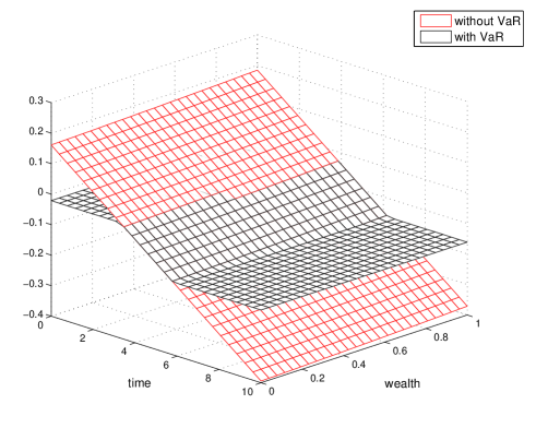
where N=N1(1p)/τ=37.74𝑁superscript𝑁11𝑝𝜏37.74N=N^{-1}(1-p)/\sqrt{\tau}=37.74, M=α+VaR¯/τ=5.273𝑀𝛼¯𝑉𝑎𝑅𝜏5.273M=\alpha+\overline{VaR}/\tau=5.273. Therefore the optimal control has the expression fVaR=max{f2,min{f1,f}}superscriptsubscript𝑓𝑉𝑎𝑅subscript𝑓2subscript𝑓1superscript𝑓f_{VaR}^{*}=\max\{f_{2},\min\{f_{1},f^{*}\}\}. We show the optimal strategy without the VaR limit as well as the constrained one on (x,t)[0,1]×[0,10]𝑥𝑡01010(x,t)\in[0,1]\times[0,10] in the Figure 1 below.

Refer to caption
Figure 1: Optimal strategies in case 3

As shown in this figure, the VaR constraint actually gives an upper and a lower bound surface to the strategy surface. From the expression of (12), we know that f1,2subscript𝑓12f_{1,2} are independent of x𝑥x and t𝑡t, and strictly negative in this case. Therefore the bound surfaces are horizontal and below level zero, which actually constrain the behavior of short-selling.

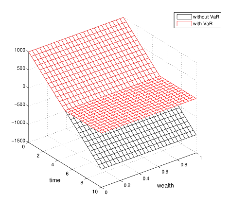
We could also compare the optimal value function with and without the VaR constraint, which are illustrated in Figure 2 for case 3. In both figures we could observe that the VaR constraint is active during the time period of approximately t[0,3][6,10]𝑡03610t\in[0,3]\cup[6,10]. The optimal function of constrained problem is identical to that of the unconstrained one during t[3,6]𝑡36t\in[3,6], and it becomes inferior when the constrain is active.
Refer to caption
Figure 2: Value functions in case 3

By changing the value of drift and diffusion parameter of the risky stock, investment in them becomes much more promising than in case 3. See the table below, note that we do not change the values of other parameters.

Table 2: Parameters
x𝑥x μ𝜇\mu σ𝜎\sigma α𝛼\alpha β𝛽\beta ρ𝜌\rho γ𝛾\gamma T𝑇T τ𝜏\tau p𝑝p VaR¯¯𝑉𝑎𝑅\overline{VaR}
1 0.8 0.02 0.01 0.14 0.2 1 10 1/260 0.01 0.02

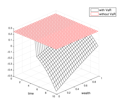
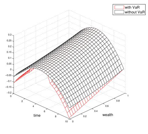
The setting of the parameters in Table 2 satisfies the condition of case 2, i.e. Nσ<μ𝑁𝜎𝜇N\sigma<\mu, where N=37.74𝑁37.74N=37.74. In Figure 3, we observe that when time t𝑡t is near 0, the investment in risky asset appears to be rather radical. This results from the superiority of the stock, and the investor can hardly get any loss under such circumstance, and therefore do not activate the VaR constraint. When time goes to approximately t=5𝑡5t=5, the constraint becomes active and gives the optimal strategy a lower bound near level zero, which is the only bound surface brought by the VaR constraint in case 2. The optimal value function surfaces are shown in Figure 4, where the surface of the constrained problem remains identical to that of the unconstrained problem until t=5𝑡5t=5. All as we expected, the constrained surface becomes inferior since then. Note that in this case, the optimal value without VaR constraint appears almost horizontal, which seems unreasonable. This results from the uncommon condition that N<μ/σ𝑁𝜇𝜎N<\mu/\sigma, which directly leads to the huge absolute value of B=0.5(μ/σ)2𝐵0.5superscript𝜇𝜎2B=-0.5(\mu/\sigma)^{2}. Look at the expressions of (16) and (17), the factor e2B(Tt)superscript𝑒2𝐵𝑇𝑡e^{2B(T-t)} almost annihilate the first three terms in V(t,x)𝑉𝑡𝑥V(t,x), which makes V(t,x)𝑉𝑡𝑥V(t,x) becomes a constant of 1/(4γ)14𝛾1/(4\gamma) approximately.

Refer to caption
Figure 3: Optimal strategies in case 2
Refer to caption
Figure 4: Value functions in case 2

References

  • Alexander and Baptista (2004) Alexander, G.J., Baptista, A.M., 2004. A comparison of VaR and CVaR constraints of portfolio selection with the mean-variance model. Management Science 50, 1261–1273.
  • Alexander and Baptista (2007) Alexander, G.J., Baptista, A.M., 2007. Mean-variance portfolio selection with ‘at-risk’ constraints and discrete distributions. Journal of Banking and Finance 31, 3761–3781.
  • Basak and Shapiro (2001) Basak, S., Shapiro, A., 2001. Value-at-risk-based risk management: Optimal policies and asset prices. Review of Financial Studies 14, 371–405.
  • Browne (1995) Browne, S., 1995. Optimal investment policies for a firm with a random risk process: exponential utility and minimizing the probability of ruin. Mathematics of Operation Research 20, 937–958.
  • Cox and Huang (1989) Cox, J.C., Huang, 1989. Optimal consumption and portfolio policies when asset prices follow a diffusion process. Journal of Economic Theory 49, 33–83.
  • Cuoco et al. (2008) Cuoco, D., He, H., Issaenko, S., 2008. Optimal dynamic trading strategies with risk limits. Operations Research 56, 358–368.
  • Duffie and Richardson (1991) Duffie, D., Richardson, H.R., 1991. Mean-variance hedging in continuous time. Annals of Applied Probability 1, 1–15.
  • Hakansson (1971) Hakansson, N.H., 1971. Multi-period mean-variance analysis: toward a general theory of portfolio choice. Journal of Finance 26, 857–884.
  • Jorion (1997) Jorion, P., 1997. Value at Risk: the New Benchmark for Controlling Market Risk. Irwin, Chicago, IL.
  • Karatzas et al. (1987) Karatzas, I., Lehoczky, J.P., Shreve, S.E., 1987. Optimal portfolio and consumption decisions for a small investor on a finite time-horizon. SIAM Journal on Control and Optimization 25, 1557–1586.
  • Kluppelberg and Korn (1998) Kluppelberg, C., Korn, R., 1998. Optimal portfolios with bounded value-at-risk. Working paper, Munich University of Technology.
  • Markowitz (1952) Markowitz, H., 1952. Portfolio selection. Journal of Finance 7, 77–91.
  • Markowitz (1959) Markowitz, H., 1959. Portfolio Selection: Efficient Diversification of Investment. New York: John Wiley & Sons.
  • Pirvu (2005) Pirvu, T.A., 2005. Maximizing portfolio growth rate under risk constraints. Doctoral Dissertation, Department of Mathematics, Carnegie Mellon University.
  • Pirvu (2007) Pirvu, T.A., 2007. Portfolio optimization under the value-at-risk constraint. Quantitative Finance 7, 125–136.
  • Pliska (1997) Pliska, S.R., 1997. Introduction to Mathematical Finance. Blackwell, Malden.
  • Samuelson (1969) Samuelson, P.A., 1969. Lifetime portfolio selection by dynamic stochastic programming. The Review of Economics and Statistics 51, 239–246.
  • Schweizer (1996) Schweizer, M., 1996. Approximation pricing and the variance-optimal martingale measure. The Annals of Probability 24, 206–236.
  • Yiu (2004) Yiu, K.F.C., 2004. Optimal portfolios under a value-at-risk contraint. Journal of Economic Dynamics and Control 28, 1317–1334.
  • Zhou and Li (2000) Zhou, X.Y., Li, D., 2000. Continuous-time mean-variance portfolio selection: a stochastic LQ framework. Applied Mathematics and Optimization 42, 19–33.