Nonlinear threshold Boolean automata networks and phase transitions

Abstract

In this report, we present a formal approach that addresses the problem of emergence of phase transitions in stochastic and attractive nonlinear threshold Boolean automata networks. Nonlinear networks considered are informally defined on the basis of classical stochastic threshold Boolean automata networks in which specific interaction potentials of neighbourhood coalition are taken into account. More precisely, specific nonlinear terms compose local transition functions that define locally the dynamics of such networks. Basing our study on nonlinear networks, we exhibit new results, from which we derive conditions of phase transitions.

${}^{1}\leavevmode\nobreak\$Université Joseph Fourier de Grenoble, TIMC-IMAG, AGIM, Faculté de médecine, 38700 La Tronche, France
${}^{2}\leavevmode\nobreak\$Université d’Évry – Val d’Essonne, IBISC, 91000 Évry, France
${}^{3}\leavevmode\nobreak\$Institut rhône-alpin des systèmes complexes, IXXI, 69007 Lyon, France

1 Introduction

The model of deterministic Threshold Boolean automata networks (called TBANs for short in the sequel) has been developped in the 1940’s by McCulloch and Pitts in [MP43] as a way to represent logically the interactions between neurons over time. In parallel [Ons44] has been addressed the problem of existence of phase transition in the two-dimensional Ising model of ferromagnetism [Isi25]. Taking into account that the classical Ising model can be generalised in the Boolean framework by the Boltzmann machine [AHS85], that is a stochastic variation around deterministic TBANs, we propose in this report a partial solution of the problem of emergence of phase transitions in this context, as it has been performed in the case of the classical Ising model by Dobrushin and Ruelle in [Dob68c, Rue69]. More precisely, we present a generalisation to nonlinear TBANs of theoretical results of phase transitions due to the influence of fixed boundary conditions already obtained in the framework of linear TBANs [DJS08, DS08].

After a presentation of important definitions for the study in Section 2, new theoretical results of phase transitions are given.

2 Model definitions

Although this work focuses on nonlinear TBANs whose architecture is partially defined in a part of the lattice on $\mathbb{Z}^{2}$, let us present TBANs from the general point of view. Let $N$ be such an arbitrary network. $N$ is composed by $n$ nodes interacting over time through a labelled digraph $G=(V,A)$, where $V$ is the set of nodes, elements of $\mathbb{Z}^{2}$, whose states are valued in $\{0,1\}$ ($0$ when the node is inactive and $1$ when it is active) and $A\subset V\times V$ is the set of arcs linking elements with each others. A TBAN is characterised by:

• an interaction matrix $W$ of order $n$: it defines the structure of $N$ and each coefficient $w_{i,j}\in\mathbb{R}$ is the label of arc $(j,i)$ of $A$ and gives the interaction weight node $j$ has on node $i$. If $w_{i,j}$ is null, then $(j,i)\notin A$, else node $j$ is said to be a neighbour of node $i$ and we note $j\in{\cal N}_{i}$. In this case, node $j$ is called an inducer/activator (resp. repressor/inhibitor) of node $i$ if $w_{i,j}>0$ (resp. $w_{i,j}<0$);

• a threshold vector $\Theta$ of dimension $n$: each element $\theta_{i}$ is called the activation threshold of node $i$.

• $n$ local transition functions which define the local evolution of each of the nodes in the TBANs. The general concept of the local evolution of a node $i$, namely the calculation of its state at time $t+1$ being given $N$ and the state of any node $k\in V$ at time $t$, is the following: if the potential of $i$ at time $t$, i.e., the sum of the interaction weights received from its active neighbours, is greater than (resp. not greater than) its activation threshold then its state at time $t+1$ equals $1$ (resp. $0$). Thus, if we denote by $x_{i}(t)$ the state of node $i$ at time $t$, the local transitions functions are:

  $$x_{i}(t+1)={\cal H}(\sum_{j\in{\cal N}_{i}}w_{i,j}\cdot x_{j}(t)-\theta_{i})\text{,}$$ (1)

  where ${\cal H}$ represents the Heaviside (or sign-step) function and is such that ${\cal H}(x)=\begin{cases}0&\text{if }x\leq 0\text{,}\\ 1&\text{otherwise.}\end{cases}$

An application $x:V\to\{0,1\}$ is called a configuration of $N$. In other words, the vector $x(t)=(x_{i}(t))_{i\in V}\in\{0,1\}^{n}$ is the configuration of $N$ at time $t$.

In the sequel, in order to highlight the emergence of phase transitions from the dynamical behaviour of TBANs, we will give a particular attention to the notion of boundary conditions. We will explain this later. Nevertheless, since we focus on TBANs on $\mathbb{Z}^{2}$, let us present general definitions of the notions of center and boundary of a graph $G=(V,A)$ that we will be able to adapt in the context of two-dimensional lattices. Basic notions of graph theory are considered to be known (cf. [Har69]).

Definition 1.

Let $G=(V,A)$ an arbitrary digraph. The boundary of $G$ is the set of its sources.

Let $u$ and $v$ be two distinct vertices of a digraph $G=(V,A)$. The distance $d(u,v)$ is the length of the shortest path linking $u$ to $v$. If there is no path from $u$ to $v$, $d(u,v)$ is defined as equal to $+\infty$.

Definition 2.

Let $G=(V,A)$ an arbitrary digraph. The eccentricity $\varepsilon(u)$ of a non isolated vertex $u\in V$ is the maximal distance less than $+\infty$ from $u$ and every other vertex of $G$, such that $\varepsilon(u)=\text{Max}_{v\,\in\,S\setminus u}(d(u,v)<+\infty)$.

Definition 3.

Let $G=(V,A)$ an arbitrary digraph. The centre of $G$ is the set of its vertices of minimal eccentricity.

In this report, we differentiate the notions of neighbourhood and strict neighbourhood of nonlinear two-dimentional TBANs according to the following definitions.

Definition 4.

Let $N$ be a two-dimensional TBAN on $\mathbb{Z}^{2}$. The neighbourhood ${\cal N}_{i}$ of node $i$ is the set composed of nearest-neighbours nodes (i.e., nodes at distance $1$ to $i$) of $i$ and $i$ itself.

Definition 5.

Let $N$ be a two-dimensional TBAN on $\mathbb{Z}^{2}$. The strict neighbourhood $\Lambda_{i}$ of node $i$ is such that $\Lambda_{i}={\cal N}_{i}\setminus\{i\}$.

Let us now define the properties of isotropy and translation invariance of the two-dimensional TBANs considered.

Definition 6.

Let $N$ be a two-dimensional TBAN on $\mathbb{Z}^{2}$. $N$ is isotropic if and only if:

$$\forall i\in N,\,\forall j,j^{\prime}\in{\cal N}_{i},\,w_{i,j}=w_{i,j^{\prime}}\text{.}$$

Definition 7.

Let $N$ be a two-dimensional TBAN on $\mathbb{Z}^{2}$. $N$ is translation invariant if and only if, given $j_{1},\ldots,j_{k}\in{\cal N}_{i}$, it holds that:

$$\forall i,i^{\prime}\in N,\,\exists s\in\mathbb{Z}^{d},\,i^{\prime}=i+s,\,\forall\ell\in\{1,\ldots,k\},\,j^{\prime}_{\ell}=j_{\ell}+s:\>w_{i,j_{\ell}}=w_{i^{\prime},j^{\prime}_{\ell}}\text{.}$$

As a consequence, TBANs considered in this study are symmetric, i.e., they are such that $\forall i,\forall j\in{\cal N}_{i},w_{i,j}=w_{j,i}$. According to these properties of isotropy and translation invariance, it is easy to see that Definition 3 can be applied directly to nonlinear TBANs on $\mathbb{Z}^{2}$. Conversely, the set of boundary obtained from the application of Definition 1 in this networks is the emptyset. Hence, boundary need to be built. The building process chosen consists in adding structurally specific nodes [Mar94]. This leads to the following definitions, considering an arbitrary TBANs $N$ whose underlying digraph $G=(V,A)$ is such that $V\subset\mathbb{Z}^{2}$ and that $V^{c}=\mathbb{Z}^{2}\setminus V$ is the set of vertices of $N^{c}$, said to be the complement of $N$ in $\mathbb{Z}^{2}$.

Definition 8.

The external boundary (called boundary for short), denoted by $\partial_{\mathrm{ext}}N$, is the set of nodes of $N^{c}$ at distance $1$ (in terms of distance in $\mathbb{Z}^{2}$) to at least one node of $N$ such that:

$$\partial_{\mathrm{ext}}N=\{i\in N^{c}\;|\;\exists j\in N:i\in{\cal N}_{j},j\notin{\cal N}_{i}\}\text{.}$$

An illustration of centre and boundary of a TBAN on $\mathbb{Z}^{2}$ is given in Figure 1.

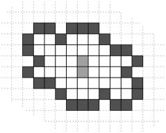
Figure 1: An arbitrary TBAN $N$ on $\mathbb{Z}^{2}$ whose nodes are in white and light grey (in the case of central nodes) and boundary $\partial_{\mathrm{ext}}N$ is the set of nodes coloured in dark grey.

TBANs in the sequel are attractive, i.e., they are such that $w_{i,i}<0$ and $\forall j\in\Lambda_{i},j\neq i,w_{i,j}>0$. Note also that activation thresholds are all fixed to $0$ and that auto-interaction potentials are always taken into account. Thus, the $w_{i,i}$’s play the role of activation thresholds. Furthermore, as said in the introduction, nonlinearity is added in the model of TBANs considering that interaction potentials that act on a node $i$ at time $t$ are not only reduced to the combination of the auto-interaction potential $w_{i,i}$ and the nearest-neighbours potential $\sum_{j\in\Lambda_{i}}w_{i,j}\cdot x_{j}(t)$. Indeed, we consider also coalition potentials. For instance, given a node $i$ of a TBAN $N$ at time $t$ whose state is not known, if we consider that the evolution of node $i$ takes into account coalition of neighbours couples, the interaction potential of node $i$ equals $w_{i,i}+\sum_{j\in\Lambda_{i}}w_{i,j}\cdot x_{j}(t)+\sum_{j,\ell\in{\cal N}_{i}}w_{i,\langle j,\ell\rangle}\cdot x_{j}(t)\cdot x_{\ell}(t)$, where $w_{i,\langle j,\ell\rangle}$ defines the interaction weight that the couple of active nodes $j$ and $\ell$ has on $i$. Remark that the $w_{i,i}$’s correspond to thresholds (considering them separately) and that the $i$’s play the role of elements of coalitions (considering them as parts of couples, triples, quadruples and quintuples in the sequel)

Let $T\in\mathbb{R^{+}}$ be the temperature parameter. We give the following notations of interaction potentials for every node $i$ of an arbitrary TBAN $N$ to ease the reading:

• $u_{0,i}=\frac{w_{i,i}}{T}$, called singleton potential, a function of the auto-interaction weight of an arbitrary node $i$ (always taken into account);

• $u_{1,i,j}=\frac{w_{i,j}}{T}$, where $j\,\in\,\Lambda_{i}$, couple potential, a function of interaction weights received by node $i$ from its strict nearest neighbours;

• $u_{2,i,\langle j,\ell\rangle}=\frac{w_{i,\langle j,\ell\rangle}}{T}$, where $j,\ell\,\in\,{\cal N}_{i}\;;\;j\neq\ell$, called triple potential, a function of interaction weights received by node $i$ from couples of its active neighbours;

• $u_{3,i,\langle j,\ell,m\rangle}=\frac{w_{i,\langle j,\ell,m\rangle}}{T}$, where $j,\ell,m\,\in\,{\cal N}_{i}\;;\;j\neq\ell\neq m$, called quadruple potential, a function of interaction weights received by node $i$ from triples of its active neighbours;

• $u_{4,i,\langle j,\ell,m,p\rangle}=\frac{w_{i,\langle j,\ell,m,p\rangle}}{T}$, where $j,\ell,m,p\,\in\,{\cal N}_{i}\;;\;j\neq\ell\neq m\neq p$, called quintuple potential, a function of interaction weights received by node $i$ from quadruples of its active neighbours.

Definition 9.

A stochastic TBAN $N$ of order $k$ on $\mathbb{Z}^{2}$ is a TBAN whose local transition function $f_{i}$ calculates the probability for node $i$ to be at state $1$ at time $t+1$ knowing the configuration projected on its neighbourhood ${\cal N}_{i}$ at time $t$ and taking into account $1$-uple, $2$-uple, …, $k$-uple potentials, with $2\leq k\leq 5$ such that:

$$\forall i\in N=\{1,\ldots,n\},P(x_{i}(t+1)=\alpha)=\frac{e^{\alpha\cdot(u_{0,i}+\sum_{j\in\Lambda_{i}}u_{1,i,j}\cdot x_{j}(t)+\phi_{i}^{k}(\Lambda_{i}))}}{1+e^{u_{0,i}+\sum_{j\in\Lambda_{i}}u_{1,i,j}\cdot x_{j}(t)+\phi_{i}^{k}(\Lambda_{i})}}\mathrm{,}$$ (2)

where $\phi_{i}^{k}(\Lambda_{i})$ is the nonlinear term such that:

$$\phi_{i}^{k}(\Lambda_{i})=\sum_{\stackrel{{\scriptstyle\stackrel{{\scriptstyle j,\ell,m,p,q\in{\cal N}_{i}}}{{j\neq\ell\neq m\neq p\neq q}}}}{{}}}u_{2,i,\langle j,\ell\rangle}\cdot x_{j}(t)\cdot x_{\ell}(t)+\ldots+\\ u_{k-1,i,\langle j,\ell,m,p,q\rangle}\cdot x_{j}(t)\cdot x_{\ell}(t)\cdot x_{m}(t)\cdot x_{p}(t)\cdot x_{q}(t)\mathrm{.}$$

Remark that, in the case of TBANs of order $2$ (i.e. $\phi_{i}^{k}(\Lambda_{i})=0$), if $T$ tends to $0$, then the stochastic local transitions functions defined in 2 are equivalent to the deterministic one defined in Equation 1. Before going further, let us insist that, from Definition 9, we derive that nonlinear TBANs studied in this report are stochastic TBANs of order at least equal to $3$.

3 Theoretical approach and phase transitions

Let us recall that TBANs considered in the sequel are isotropic, translation invariant, nonlinear. Moreover, we add that they are attractive. Given a stochastic TBAN $N$, that means that $\forall i\in N,\,u_{0,i}<0\;;\;\forall j\in\Lambda_{i},\,u_{1,i,j}>0$.

3.1 Projectivity matrix

Definition 10.

A cylinder $[A,B]$ is a configuration x such that:

$$[A,B]=\{x\;|\;\forall i\in A,\,x_{i}=1;\;\forall i\in B,\,x_{i}=0\}\text{.}$$

If $\mu$ denotes the invariant measure of a stochastic TBAN $N$ composed of $n$ nodes, indexed from $1$ to $n$, such that $n$ tends to infinity, we have the following projectivity and conditional relations. Indeed, we can write projectivity equations such that:

$$\forall A,B\subset N\;|\;A\cap B=\emptyset,\,\forall i\in A,\\ \mu([A,B])+\mu([A\setminus\{i\},B\cup\{i\}])=\mu([A\setminus\{i\},B])\text{,}$$

where $\mu([A,B])$ is the probability to observe the configuration $[A,B]$. We calso write conditional equations (i.e., the Bayes formulas) such that:

$$\forall i\in N,\,\mu([\{i\},\emptyset])=\sum_{A,B\subset N\;|\;A\cap B=\emptyset,\,A\cup B=N\setminus\{i\}}\Phi_{i}(A,B)\cdot\mu([A,B])\text{,}$$ (3)

where $\Phi_{i}(A,B)$ denotes the conditional probability that state of node $i$ equals $1$ knowing cylinder $[A,B]$ such that:

$$\mu(x_{i}=1\;|\;[A,B])=\Phi_{i}(A,B)=\frac{e^{u_{0,i}+\sum_{j\in\Lambda_{i}}u_{1,i,j}\cdot x_{j}(t)+\phi_{i}^{k}(\Lambda_{i}))}}{1+e^{u_{0,i}+\sum_{j\in\Lambda_{i}}u_{1,i,j}\cdot x_{j}(t)+\phi_{i}^{k}(\Lambda_{i})}}\text{.}$$

Consider $L=(N\cup\partial_{\text{ext}}N)\setminus\{O\}$ such that nodes of $L$ are ordered according to the lexical order of their indices. For every subset $K$ of $L$ of size $k$, we denote by $j_{K}$ the minimal index of nodes belonging to $K$. Projectivity matrix $M$ of order $2^{|L|}$ is defined such that (i) the $2^{|L|}-1$ first lines contain respectively the coefficients of the projectivity equations for any of the $2^{|L|}-1$ different couple $[L,K]$ and (ii) the last line contains the coefficients of the conditional equation $\mu([\{O\},\emptyset])=\sum_{A,B\subset N\leavevmode\nobreak\ |\leavevmode\nobreak\ A\cap B=\emptyset,A\cup B=N\setminus\{O\}}\Phi(A,B)\cdot\mu([A,B])$ that calculates the global probability for the central node to be active. The system of equations obtained from the projectivity and conditional equations is:

$$M\cdot\begin{pmatrix}\mu([L,\emptyset])\\ \mu([L\setminus\{1\},\{1\}])\\ \mu([L\setminus\{2\},\{2\}])\\ \vdots\\ \mu([K,L\setminus K])\\ \mu([K\setminus\{j_{K}\},(L\setminus K)\cup\{j_{K}\}])\\ \vdots\\ \mu([\{1\},L\setminus\{1\}])\\ \mu([\emptyset,L])\\ \end{pmatrix}=\begin{pmatrix}\mu([L\setminus\{1\},\emptyset])\\ \mu([L\setminus\{2\},\emptyset])\\ \ldots\\ \vdots\\ \mu([K\setminus\{j_{K}\},L\setminus K])\\ \ldots\\ \vdots\\ \mu([\emptyset,L\setminus\{1\}])\\ \mu([\{O\},\emptyset])\\ \end{pmatrix}\text{.}$$ (4)

From this system of equations, it is easy to write:

$$M=\begin{pmatrix}1&1&0&0&0&0&\ldots&0&0&0\\ 1&0&1&0&0&0&\ldots&0&0&0\\ 1&0&0&1&0&0&\ldots&0&0&0\\ 1&0&0&0&1&0&\ldots&0&0&0\\ 0&1&0&0&0&1&\ldots&0&0&0\\ \vdots&\vdots&\vdots&\vdots&\vdots&\vdots&\ddots&\vdots&\vdots&\vdots\\ 0&0&0&0&0&0&\ldots&0&1&0\\ 0&0&0&0&0&0&\ldots&0&0&1\\ \Phi_{0}&\Phi_{1}&\Phi_{2}&\Phi_{3}&\Phi_{4}&\Phi_{5}&\ldots&\Phi_{13}&\Phi_{14}&\Phi_{15}\end{pmatrix}\text{,}$$

where $\Phi_{0}=\Phi(\Lambda_{O},\emptyset)$, $\Phi_{1}=\Phi(\Lambda_{O}\setminus\{1\},\{1\})$, $\Phi_{2}=\Phi(\Lambda_{O}\setminus\{2\},\{2\})$, …, $\Phi_{5}=\Phi(\Lambda_{O}\setminus\{1,2\},\{1,2\})$, …, $\Phi_{13}=\Phi(\Lambda_{O}\setminus\{1,3,4\},\{1,3,4\})$, …and $\Phi_{15}=\Phi(\emptyset,\Lambda_{O})$..

Projectivity and conditional equations are in general linearly independent. However, under specific parametric conditions such as conditions of non uniqueness of the invariant measure, that is not the case. From the work of Dobrushin in [Dob68b, Dob68a, Dob68c, Dob69] in the framework of random fields, we derive the following definition.

Definition 11.

Let $N$ be an arbitrary stochastic attractive TBAN. Let $\partial_{\mathrm{ext}}^{0}N$ (resp. $\partial_{\mathrm{ext}}^{1}N$) be a boundary of $N$ composed of nodes whose state is fixed to $0$ (resp. $1$). The dynamical behaviour of $N$ admits a phase transition if and only if the invariant measure of the Markov chain associated to $N\cup\partial_{\mathrm{ext}}^{0}N$ does not equals that of the Markov chain associated to $N\cup\partial_{\mathrm{ext}}^{1}N$.

From Equations 4 and Definition 11, we can directly write the following proposition.

Proposition 1.

Given $N$ a stochastic attractive TBAN, the nullity of the determinant of its associated projectivity matrix $M$ is a necessary condition for $N$ to admit a phase transition in its dynamical behaviour.

Lemma 1.

[Dem81] The nullity of the determinant of a projectivity matrix is characterised by:

$$\text{\emph{Det}}M=0\iff\sum_{K\subset L}(-1)^{|L\setminus K|}\cdot\Phi(K,L\setminus K)=0\text{.}$$

Because of our hypotheses of isotropy and translation invariance, it is interesting to note that we can use the spatial Markovian property in order to make easier solving the system of projectivity equations. The spatial Markovian property implies that the state of the centre $O$ of a network $N$ depends only on the states of its neighbours, which allows to reduce $L$ to the centre $O$ strict neighbourhood, namely $\Lambda_{O}={\cal N}_{O}\setminus\{O\}$. Then, it is simpler to build the associated projectivity matrix $M_{O}$ of order $2^{2\cdot d}$.

3.2 Results

Basing our approach on Proposition 1, in this section, we prove the existence of parametric conditions of stochastic nonlinear TBANs that admit phase transitions.

First, from the spatial Markovian property of TBANs and because $|\Lambda_{O}|=0\mod 2$, the right member of the equation of Lemma 1 can be written pairing the subsets $K$ and $\Lambda_{O}\setminus K$, namely considering that:

$$(-1)^{|\Lambda_{O}\setminus K|}\cdot\Phi(K,\Lambda_{O}\setminus K)+(-1)^{|K|}\cdot\Phi(\Lambda_{O}\setminus K,K)\\ =(-1)^{|K|}[\Phi(K,\Lambda_{O}\setminus K)+\Phi(\Lambda_{O}\setminus K,K)]\text{.}$$

By hypothesis, nonlinear term $\phi_{O}^{k}(K)$ is symmetric and equals $-2\cdot u_{0,O}-\sum_{j\in\Lambda_{O}}u_{1,O,j}-\phi_{O}^{k}(\Lambda_{O}\setminus K)$. The symmetry property of the nonlinear term means that $\phi_{O}^{k}(K)=\phi_{O}^{k}(\Lambda_{O})-\phi_{O}^{k}(\Lambda_{O}\setminus K)$.

Lemma 2.

Given $N$ a nonlinear TBAN of order $k$ and $\phi_{O}^{k}(K)=-2\cdot u_{0,O}-\sum_{j\in\Lambda_{O}}u_{1,O,j}-\phi_{O}^{k}(\Lambda_{O}\setminus K)$ a symmetric nonlinear term such that $\phi_{O}^{k}(K)=\phi_{O}^{k}(\Lambda_{O})-\phi_{O}^{k}(\Lambda_{O}\setminus K)$, we have:

$$\phi_{O}^{k}(K)=\phi_{O}^{k}(\Lambda_{O})-\phi_{O}^{k}(\Lambda_{O}\setminus K)\iff\\ u_{0,O}+\frac{\sum_{j\in\Lambda_{O}}u_{1,O,j}}{2}+\frac{\phi_{O}^{k}(\Lambda_{O})}{2}=0\text{.}$$ (5)

Proof.

Let us note $\phi_{O}^{k}(\Lambda_{O})-\phi_{O}^{k}(\Lambda_{O}\setminus K)=\phi_{\text{sym}}$. Trivially, developing the left member of Equation 5 by definition of nonlinear terms, we can write:

$$\begin{split}\phi_{O}^{k}(K)=\phi_{\text{sym}}\iff\>&-2\cdot u_{0,O}-\sum_{j\in\Lambda_{O}}u_{1,O,j}-\phi_{O}^{k}(\Lambda_{O}\setminus K)=\phi_{\text{sym}}\\ \iff\>&-2\cdot u_{0,O}-\sum_{j\in\Lambda_{O}}u_{1,O,j}=\phi_{O}^{k}(\Lambda_{O})\\ \iff\>&-2\cdot u_{0,O}-\sum_{j\in\Lambda_{O}}u_{1,O,j}-\phi_{O}^{k}(\Lambda_{O})=0\\ \iff\>&-u_{0,O}-\frac{\sum_{j\in\Lambda_{O}}u_{1,O,j}}{2}-\frac{\phi_{O}^{k}(\Lambda_{O})}{2}=0\\ \iff\>&u_{0,O}+\frac{\sum_{j\in\Lambda_{O}}u_{1,O,j}}{2}+\frac{\phi_{O}^{k}(\Lambda_{O})}{2}=0\text{,}\end{split}$$

which is the expected result.   ∎

Lemma 3.

Let $N$ be a nonlinear TBAN of order $k$ and $\phi_{O}^{k}(\Lambda_{O})=-2\cdot u_{0,O}-\sum_{j\in\Lambda_{O}}u_{1,O,j}$ be the nonlinear term of $N$ when every nearest neighbour of its central node $O$ is active. Then:

$$u_{0,O}+\sum_{j\in\Lambda_{O}}\frac{u_{1,O,j}}{2}+\frac{\phi_{O}^{k}(\Lambda_{O})}{2}=0\iff\Phi(K,\Lambda_{O}\setminus K)+\Phi(\Lambda_{O}\setminus K,K)=1\text{.}$$

Proof.

First, let us show that $\Phi(K,\Lambda_{O}\setminus K)+\Phi(\Lambda_{O}\setminus K,K)=1$. It suffices to multiply $\Phi(K,\Lambda_{O}\setminus K)$ by $1=\frac{e^{-2\cdot u_{0,O}-\sum_{j\in\Lambda_{O}}u_{1,O,j}-\phi_{O}^{k}(\Lambda_{O})}}{e^{-2\cdot u_{0,O}-\sum_{j\in\Lambda_{O}}u_{1,O,j}-\phi_{O}^{k}(\Lambda_{O})}}$:

$$\Phi(K,\Lambda_{O}\setminus K)=\frac{e^{u_{0,O}+\sum_{j\in K}u_{1,O,j}+\phi_{O}^{k}(K)}}{1+e^{u_{0,O}+\sum_{j\in K}u_{1,O,j}+\phi_{O}^{k}(K)}}\times\frac{e^{-2\cdot u_{0,O}-\sum_{j\in\Lambda_{O}}u_{1,O,j}-\phi_{O}^{k}(\Lambda_{O})}}{e^{-2\cdot u_{0,O}-\sum_{j\in\Lambda_{O}}u_{1,O,j}-\phi_{O}^{k}(\Lambda_{O})}}\text{.}$$

Given $\delta$ defined by:

$$\delta=e^{-2\cdot u_{0,O}-\sum_{j\in\Lambda_{O}}u_{1,O,j}-\phi_{O}^{k}(\Lambda_{O})}+e^{-u_{0,O}-\sum_{j\in\Lambda_{O}\setminus K}u_{1,O,j}+\phi_{O}^{k}(K)-\phi_{O}^{k}(\Lambda_{O})}\text{,}$$

we have:

$$\Phi(K,\Lambda_{O}\setminus K)=\frac{e^{-u_{0,O}-\sum_{j\in\Lambda_{O}\setminus K}u_{1,O,j}+\phi_{O}^{k}(K)-\phi_{O}^{k}(\Lambda_{O})}}{\delta}\text{.}$$

By hypothesis, $\phi_{O}^{k}(\Lambda_{O})=-2\cdot u_{0,O}-\sum_{j\in\Lambda_{O}}u_{1,O,j}$. As a consequence, we have $e^{-2\cdot u_{0,O}-\sum_{j\in\Lambda_{O}}u_{1,O,j}-\phi_{O}^{k}(\Lambda)}=1$. Moreover, given that nonlinear term $\phi_{O}^{k}$ is symmetric:

$$\begin{split}\Phi(K,\Lambda_{O}\setminus K)&=\frac{e^{-u_{0,O}-\sum_{j\in\Lambda_{O}\setminus K}u_{1,O,j}-\phi_{O}^{k}(\Lambda_{O}\setminus K)}}{1+e^{-u_{0,O}-\sum_{j\in\Lambda_{O}\setminus K}u_{1,O,j}-\phi_{O}^{k}(\Lambda_{O}\setminus K)}}\\ &=1-\frac{e^{u_{0,O}+\sum_{j\in\Lambda_{O}\setminus K}u_{1,O,j}+\phi_{O}^{k}(\Lambda_{O}\setminus K)}}{1+e^{u_{0,O}+\sum_{j\in\Lambda_{O}\setminus K}u_{1,O,j}+\phi_{O}^{k}(\Lambda_{O}\setminus K)}}\\ &=1-\Phi(\Lambda_{O}\setminus K,K)\text{.}\end{split}$$

So, we can write:

$$\Phi(K,\Lambda_{O}\setminus K)+\Phi(\Lambda_{O}\setminus K,K)=1\iff\Phi(\Lambda_{O}\setminus K,K)=1-\Phi(K,\Lambda_{O}\setminus K)\text{.}$$

Expanding left and right members of the equation above leads to:

$$\frac{e^{u_{0,O}+\sum_{j\in\Lambda_{O}\setminus K}u_{1,O,j}+\phi_{O}^{k}(\Lambda_{O}\setminus K)}}{1+e^{u_{0,O}+\sum_{j\in\Lambda_{O}\setminus K}u_{1,O,j}+\phi_{O}^{k}(\Lambda_{O}\setminus K)}}=1-\frac{e^{u_{0,O}+\sum_{j\in K}u_{1,O,j}+\phi_{O}^{k}(K)}}{1+e^{u_{0,O}+\sum_{j\in K}u_{1,O,j}+\phi_{O}^{k}(K)}}\text{,}$$

which is equivalent to:

$$\frac{e^{u_{0,O}+\sum_{j\in\Lambda_{O}\setminus K}u_{1,O,j}+\phi_{O}^{k}(\Lambda_{O}\setminus K)}}{1+e^{u_{0,O}+\sum_{j\in\Lambda_{O}\setminus K}u_{1,O,j}+\phi_{O}^{k}(\Lambda_{O}\setminus K)}}=\frac{e^{-u_{0,O}-\sum_{j\in K}u_{1,O,j}-\phi_{O}^{k}(K)}}{1+e^{-u_{0,O}-\sum_{j\in K}u_{1,O,j}-\phi_{O}^{k}(K)}}\text{.}$$

Let us proceed to the following change of variables: let $\delta_{1}$ (resp. $\delta_{2}$) be the denominator of the left member (resp. of the right member) and $\eta_{1}$ (resp. $\eta_{2}$) the numerator of the left member (resp. of the right member) of the equation above. We have then:

$$\begin{split}\frac{\eta_{1}}{\delta_{1}}=\frac{\eta_{2}}{\delta_{2}}&\iff\frac{\eta_{1}\cdot\delta_{2}}{\delta_{1}\cdot\delta_{2}}=\frac{\eta_{2}\cdot\delta_{1}}{\delta_{2}\cdot\delta_{1}}\\ &\iff\eta_{1}\cdot\delta_{2}=\eta_{2}\cdot\delta_{1}\text{.}\end{split}$$

Let $\zeta$ be such that:

$$\zeta=e^{\sum_{j\in\Lambda_{O}\setminus K}u_{1,O,j}-\sum_{j\in K}u_{1,O,j}+\phi_{O}^{k}(\Lambda_{O}\setminus K)-\phi_{O}^{k}(K)}\text{.}$$

We have:

$$\begin{split}\frac{\eta_{1}}{\delta_{1}}=\frac{\eta_{2}}{\delta_{2}}&\iff\eta_{1}+\zeta=\eta_{2}+\zeta\\ &\iff\eta_{1}=\eta_{2}\text{.}\end{split}$$

Thus, we can write:

$$\frac{\eta_{1}}{\delta_{1}}=\frac{\eta_{2}}{\delta_{2}}\iff e^{u_{0,O}+\sum_{j\in\Lambda_{O}\setminus K}u_{1,O,j}+\phi_{O}^{k}(\Lambda_{O}\setminus K)}=e^{-u_{0,O}-\sum_{j\in K}u_{1,O,j}-\phi_{O}^{k}(K)}\\ \iff u_{0,O}+\sum_{j\in\Lambda_{O}\setminus K}u_{1,O,j}+\phi_{O}^{k}(\Lambda_{O}\setminus K)=-u_{0,O}-\sum_{j\in K}u_{1,O,j}-\phi_{O}^{k}(K)\\ \iff\phi_{O}^{k}(K)=-2\cdot u_{0,O}-\sum_{j\in\Lambda_{O}\setminus K}u_{1,O,j}-\sum_{j\in K}u_{1,O,j}-\phi_{O}^{k}(\Lambda_{O}\setminus K)\text{.}$$

And, thus, we have:

$$\frac{\eta_{1}}{\delta_{1}}=\frac{\eta_{2}}{\delta_{2}}\iff\phi_{O}^{k}(K)=-2\cdot u_{0,O}-\sum_{j\in\Lambda_{O}}u_{1,O,j}-\phi_{O}^{k}(\Lambda_{O}\setminus K)\text{.}$$

Hence, by hypothesis:

$$\begin{split}\frac{\eta_{1}}{\delta_{1}}=\frac{\eta_{2}}{\delta_{2}}&\iff\phi_{O}^{k}(K)=\phi_{O}^{k}(\Lambda_{O})-\phi_{O}^{k}(\Lambda_{O}\setminus K)\text{,}\\ \end{split}$$

which is the expected result.   ∎

From Lemmas 2 and 3, it is easy to derive the following theorem that highlights an empirical sufficient condition of phase transitions in nonlinear TBANs of order $k$ on $\mathbb{Z}^{d}$.

Theorem 1.

Let $N$ be a nonlinear TBAN of order $k$. We have:

$$\phi_{O}^{k}(K)=\phi_{O}^{k}(\Lambda_{O})-\phi_{O}^{k}(\Lambda_{O}\setminus K)\implies\text{Det}M=0\text{,}$$

which means that the symmetry property of the non linear term is an empirical sufficient condition for detM to vanish, allowing consequently phase transitions to occur.

Proof.

From Lemma 1 and because of the parity of the cardinal of $\Lambda_{O}$, we can write:

$$\begin{split}\text{\emph{Det}}M=0\iff\>&\sum_{K\subset\Lambda_{O}}(-1)^{|\Lambda_{O}\setminus K|}\cdot\Phi(K,L\setminus K)=0\\ \iff\>&\sum_{K\subset\Lambda_{O}}(-1)^{|\Lambda_{O}\setminus K|}\times\frac{[\Phi(K,L\setminus K)+\Phi(L\setminus K,K)]}{2}=0\text{.}\end{split}$$

Then Lemma 3 leads to:

$$\begin{split}\text{\emph{Det}}M=0&\iff\sum_{K\subset\Lambda_{O}}(-1)^{|\Lambda_{O}\setminus K|}\cdot\frac{1}{2}=0\text{,}\\ \end{split}$$

which is always true. As a result, since Lemmas 2 and 3 are based on the hypothesis of symmetry of the non linear term, we have from Lemma 1:

$$u_{0,O}+\frac{\sum_{j\in\Lambda_{O}}u_{1,O,j}}{2}+\frac{\phi_{O}^{k}(\Lambda_{O})}{2}=0\implies\text{\emph{Det}}M=0\text{,}$$

which is the expected result.   ∎

References

- [AHS85] D. H. Ackley, G. E. Hinton, and T. J. Sejnowski. A learning algorithm for Boltzmann machines. Cognitive Science, 9:147–169, 1985.
- [Dem81] J. Demongeot. Asymptotic inference for Markov random field on . Springer Series in Synergetics, 9:254–267, 1981.
- [DJS08] J. Demongeot, C. Jézéquel, and S. Sené. Boundary conditions and phase transitions in neural networks. Theoretical results. Neural Networks, 21(7):971–979, 2008.
- [Dob68a] R. L. Dobrushin. Gibbsian random fields for lattice systems with pairwise interactions. Functional Analysis and Its Applications, 2(4):292–301, 1968.
- [Dob68b] R. L. Dobrushin. The description of a random field by means of conditional probabilities and conditions of its regularity. Theory of Probability and its Applications, 13(2):197–224, 1968.
- [Dob68c] R. L. Dobrushin. The problem of uniqueness of a Gibbsian random field and the problem of phase transitions. Functional Analysis and Its Applications, 2(4):302–312, 1968.
- [Dob69] R. L. Dobrushin. Gibbsian random fields. The general case. Functional Analysis and Its Applications, 3(1):22–28, 1969.
- [DS08] J. Demongeot and S. Sené. Boundary conditions and phase transitions in neural networks. Simulation results. Neural Networks, 21(7):962–970, 2008.
- [Har69] F. Harary. Graph Theory. Addison-Wesley, 1969.
- [Isi25] E. Ising. Beitrag zur theorie des ferromagnetismus. Zeitschrift für Physics, 31(1):253–258, 1925.
- [Mar94] F. Martinelli. On the two-dimensional dynamical Ising model in the phase coexistence region. Journal of Statistical Physics, 76(5–6):1179–1246, 1994.
- [MP43] W. S. McCulloch and W. Pitts. A logical calculus of the ideas immanent in nervous activity. Bulletin of Mathematical Biophysics, 5(4):115–133, 1943.
- [Ons44] L. Onsager. Crystal statistics. I. A two-dimensional model with an order-disorder transition. Physical Review, 65:117–149, 1944.
- [Rue69] D. Ruelle. Statistical mechanics: rigourous results. W. A. Benjamin, 1969.