Dynamo action in thermally unstable interstellar flows

Abstract

Numerous studies have investigated the role of thermal instability in regulating the phase transition between the cold cloudy and warm diffuse medium of the interstellar medium. Considerable interest has also been devoted to investigating the properties of turbulence in thermally unstable flows, with a special emphasis on molecular clouds and the possibility of star formation. In this study, we investigate another setting in which this instability may be important, namely its effect on dynamo action in interstellar flows. The setup we consider is a three dimensional periodic cube of gas with an initially weak magnetic field, subject to heating and cooling, the properties of which are such that thermal instability is provoked in a certain temperature regime. Dynamo action is established through external forcing on the flow field. By comparing the results with a cooling function with exactly the same net effect but no thermally unstable regime, we find the following. Reference runs with non-helical forcing were observed to produce no small-scale dynamo action below the Reynolds number 97. Therefore, we expect the magnetic fields generated in the helical runs to be purely due to the action of a large-scale dynamo mechanism. The critical Reynolds number for the onset of the large-scale dynamo was observed to roughly double between the thermally stable versus unstable runs, the conclusion being that the thermal instability makes large-scale dynamo action more difficult. Whereas density and magnetic fields were observed to be almost completely uncorrelated in the thermally stable cases investigated, the action of thermal instability was observed to produce a positive correlation of the form $B\propto\rho^{0.2}$. This correlation is rather weak, and in addition it was observed to break down at the limit of highest densities.

1. Introduction

The role of thermal instability (hereafter TI) in regulating the phase transition between the cold and warm neutral components, normally denoted with CNM and WNM, of the interstellar matter (hereafter ISM) has been intensively studied over several decades (for a review, see e.g. Cox, 2005) since the original seminal paper by Field, Goldsmith, & Habing (1969) proposed this mechanism, known as the FGH-model. According to it, two thermally stable phases (cold and cloudy; warm and diffuse) co-exist in pressure equilibrium regulated by the presence of a thermally unstable phase at an intermediate temperature. Now it is observationally well-established that the picture is not quite simple as that, but there is also a third, hot and dilute, component of the ISM. The first model that incorporated the hot component, generated by the action of supernova explosions (hereafter SNe), to the FGH model was presented by McKee & Ostriker (1977). This model suggested rather drastic modifications to the structure of ISM: with the inclusion of SN-action, most (70–80 percent) of the gas became filled by the hot component. Since then, with extensive numerical modelling of the SN-driven flows (e.g. Chiang & Prendergast, 1985; Rosen et al., 1993; Korpi et al., 1999; Gazol-Patiño & Passot, 1999; de Avillez, 2000; Balsara et al., 2004; Gressel et al., 2008) and more careful observational determinations (for a review, see e.g. Ferrière, 2001), the estimates of the filling factor of the hot component have been reduced to 10–30 percent near the Galactic midplane, being bigger at larger heights. Moreover, most of the hot gas seems to be confined in large bubbles created by clustered SN activity rather than being distributed homogeneously around the Galaxy (e.g. Ferrière, 2001).

A number of investigations of interstellar turbulence at relevant scales for studying molecular cloud formation or any other process of interest in the atomic ISM still use the FGH-picture as a starting point. This seems justified in the light of the hot gas filling factor being relatively small near the Galactic midplane. Various numerical studies investigating the interaction of turbulence and TI have been published. In most of these studies turbulence is forced by sources other than the TI itself: random turbulent forcing at varying scales and Mach numbers (e.g. Gazol et al., 2005), localized injections of energy mimicking stellar winds (e.g. Vázquez-Semadeni et al., 2000), the magnetorotational instability (e.g. Piontek & Ostriker, 2007), and systematic large-scale motions such as propagating shock fronts (e.g. Koyama & Inutsuka, 2002) and converging flows e.g. by Audit & Hennebelle (2005), Heitsch et al. (2005) and Vázquez-Semadeni et al. (2006) have been considered. One of the major findings from these models is that, due to the turbulence present in the system, large pressure deviations are generated and significant amounts of gas can exist in the thermally unstable regime. These results suggest, as already noted by Norman & Ferrara (1996), that the FGH picture of the ISM exhibiting ’discrete’ temperatures and densities and a unique equilibrium pressure should be modified in the direction of a ’continuum’ of states with an overall pressure balance but with large deviations from it.

In recent years the possibility of driving turbulence by the TI itself has also received some attention. Contrary to Kritsuk & Norman (2002), who found turbulence to die out as a power law, Inutsuka & Koyama (2007) found the turbulence to be sustained—at least for times up to $0.1\,{\rm Gyr}$, although the turbulent motions were too weak to be significant in the ISM. However, in the study by Brandenburg, Korpi, & Mee (2007), hereafter BKM07, the TI-generated turbulence was observed to decay in simulations extending to more than $1\,{\rm Gyr}$. Even the inclusion of large-scale shear did not help sustain the turbulence. Therefore, it seems evident that TI alone cannot produce self-sustained turbulence, in contrast to the gravitational instability studied by Gammie (2001) or the magnetorotational turbulence studied e.g. by Hawley, Gammie, & Balbus (1995) and Brandenburg et al. (1995).

The line-of-sight magnetic field strengths in dense molecular clouds, as revealed by the Zeeman splitting measurements of molecular lines, follow an approximate correlation of the form $B_{||}\propto n(H_{2})^{1/2}$, where $n(H_{2})$ is the density of the molecular hydrogen in the cloud, e.g. Crutcher (1999) (for a recent review, see e.g. Heiles & Crutcher, 2005). For diffuse clouds at lower densities n $\sim$ 0.1 – 100 cm⁻³ also seen through the Zeeman splitting of the HI line, no clear correlation between the magnetic field strength and density has been found (Troland & Heiles, 1986; Myers, Goodman, Gusten, & Heiles, 1995; Heiles & Crutcher, 2005). Passot & Vázquez-Semadeni (2003) suggested that this phenomenon could be due to the strongly varying Alfvénic Mach number, $\rm Ma_{a}$, in the turbulent ISM. At low values of $\rm Ma_{a}$, their analysis revealed an anti-correlation between the density and magnetic pressure due to the dominance of slow MHD waves. At higher $\rm Ma_{a}$, both slow and fast modes were possible, their interference leading to de-correlation for intermediate densities, and re-correlation for the highest densities. Heitsch et al. (2004) proposed an alternative mechanism, namely ambipolar diffusion, enhanced by the vigorous interstellar turbulence to be rapid enough to de-correlate the magnetic field from the density. The fast reconnection of magnetic field lines in the cloudy medium has also been discussed in this context, e.g. by Santos-Lima et al. (2010).

In addition, there is observational evidence of it being particularly the regular component, seen through synchrotron emission, that is de-correlated from the gas density. For instance, observations of barred spiral galaxies indicate the magnetic fields forming coherent structures over the length scale of the bars themselves are not reacting as strongly as expected to the compression by the systematic motions occurring in the bars (e.g. NGC 1097 and NGC 1365 analyzed by Beck et al., 2005). A similar situation has been reported in M51 by Fletcher et al. (2010), where the regular magnetic field is not strongest at the locations of the highest compression due to the spiral density wave. It has been proposed that such a loose or completely nonexistent correlation between the regular component of the magnetic field and the diffuse clouds could be a result of the detachment of the large-scale field from the clouds in a fragmentation process such as the one resulting from thermal or gravitational instability (Beck et al., 2005).

During the recent years, numerical models in the magnetohydrodynamic regime including thermal and gravitational instabilities able to reach down to the size of the molecular clouds themselves have been developed by e.g. Hennebelle et al. (2008), Heitsch & Hartmann (2008) and Banerjee et al. (2009). The results from these calculations seem to be in very good agreement with the observations, i.e. producing very weak correlation between the magnetic field and density for lower densities, while re-establishing the correlation of the form $B\propto n^{1/2}$ at higher densities. Our first motivation in this manuscript is to isolate the role of thermal instability in the process that produces the density-magnetic field correlation.

Another interesting question that has not gained much attention is the effect of thermal instability on the galactic dynamo mechanism. Evidently, thermal instability cannot be expected by itself to drive turbulence that could generate and maintain a self-sustained dynamo. Rather, it can be expected to influence the dynamics of a flow that is dynamo active, and therefore may also have an effect on the properties of the dynamo. This is the second aspect we are aiming at investigating in detail in the present manuscript.

We adopt a very simple approach: as in our previous study of thermal instability under a purely hydrodynamic setting (BKM07), we use a cubic periodic computational domain filled with an initially uniform, non-stratified gas that has the characteristics of the atomic component of the interstellar matter. Unlike BKM07, a weak random magnetic field is inserted into the system at the initial state. Dynamo action is achieved by using an external forcing function on the flow field. In the case where the forcing is helical, a large-scale dynamo develops. For non-helical forcings, only small-scale dynamo action can be expected in our setting. The system is then subjected to either thermally stable or unstable cooling functions balanced by a constant UV-heating function. From the resulting set of models, we monitor the growth rate and saturation properties of the different types of dynamos, and the correlation between the density and magnetic field developing in each system.

2. Model

2.1. Governing equations

We consider the governing equations for a compressible and magnetized perfect gas,

$${{\rm D}{}\ln\rho\over{\rm D}{}t}=-\mbox{\boldmath$\nabla$}{}\cdot\mbox{\boldmath$u$}{},$$ (1)

$$\rho{{\rm D}{}\mbox{\boldmath$u$}{}\over{\rm D}{}t}=-\mbox{\boldmath$\nabla$}{}p+\mbox{\boldmath$J$}{}\times\mbox{\boldmath$B$}{}+\mbox{\boldmath$\nabla$}{}\cdot(2\nu\rho\mbox{\boldmath${\sf S}$}{})+\bm{f}_{\rm force},$$ (2)

$$T{{\rm D}{}s\over{\rm D}{}t}=2\nu\mbox{\boldmath${\sf S}$}{}^{2}+{1\over\rho}\mbox{\boldmath$\nabla$}{}\cdot\left(c_{p}\rho\chi\mbox{\boldmath$\nabla$}{}T\right)-{\cal L},$$ (3)

$${{\rm D}{}\mbox{\boldmath$A$}{}\over{\rm D}{}t}=-(\mbox{\boldmath$\nabla$}{}\mbox{\boldmath$u$}{})^{\rm T}\mbox{\boldmath$A$}{}-\mu_{0}\eta\mbox{\boldmath$J$}{},$$ (4)

where $u$ is the velocity, $\rho$ the density, $s$ the specific entropy, $A$ the vector potential of the magnetic field $\mbox{\boldmath$B$}{}=\mbox{\boldmath$\nabla$}{}\times\mbox{\boldmath$A$}{}$, $\mbox{\boldmath$J$}{}=\mu_{0}^{-1}\mbox{\boldmath$\nabla$}{}\times\mbox{\boldmath$B$}{}$ the current, with ${\sf S}_{ij}=\frac{1}{2}(u_{i,j}+u_{j,i})-\frac{1}{3}\delta_{ij}\mbox{\boldmath$\nabla$}{}\cdot\mbox{\boldmath$u$}{}$ being the traceless rate of strain tensor, $\nu$ is the kinematic viscosity, $\chi$ is the thermal diffusivity, $\eta$ the magnetic diffusivity, $\mu_{0}$ the permeability of free space, and ${\cal L}$ is the net cooling/heating, i.e. the difference between cooling and heating functions, with

$${\cal L}=\rho\Lambda-\Gamma,$$ (5)

where $\Gamma=\mbox{const}$ is assumed for the heating function; here we consider the photoelectric heating by interstellar grains caused by the stellar UV radiation field, for which Wolfire et al. (1995) give the value of $0.015\,{\rm erg}\,{\rm g}^{-1}\,{\rm s}^{-1}$ at $n=1\,{\rm cm}^{-3}$.

Following common practice, we adopt a perfect gas where $\rho$ and $s$ are related to pressure $p$ and temperature $T$ via the relations

$$p={{\cal R}\over\mu}\rho T,\quad s=c_{v}\ln p-c_{p}\ln\rho+s_{0},$$ (6)

where ${\cal R}=8.314\times 10^{7}\,{\rm cm}^{2}\,{\rm s}^{-2}\,{\rm K}^{-1}$ is the universal gas constant, and $\mu$ is the mean molecular weight; in this study we have adopted $\mu=0.62$ in all cases, corresponding to complete ionization. This is naturally unrealistic for the cold and cool phases, for which the ionization fraction can be expected to be low. To choose a higher mean molecular weight better corresponding to the cooler phases, however, would be equally unrealistic, as a significant fraction of the gas is still expected to be ionized. A better approach to deal with this issue would be to follow the ionization fraction and adjust $\mu$ accordingly. This, however, is out of the scope of the present study. The rest of the thermodynamic quantities read ${\cal R}/\mu=c_{p}-c_{v}$, with $c_{p}$ and $c_{v}$ being the specific heats at constant pressure and volume, respectively, $\gamma=c_{p}/c_{v}=5/3$ is their assumed ratio, $c_{\rm s}$ is the adiabatic sound speed, $T$ is the temperature, and the two are related to the other quantities via $c_{\rm s}^{2}=\gamma{\cal R}T/\mu$. The specific entropy is defined up to a constant $s_{0}$, the value of which is unimportant for the dynamics.

We adopt a parameterization of the cooling function equal to that given by Sánchez-Salcedo et al. (2002), which has been obtained by fitting a piecewise power law function of the form

$$\Lambda(T)=C_{i,i+1}T^{\beta_{i,i+1}}\quad\mbox{for $T_{i}\leq T<T_{i+1}$},$$ (7)

to the equilibrium pressure curve of the standard model of Wolfire et al. (1995) for the ISM in the solar neighborhood. This cooling function has a thermally unstable branch in between the temperatures $T=313$ K and $6102$ K, where $\beta<1$; henceforth, we denote this cooling function with ’SS’. To be able to extract the effect of the thermally unstable branch of the cooling function on the flow dynamics, we fabricate a thermally stable counterpart, denoted with ’TS’, with the criterion that for constant density, the net cooling caused by these two functions is the same. The coefficients for both cooling functions are given in Table LABEL:Tcooling, and a comparison plot is presented in Fig. 1. In this figure, we plot the heating-cooling equilibrium pressures with the two cooling functions, with respect to the chosen value of the UV-heating function $\Gamma$.

We consider the case where turbulence is driven by an additional body force, $\bm{f}_{\rm force}$, in the momentum equation. Following Käpylä & Brandenburg (2009), we use a forcing function $\bm{f}_{\rm force}$ given by

$$\bm{f}_{\rm force}(\bm{x},t)={\rm Re}\{N\bm{f}_{\bm{k}(t)}\exp[i\bm{k}(t)\cdot\bm{x}+i\phi(t)]\}\;,$$ (8)

where $\bm{x}$ is the position vector, $N=f_{0}c_{\rm s}(kc_{\rm s}/\delta t)^{1/2}$ is a normalization factor, $f_{0}$ is the forcing amplitude, $k=|\bm{k}|$ the wavevector, $\delta t$ is the length of the time step, and $-\pi<\phi(t)<\pi$ a random delta-correlated phase. The wavevector and the random phase change at every time step, resulting in a forcing function that is $\delta$-correlated in time. We force the system with transverse helical waves,

$$\bm{f}_{\bm{k}}={\sc R}\cdot\bm{f}_{\bm{k}}^{\rm nohel}\ \ {\rm with}\ \ {\sc R}_{ij}=\frac{\delta_{ij}-i\sigma\epsilon_{ijk}\hat{k}_{k}}{\sqrt{1+\sigma^{2}}}.$$ (9)

The helical case with positive helicity corresponds to $\sigma=1$, with the forcing function

$$\bm{f}_{\bm{k}}^{\rm nohel}=\left(\bm{k}\times\hat{\bm{e}}\right)/\sqrt{\bm{k}^{2}-\left(\bm{k}\cdot\hat{\bm{e}}\right)^{2}},$$ (10)

where $\hat{\bm{e}}$ is an arbitrary unit vector not aligned with the forcing wavevector.

Thus, $\bm{f}_{\bm{k}}$ can be chosen to give either non-helical ($\sigma=0$) or helical ($\sigma=1$) transversal waves with $|\bm{f}_{\bm{k}}|^{2}=1$, where ${\bm{k}}$ is chosen randomly from a predefined range in the vicinity of the average non-dimensional wavenumber $k_{\rm f}/k_{1}$ at each time step. Here $k_{1}$ is the wavenumber corresponding to the domain size, and $k_{\rm f}$ is the wavenumber of the energy-carrying scale, chosen to be between 2.5 and 3.5 times the smallest wavenumber in the box, $k_{1}=2\pi/(0.2\,{\rm kpc})$. In a system very similar to the one under study here, namely Brandenburg (2001), large-scale dynamo action was found with helical forcing. In the presence of shear, non-helical forcing has also been found to excite a large-scale dynamo (e.g. Yousef et al., 2008), but in the absence of it, can lead only to small-scale dynamo action (e.g. Haugen et al., 2004). In this study, both types of forcings are investigated, in the hope to study the effect of TI both on the small- and large-scale dynamos. We systematically vary the type and vigor of the forcing, and subject the gas either to thermally stable or unstable cooling function; the parameters for the runs produced can be found from Table 2.

Table 1Coefficients for the thermally unstable (SS) and stable (TS) cooling curves.

$i$ $T_{i}$ $C^{U}_{i,i+1}$ $\beta^{U}_{i,i+1}$ $C^{S}_{i,i+1}$ $\beta^{S}_{i,i+1}$ 1 10 $3.42\times 10^{16}$ 2.12 $2.16\times 10^{17}$ 1.50 2 141 $9.10\times 10^{18}$ 1.00 $2.56\times 10^{18}$ 1.00 3 313 $1.11\times 10^{20}$ 0.56 $2.56\times 10^{18}$ 1.00 4 6102 $2.00\times 10^{8}$ 3.67 $2.00\times 10^{8}$ 3.67 5 $10^{5}$ $7.96\times 10^{29}$ $-0.65$ $7.96\times 10^{29}$ $-0.65$

It is convenient to measure time in gigayears (Gyr), speed in km/s, and density in units of $10^{-24}\,{\rm g}\,{\rm cm}^{-3}$. The resulting unit of pressure is $10^{-14}\,{\rm dyn}$, and the unit of length $1(\,{\rm km/s})\times\,{\rm Gyr}\approx 1\,{\rm kpc}$. Viscosity and thermal diffusivity are measured in units of $\,{\rm Gyr}\,\,{\rm km}^{2}\,{\rm s}^{-2}$. The resulting unit for energy is $E_{0}$=3.2$\times 10^{50}$ ergs, and the unit of magnetic field is 0.35$\mu$G.

We use periodic boundary conditions in all three directions for a computational domain of size $(200\,{\rm pc})^{3}$. Near the galactic midplane, the cell size reported from SN-turbulence range in between 60-100 pc (e.g. Korpi et al., 1999); this can be thought as the relevant length scale for the galactic dynamo near the midplane, one of the basic ingredients of which SN-turbulence is thought to be (see e.g. Ferrière, 2001). Therefore, the chosen computational domain size can be thought of as a compromise in being large enough to contain a few turbulent SN cells but small enough to follow the phase segregation process into cold cloudy and warm dilute phases of the ISM.

We use the Pencil Code, which is a non-conservative, high-order, finite-difference code (sixth order in space and third order in time) for solving the compressible hydrodynamic equations. Because of the non-conservative nature of the code, diagnostics giving the total mass and total energy (accounting for heating/cooling terms) are monitored and simulations are only deemed useful if these quantities are in fact conserved to reasonable precision. The mesh spacings in the three directions are assumed to be the same, i.e. $\delta x=\delta y=\delta z$. In the simulations reported in this manuscript, the size of the computational grid is $128^{3}$, yielding a resolution of roughly 1.6 pc in our model. We note that a resolution study in a corresponding hydrodynamic setup was made in our previous study (BKM07), where doubling the resolution was observed to not significantly change the flow properties.

As in our previous study (BKM07), see also Koyama & Initsuka (2004) and Piontek & Ostriker (2005), we include thermal conduction, which stabilizes the gas at wavelengths larger than the critical one of the condensation mode (Field, 1965). This wavelength is usually referred to as the Field length, and is three orders of magnitude larger in our simplified model than in reality (of the order of 0.001pc). The required stabilizing effect could, in principle, be achieved by high enough numerical diffusion arising from the scheme itself (see e.g. Gazol et al., 2005), but with our high-order finite-difference scheme this effect is not large enough with the chosen viscosity coefficients. We emphasize that no shock or hyperviscosity has been used in the present simulation. Therefore, the only means of stabilizing the code is through the regular viscosity $\nu$, magnetic diffusivity $\eta$, and thermal diffusivity $\chi$. In order to damp unresolved ripples at the mesh scale $\delta x$ in the trail of structures moving at speed $U$, the minimum viscosity and minimum diffusion must be of the order of about $0.01\times U\delta x$ (see Brandenburg & Dobler, 2002); for the setup presented in this paper, the minimal viscosity coefficients to resolve TI producing maximal velocities of the order of 100 km s^-1 with the grid and guarantee numerical stability are $\nu$, $\chi$ and $\eta$ of $5\times 10^{-3}$, meaning that the Prandtl numbers are of unity. The kinetic and magnetic Reynolds numbers are defined as

$$\mbox{Re}=u_{\rm rms}l_{f}/\nu\ \ {\rm and}\ \ \mbox{Rm}=u_{\rm rms}l_{f}/\eta$$ (11)

where $l_{f}$ is the length scale corresponding to the external forcing. Keeping Prandtl numbers as unity, the kinetic and magnetic Reynolds numbers are equal.

2.2. Diagnostic for the magnetic flux

Instead of the commonly used point-to-point correlation of density and magnetic field strength at each cell of the computational grid, we propose to measure the correlation between the magnetic field strength and density using a different procedure that cleans out the unnecessary information of how the data points cluster about the most probable magnetic field strength, while revealing more clearly the mean trend in the density-magnetic field correlation. First, we divide the logarithmic density field into $n$ bins of equal size. Then we calculate the total magnetic flux, $\int_{S}{\bm{B}}\cdot dS$, through the horizontal ($\Phi^{\rm xy}_{\rm tot}$), and the two vertical ($\Phi^{\rm xz}_{\rm tot}$ and $\Phi^{\rm yz}_{\rm tot}$) surfaces, and the magnetic flux through these surfaces for each density interval ($\Phi^{\rm xy}_{i}$, $\Phi^{\rm xz}_{i}$, and $\Phi^{\rm yz}_{i}$), $i=1,...,n$. To prevent the flux diagnostic being dependent on the amount of gas in each density bin, we need to scale with the filling factor of each bin, $f_{i}$, i.e.

$$\Psi^{kl}_{i}=\frac{\Phi^{\rm kl}_{i}}{f_{i}\Phi^{\rm kl}_{\rm tot}}.$$ (12)

In principle, both the fluxes and the filling factors are changing as functions of time, especially in the dynamo-active runs during the growth phase of the magnetic field. Therefore, the flux diagnostic is calculated only after the magnetic field growth has saturated, after which practically no change in any of the quantities can be detected. All the $N=\{nx,ny,nz\}$ surfaces along the three line-of-sights for the corresponding $\{\Psi^{yz},\Psi^{xz},\Psi^{xy}\}$ are added up in the calculation. Comparing the fluxes calculated over all the three possible directions also allows us to detect anisotropies; this is, however, not a relevant issue for the present study excluding stratification, rotation and shear. This diagnostic is expected to show a monotonically increasing trend for any system showing correlation between the density and magnetic field, monotonically decreasing trend for anti-correlated fields, and flat behavior, the value approaching unity, if the quantities remain completely uncorrelated. Before applying this diagnostic to the dynamo-generated fields, we test it with artificially generated magnetic fields on top of the density field from a corresponding hydrodynamic simulation (see next section).

Model	f	$\sigma$	$u_{\rm rms}$	$B^{\rm tot}_{\rm rms}$	$E_{\rm th}$	$E_{\rm kin}$	$E_{\rm mag}$	Marms	Rm	$\lambda^{-1}_{\rm B}$	$\Delta\rho$
			[kms-1]	[$\mu$G]	[$E_{0}$]	[$E_{0}$]	[$E_{0}$]		$(\mbox{Re})$	[Myrs]
TSf	7	1	0.891	-	0.943	0.005	-	0.100	12	-	2
TSe	10	1	1.210	0.231	0.944	0.010	0.002	0.135	16	500	2
HDTSa	20	1	2.453	-	0.945	0.038	-	0.271	33	-	3
TSa	20	1	2.054	0.925	0.946	0.028	0.028	0.230	27	89	4
TSanh	20	1	2.357	-	0.946	0.036	-	0.264	31	-	3
TSd	35	1	3.384	1.500	0.948	0.074	0.064	0.377	49	45	10
HDTSb	50	1	5.648	-	0.945	0.186	-	0.617	75	-	20
TSb	50	1	4.786	2.051	0.952	0.147	0.137	0.527	64	37	27
TSbnh	50	0	5.142	-	0.951	0.171	-	0.571	69	-	10
HDTSc	70	1	7.762	-	0.943	0.342	-	0.848	103	-	97
TSc	70	1	6.677	2.455	0.958	0.263	0.203	0.703	89	27	52
TScnh	70	0	6.812	-	0.954	0.294	-	0.750	91	-	50
SSe	10	1	2.118	-	0.387	0.018	-	0.300	28	-	371
SSf	15	1	3.400	0.189	0.428	0.034	0.002	0.392	45	510	390
HDSSa	20	1	3.299	-	0.433	0.042	-	0.434	44	-	431
SSa	20	1	3.067	0.448	0.447	0.021	0.007	0.289	52	200	490
SSanh	20	0	2.910	-	0.436	0.029	-	0.351	39	-	461
SSd	35	1	4.345	0.787	0.494	0.023	0.022	0.282	58	69	482
HDSSb	50	1	6.023	-	0.564	0.082	-	0.528	80	-	973
SSb	50	1	4.621	1.190	0.558	0.043	0.048	0.371	62	55	792
SSbnh	50	0	5.466	-	0.552	0.067	-	0.467	73	-	633
HDSSc	70	1	8.114	-	0.630	0.145	-	0.679	108		1365
SSc	70	1	5.488	1.666	0.628	0.067	0.094	0.422	73	33	482
SScnh	70	0	7.995	-	0.634	0.117	-	0.583	97	-	1315

Table 2Results from various runs. The thermally stable runs are labelled with ’TS’, thermally unstable with ’SS’, purely hydrodynamic runs with ’HD’, and non-helical with ’nh’.

3. Results

The produced runs, their basic parameters, and some ensemble-averaged quantities describing the basic results are listed in Table 2. Rms velocity $u_{\rm rms}$, rms total magnetic field $B^{\rm tot}_{\rm rms}$, thermal $E_{\rm th}$, kinetic $E_{\rm kin}$, magnetic $E_{\rm mag}$ energies, rms Mach number $Ma_{\rm rms}=u_{\rm rms}/c_{\rm rms}$, where $c_{\rm rms}$ is the rms sound speed, and magnetic Reynolds number Rm, equal to Re, are all calculated as averages over the whole volume and over several Gyrs of time after the saturated state has been reached. For the hydrodynamic runs, instead of the magnetic Reynolds number, the fluid Reynolds number is given. The growth rate, $\lambda_{\rm B}$, is measured from $B^{\rm tot}_{\rm rms}$ during the exponential phase of the magnetic field growth; in the table, we list its inverse to illustrate the growth time scale of the magnetic field in Myrs. To measure the density contrast, $\Delta\rho$, averages of the extremum values of densities over the saturated state are used. The labelling system of the runs is as follows: ’HD’ refers to hydrodynamic runs excluding magnetic field; ’TS’ refer to the usage of thermally stable cooling function; ’SS’ refers to the thermally unstable cooling function; ’nh’ refers to the usage of a non-helical forcing function.

First we demonstrate the operation of the diagnostic defined in Eq. (12), using some purely hydrodynamic calculations otherwise identical to the magnetohydrodynamic ones, but excluding the magnetic field. We use the density fields from the thermally stable run HDTSa and its thermally unstable counterpart HDSSa, on top of which we artificially add a magnetic field directed in the positive $y$-direction. The amplitude of the field is given either by (a) $|{\bm{B}}|=B_{0}\rho^{1/2}$, (b) $|{\bm{B}}|=B_{0}\rho^{-1/2}$ or (c) the amplitude of the field is a random number in the range $[0,B_{0}]$, with $B_{0}$ fixed to unity. In such a setup, only the flux component $\Psi^{xz}$ is nonzero, and this quantity is plotted for the different cases in Fig. 2. As evident from this figure, for a setting with a positive correlation between the density and magnetic field strength (case a; plotted with solid lines of varying color), the flux diagnostic shows a monotonically increasing trend. For an anti-correlated setup (case b; plotted with dashed lines of varying color), the diagnostic shows a monotonically decreasing trend. For the case of completely uncorrelated magnetic field strength and density (case c; plotted with dotted lines of varying color) the curve is flat and has a value around unity. The density range in the thermally unstable Run HDSSa is larger than in the stable counterpart, Run HDTSa, but the diagnostic behaves similarly in both cases.

Figure 1.— The equilibrium pressures calculated as function of density for the unstable ’SS’ curve (solid) and stable ’TS’ curve (dashed).

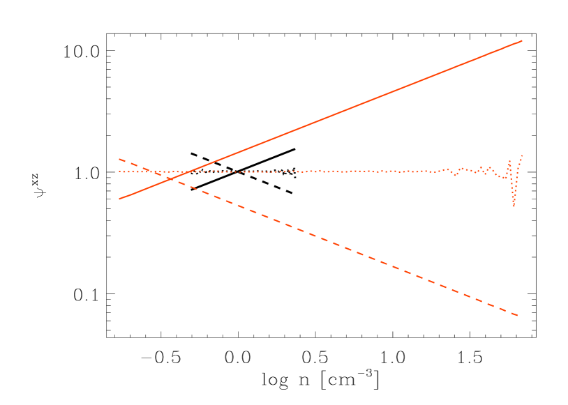
Figure 2.— Diagnostic Eq. (12) calculated by imposing an artificially generated magnetic field on top of the thermally stable hydrodynamic Run HDTSa (black lines) and thermally unstable Run HDSSa (orange/grey lines). Different types of magnetic field dependencies on density are plotted with different line styles: solid line, $|\bm{B}|=B_{0}\rho^{1/2}$, dashed line, $|\bm{B}|=B_{0}\rho^{-1/2}$, dotted line: random magnetic field.

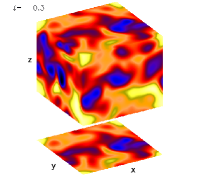
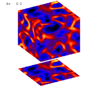
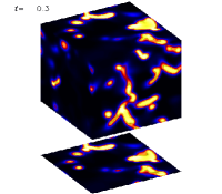
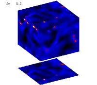
Figure 3.— Snapshots of the logarithmic density fields from different hydrodynamic runs at 250 Myrs. From left to right: HDTSa, HDTSc, HDSSa, HDSSc.

Figure 4.— Probability density functions for the thermally unstable hydrodynamic runs HDSSc (solid line) and HDSSa (dotted line), and the thermally stable hydrodynamic runs HDTSc (dashed line) and HDTSa (dashed-dotted line) at 250 Myrs of the simulation runs. On the left we show the PDF of logarithmic density, in the middle the PDF of logarithmic temperature, and on the right the PDF of logarithmic pressure.

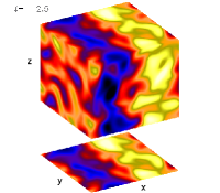
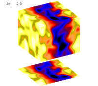
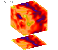
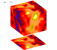
Figure 5.— Snapshots of the magnetic field strength from the thermally stable run TSa and thermally unstable run SSa at 2.5 Gyrs of evolution. From left to right: $B_{y}$ in TSa, $B_{z}$ in TSa, $B_{y}$ in SSa, and $B_{z}$ in SSa. The minimum value plotted with blue color corresponds to -1.2 $\mu$G and the maximum value to 1.2 $\mu$G, used in all plots.

3.1. Hydrodynamic state of the system

Let us first compare the purely hydrodynamic runs with different cooling functions and forcings. For the runs with thermally stable cooling functions (labeled with HDTS in Table 2), the formation of density structures occurs solely by the mixing and compression caused by the turbulent flow. For cases with the weakest forcing, Run HDTSa, rms-velocity of the order of 2 kms^-1, and density contrast of 3 is observed. The density field of this run at 250 Myrs is illustrated in Fig. 3 leftmost panel, from which it can easily be seen that the turbulence is so weak that the density structures generated by the flow do not show large contrasts and remain quite large in size. When the strength of the forcing is increased, the density contrast gets larger, as expected, so that in Run HDTSb, with 2.5 times stronger forcing, the contrast is roughly 20, and in Run HDTSc, with 3.5 times higher forcing, roughly 100, the respective rms-velocities being 6 and 8 kms^-1. The appearance of the flow field, illustrated in Fig. 3, the second panel from the left for Run HDTSc, has somewhat changed, the density structures generated now showing up as narrow filaments.

The effect of increasing forcing is also apparent in the probability distribution functions (hereafter PDFs) of the quantities, plotted in Fig. 4 for Run HDTSa (dashed-dotted lines) and Run HDTSc (dashed lines). Evidently, the distributions of all the quantities are all unimodal, with the width of them increasing as the forcing is increased. The density PDF is clearly reflecting the somewhat increased capability of the flow to generate denser structures with a smaller filling factor. The denser the structures the flow is capable of creating, the more will they cool, as the cooling term is of the form $\rho\Lambda$, modifying the rather symmetrical temperature PDF for Run HDTSa to exhibit an extended wing towards lower temperatures for Run HDTSc. This excess cooling will aid the dense regions in becoming denser, and a similar asymmetrical wing towards higher densities is seen in the density PDF for Run HDTSc. This is in agreement with the results of Passot & Vázquez-Semadeni (1998), who studied highly compressible polytropic flows with a varying Mach number. For polytropic indeces less than one, a very similar wing, approaching power-law behavior, was seen to develop towards higher densities. Similar, skewed density PDFs towards higher densities have also been reported from 3D-simulations of polytropic flows by Nordlund & Padoan (1999), interpreted to be caused by the effective $\gamma$ being reduced to below one in the regions of high compression.

For the runs with thermally unstable cooling functions (labeled with HDSS in Table 2), a major part of the formation of density structures is expected to occur due to the thermal instability, although the turbulence can also be expected to alter this picture considerably (see e.g. BKM07; Gazol et al., 2005). As can be seen from the two rightmost panels of Fig. 3, the appearance of the flow is very different from the thermally stable cases (the two leftmost panels in that figure). The action of the thermal instability leads to a very rapid (timescale of few tens of Megayears) segregation of the gas into cold cloudy and warm diffuse phases, the dense clouds clearly visible in the snapshots of the density field. Similarly to the thermally stable cases, the increasing vigor of turbulence can be seen to enhance the condensation process, so that excess cooling due to turbulent compression leads to an even larger density contrast and smaller structures.

We also plot the PDFs of the quantities for Run HDSSc (solid lines) and Run HDSSa (dotted lines) in Fig. 4. For the Run HDSSa with relatively weak forcing, the density and temperature distributions are still clearly bimodal, as has commonly been observed for thermally unstable flows, e.g. by BKM07, although large amounts of gas can be seen in the ’forbidden’ regime of thermally unstable temperatures with $\beta<1$. For the Run HDSSc, the bimodality of the density and temperature PDFs is much less pronounced; both distributions have become wider, and the peaks have been shifted towards higher densities and lower temperatures. This is reflected also in the peak of the pressure distribution. For the strongest forcing, the most probable pressure is somewhat higher than for the weaker forcing. A similar trend in the pressure distribution can also be seen in the thermally stable runs. The filling factor of the cold component gets considerably smaller as the forcing is increased, especially clearly seen when comparing the two leftmost panels of Fig. 3. This is also clearly manifested in the PDFs showing decreasing significance of the distribution of the cold phase. Due to the skewness of the density distribution towards higher densities, also the pressure distribution was asymmetric in the thermally stable case. In the thermally unstable cases, the pressure PDF is also clearly asymmetric, but in addition exhibits an extended wing towards the low pressures, and this wing gets more pronounced with increasing forcing amplitude, visible in the rightmost panel of Fig. 4. In our study, the vigor of forcing is still modest and the resulting Mach numbers are reasonably low in comparison to, e.g. Gazol et al. (2005), who studied a similar system in both the sub- and supersonic regimes. In their results, the signatures of TI in the PDFs are much less pronounced; on the other hand, the extended wing seen to develop in our pressure PDFs, is not reported in theirs.

As evident from Table 2, even though the cooling functions were scaled to produce the same integrated cooling over the whole temperature range for constant density, the thermal energy content in the thermally unstable runs is roughly half of that of the thermally stable counterparts. Obviously, this difference is due to the fact that the density is not constant, but actually very different in the thermally stable versus thermally unstable systems, as was discussed in length in this section, causing a nonlinear back-reaction to the cooling process, significantly enhancing its efficiency. For the thermally stable runs, however, the thermal energy is almost constant with any value of forcing investigated. For thermally unstable cases, the thermal energy is an increasing function of forcing.

3.2. Non-helical forcing

Using the same setup as for the hydrodynamic runs, we additionally include a very small random seed field of rms amplitude $B_{\rm init}=4\times 10^{-4}\mu$G and zero mean to the system, and follow the evolution of the system with the full set of MHD-equations with both cooling functions. In the following, we divide the magnetic field into its large-scale and fluctuating components, i.e. ${\bm{B}}^{\rm tot}={\bm{B}}+\bm{b}$, the condition $\left<\bm{b}\right>$=0 holding. In the runs TSanh-TScnh (thermally stable) and SSanh - SScnh (thermally unstable) the forcing function used has no relative helicity, i.e. $\sigma$=0. Large-scale dynamo action, i.e. the growth of the large-scale magnetic field $\bm{B}$ that has a non-zero mean, has been found in systems with non-helical forcing when large-scale shear has been included (Yousef et al., 2008). Systems such as the one studied here, however, can be expected to develop only small-scale dynamo action, i.e. the growth of the fluctuating component $\bm{b}$, when subjected to non-helical forcing. The results for the six non-helical runs produced are listed in Table 2. The forcing amplitude was increased as high as was permissible by the numerical scheme without invoking shock-capturing viscosities. No small-scale dynamo action was observed, i.e. the total magnetic field strength was exponentially decaying identically to the helical cases without large-scale dynamo action (see Fig. 7), in any of the runs, i.e. in the range of Reynolds numbers $31-97$. This indicates that in the system under investigation, the critical Reynolds number for small-scale dynamo action is larger than the ones reached in our runs, and that if magnetic fields are generated in the helical cases investigated, they arise solely due to the action of a large-scale dynamo.

Haugen et al. (2004) studied the onset of dynamo action in an isothermal system with non-helical forcing. As in this study, the vigor of forcing was increased, and it was observed that the critical Reynolds number for the onset of the small-scale dynamo was increasing with the Mach number. Shock-capturing viscosities were used to reach the trans- and supersonic regimes. For subsonic flows, the critical Reynolds number for small-scale dynamo action was of the order of 35, while for supersonic flows with Mach numbers exceeding unity, the critical Reynolds number was almost doubled up to 70. Our weakest forcing cases with modest Mach numbers have Reynolds numbers slightly below (TSanh, 31) or slightly exceeding the limit (SSanh, 39) found by Haugen et al. (2004), and in the light of their results, it is understandable that no small-scale dynamo action can be seen. The modest and high amplitude forcings used here do not yet produce Mach numbers even close to the supersonic limit, but their Reynolds numbers are clearly larger than the critical limits found by Haugen et al. (2004). Still, no small-scale dynamo action is seen, indicating that the inclusion of thermodynamics with the quite complex heating and cooling properties further alters the Mach-number dependence of the critical Reynolds number for small-scale dynamo action.

As can be seen from Table 2, the non-helical runs produce somewhat weaker turbulence than the runs with purely helical forcing $\sigma$=1. This is also reflected by the density distribution, so that the density contrast is reduced in the non-helical runs compared to the helical counterparts. This is manifested by smaller rms values for velocity, and thereby also smaller Reynolds numbers. The differences in the Reynolds numbers are not very large, so we believe that our conclusion about the absence of small-scale dynamo in the helical runs still holds.

Model	f	h	$\sqrt{\left<B_{x}^{2}\right>_{xz}}$	$\sqrt{\left<B_{x}^{2}\right>_{xy}}$	$\sqrt{\left<B_{y}^{2}\right>_{yz}}$	$\sqrt{\left<B^{2}_{y}\right>_{xy}}$	$\sqrt{\left<B^{2}_{z}\right>_{yz}}$	$\sqrt{\left<B^{2}_{z}\right>_{xz}}$
TSe	10	1	-	0.06	0.05	0.07	0.05	-
TSa	20	1	-	-	0.49	-	0.43	-
TSd	35	1	0.70	-	-	-	-	0.79
TSb	50	1	0.98	-	-	-	-	1.01
TSc	70	1	-	1.18	-	1.23	-	-
SSf	15	1	-	0.09	-	0.09	-	-
SSa	20	1	-	-	0.21	-	0.23	-
SSb	50	1	0.58	-	-	-	-	0.60
SSc	70	1	-	0.80	-	0.81	-	-

Table 3The rms-stregth of the $k=1$-mode, measured in $\mu$G, generated in the runs.

3.3. Thermally stable magnetohydrodynamic runs

Next we repeat the magnetohydrodynamic runs with helical forcing, starting with the thermally stable cooling function, which is expected to produce large-scale dynamo action (e.g. Brandenburg, 2001). The Run TSf with the forcing amplitude $f=7$ is sub-critical to dynamo action, i.e. the small seed field exponentially decays. The Run TSe with $f=10$, however, produces a very slowly growing magnetic field, with the time scale of growth of roughly $500$ Myrs. The growth of the field saturates only after 4 Gyrs, the saturation energy being less than half of the kinetic energy of turbulence. Inspecting the Reynolds numbers realized in Runs TSe and TSf from Table 2, the critical Reynolds number for the large-scale dynamo in this system, therefore, is roughly between 12-16.

Runs with higher forcing (Runs TSa, TSd, TSb and TSc), with a forcing ranging between 20-70, all produce dynamo action that leads to the generation of magnetic fields, the energy of which is in rough equipartition with the kinetic energy of turbulence for intermediate forcings (TSa and TSd), but slightly lower than the equipartition value for the highest forcings investigated (TSb and TSc). The growth rate and saturation strength of the field are increasing as function of increasing forcing, and thereby also as functions of the Reynolds number Rm, so that for the highest forcing investigated, the time scale of growth is roughly 27 Myrs, building up the magnetic field in a few hundreds of Myrs. A similar, but isothermal, system has been investigated earlier by Brandenburg (2001), who found otherwise similar behavior, but the energy of the magnetic fields generated in the system exceeded the kinetic energy of turbulence. The build-up of the large-scale field from the equipartition to the super-equipartition values was observed to occur on the diffusive timescale, and therefore be dependent on Rm. Such behavior is not seen in the system of this study.

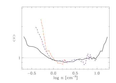
Figure 6.— The calculated flux diagnostic $\left<\Psi\right>$ from Eq.(12) for the thermally stable run TSa (dashed-dotted), TSd (dashed) and TSc (solid line).

Next, we study the spatial distribution of the magnetic fields, and convince ourselves that the dynamo seen in the helical forcing case is indeed of the large-scale type, being capable of generating magnetic fields on spatial scales larger than the forcing scale of the turbulence, $k_{f}/k_{1}=3$. In the two leftmost panels of Fig. 5, we plot two components of the magnetic field for Run TSa after the growth of the magnetic field has saturated. For the $B_{y}$ component, a clear sinusoidal wave of the Fourier mode $k=1$ over the $x$-coordinate is seen, while $B_{z}$ shows the same mode with a cosinus dependence of the spatial coordinate. The patterns seen are very similar to the study of Brandenburg (2001), and the field is clearly coherent over larger scales as the forcing scale. Such a mean field vanishes when averaging over the whole volume, but the rms-strength of the large-scale component $\sqrt{\left<B_{y}^{2}\right>_{yz}}$ can be recovered if averaging over $y$- and $z$-directions, denoted with $\left<\right>_{yz}$, is used; we use averaging of this type in Table 3 to estimate the generated large-scale field strengths.

The scales of the large-scale fields are the same for all the runs independent of forcing, but the direction of the generated mean field varies almost from one run to another. As can been seen from Table 3, the weakest forcing case, Run TSf, the Reynolds number being very close to the marginal one and the time scale of growth very long, exhibits mean fields in every direction. Run TSa, the magnetic field shown in Fig. 5, develops strong mean components of $B_{y}$ and $B_{z}$ in the $x$-direction. The intermediate forcing cases, Runs TSd and TSb, on the other hand, show mean components of $B_{x}$ and $B_{z}$ over the $y$-direction. Finally, the strongest forcing case, Run TSc, develops the strongest mean fields in $B_{x}$ and $B_{y}$ over the $z$-direction. Also in the isothermal study of Brandenburg (2001), any direction of the mean field could be preferred, only depending on the fine details of the initial random distribution. As is evident when comparing the rms values of the total magnetic field, presented in Table 2, to the strength of the mean component in Table 3, almost all magnetic energy is contained in the $k=1$ mode. As the forcing is increased, small contribution of the small-scale field is generated, but in all cases investigated this contribution is negligible, verifying the assumption that no small-scale dynamo is present in the models.

When calculating the flux diagnostic, defined by Eq. (12), for a magnetic field with a mean component at the wavenumber $k=1$ over a certain direction, having different signs and roughly equal magnitudes in the different halves of the box, the total magnetic flux would evidently be close to zero. Therefore, we need to use absolute values of the field strength, $\left|\bm{B}\right|$, in Eq. 12. Furthermore, as the distribution of the mean fields can be quite complex, we calculate an average value $\left<\Psi\right>$ of $\Psi^{xy}$, $\Psi^{yz}$, and $\Psi^{xz}$. In Fig. 6 we show plots of the magnetic flux diagnostic for the thermally stable runs developing dynamo action. For the weakest forcing case, Run TSa, the magnetic and density fields show signs of anti-correlation for low densities, $n<1$cm^-3, and no clear correlation for densities above that limit. The anti-correlation at lower densities is observed to decrease with increasing forcing and dynamo efficiency, but only for the highest forcing and most efficient dynamo, Run TSc, are signs of positive correlation at higher densities, 10-35 cm^-3, established. This clearly shows that the compression due to the forcing alone is very inefficient in producing any significant positive correlation between the density and magnetic field.

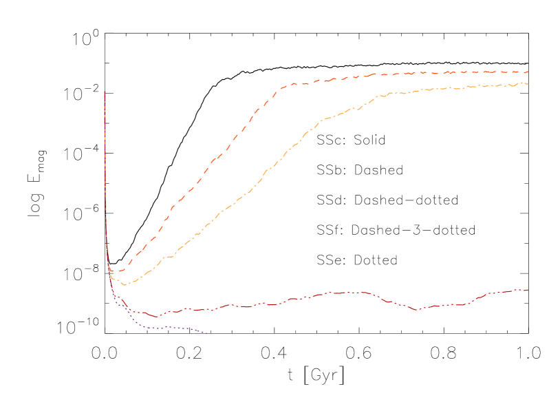
Figure 7.— Time evolution of the magnetic fields in some of the thermally unstable runs.

Figure 8.— Left panel: Thermal energies and the ratio of magnetic to kinetic energy as function of magnetic Reynolds number for runs with different cooling functions. Stars: thermal energy in the thermally stable MHD Runs TSf – TSc. Crosses: thermal energy in the thermally unstable MHD Runs SSf – SSc. Diamonds: magnetic to kinetic energy ratio in Runs TSf–TSc. Triangles: magnetic to kinetic energy ratio in Runs SSf–SSc. Right panel: Density contrast $\Delta\rho$ from MHD runs (stable with stars, unstable with diamonds) compared with their hydrodynamic counterparts (stable with crosses, unstable with traingles) as function of the forcing amplitude, $f$.

Figure 9.— Probability density functions for the thermally unstable hydrodynamic runs HDSSc (solid line) compared with the magnetohydrodynamic counterpart SSc (dashed line), and HDSSb (dotted line) with SSb (dashed-dotted line). On the left we show the PDF of logarithmic density, in the middle the PDF of logarithmic temperature, and on the right the PDF of logarithmic pressure.

3.4. Thermally unstable magnetohydrodynamic runs

Finally, we produce magnetohydrodynamic runs with helical forcing using the thermally unstable cooling function, the results being listed in the lower part of Tables 2 and 3 and the time evolution of the magnetic energy for some runs shown in Fig. 7. As is evident from this table, when comparing these runs with their thermally stable counterparts with the same magnitude of forcing, it can be noted that the turbulence is more vigorous with the thermally unstable cooling function in the sense that rms values of velocity and Reynolds numbers are larger for any fixed forcing amplitude. The kinetic energy, however, is smaller for the thermally unstable runs than for the thermally stable ones, explained by the density distribution being dominated by the warm diffuse gas with low density for the thermally unstable setup.

For the Run SSf with the forcing amplitude $f$=15 producing turbulence with $\mbox{Rm}\approx 45$, a very slowly growing dynamo is found, as seen from Fig. 7, whereas the magnetic field of the Run SSe with $\mbox{Rm}\approx 28$ is seen to decay exponentially. The critical Reynolds number, therefore, lies somewhere in between 28–45, roughly twice the value found for the thermally stable runs. In other words, the large-scale dynamo is harder to excite in the thermally unstable system. As is evident from the left panel of Fig. 8, where we plot the dependence of thermal energy and the ratio of magnetic to kinetic energy ratio on the magnetic Reynolds number Rm, the magnetic energy in the saturated state remains below the kinetic energy of turbulence up to the forcing amplitude $f$=35 in Run SSd, for which the Reynolds number is 58. For the thermally stable runs the dynamo efficiency of this level was reached with $f$=20 with Rm=27, the difference being again by a factor of two. For the strongest forcings investigated (Runs SSb and SSc), the magnetic energy exceeds the kinetic energy of turbulence. Such behavior was not seen in the thermally stable runs.

The density contrast can be seen to become affected by the presence of the magnetic field; this effect is visible in Fig. 8 right panel, where we plot $\Delta\rho$ both for the MHD runs and their hydrodynamic counterparts. For both the stable and unstable runs the trend appears very similar: as long as the magnetic field energy remains clearly below the kinetic energy of turbulence, i.e. the dynamo efficiency is still low, the density contrast becomes enhanced. For forcings capable of generating a magnetic field close to or exceeding the kinetic energy of turbulence (Runs TSc, SSb, and SSc) the density contrast becomes reduced. This can be interpreted as the lowered capability of either the turbulence or the condensation mode of the thermal instability to create density structures in the presence of a strong dynamo-generated magnetic field, in agreement with the results from earlier magnetohydrodynamic studies without self-consistent dynamo action, e.g. by Ostriker et al. (1999) and Padoan & Nordlund (1999).

In Fig. 9 we show PDFs of the magnetohydrodynamic runs with the strongest forcings (Runs SSb and SSc) compared to the hydrodynamic counterparts (Runs HDSSb and HDSSC). The main effect due to the presence of the magnetic field seen in them is the decreased amount of dense gas at the very high end of the density distribution, and a slight increase of very low density gas for Run SSc, while hardly any difference can be seen in the temperature distributions. The pressure PDF, therefore, reflects the decreased densities, the higher pressure wing being reduced for both Runs SSb and SSc. This implies that the stronger the magnetic field grows, the more it resists the cloud compression due to thermal instability. In a similar study, Gazol et al. (2009) reported that an initially uniform magnetic field of varying strengths caused an extended low-pressure wing to their pressure distribution; in our case, the wing was seen already in the hydrodynamic regime, and the effect of the magnetic field on it is barely visible. In a related, but not completely comparable, study by de Avillez & Breitschwerdt (2005), the effect of the presence of a magnetic field on a supernova-regulated flow was studied. In contrast to our results, the amount of cold and dense gas was observed to increase in the magnetohydrodynamic versus the hydrodynamic setup. The differences seen between our model to the other two might be connected to the fact that in our case self-consistently dynamo-active flows were studied in contrast to imposed ones passively advected by the flow.

Finally, we plot the flux diagnostic $\left<\Psi\right>$ for the dynamo-active thermally unstable runs in Fig. 10. If compared to the corresponding plot for thermally stable runs, Fig. 6 showing uncorrelated density and magnetic fields except for the high-density end of the run with the highest forcing, the action of thermal instability on the system produces clear positive correlation between the two quantities. The correlation for all the cases investigated is considerably weaker, of the form $B\propto\rho^{0.2}$ (thick line plotted in the figure), compared to the one observed in the interstellar matter. The strongest correlation is seen for the Run SSd, the trend declining somewhat for higher forcings. For all the runs, there seems to be a tendency for the correlation to break down at the highest densities.

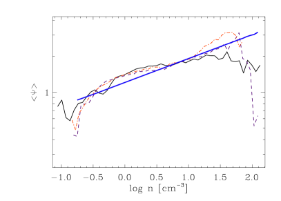
Figure 10.— The calculated flux diagnostic $\left<\Psi\right>$ from Eq.(12) for the thermally unstable runs SSd (dashed-dotted), SSb (dashed) and SSc (solid line). The thickest line shows a fit of the type $B\propto\rho^{0.2}$.

4. Conclusions

In this paper we have investigated the role of thermal instability for large-scale dynamo action in galaxies and in producing the density-magnetic field correlation in the interstellar matter. A periodic cubic magnetohydrodynamic setup with external helical forcing was used to establish large-scale dynamo action in the system, which was subject either to thermally stable or unstable cooling functions having the same integrated net cooling for constant density. Reference runs without magnetic fields and with non-helical forcing were made, the former to isolate the effect of the magnetic fields on the system, and the latter for detecting if small-scale dynamo action was produced in the Reynolds number regime investigated. The latter set of runs showed that no small-scale dynamo action was to be expected in the helical runs, the critical Reynolds number for small-scale dynamo action in this particular system being larger than 97. This number is larger than obtained in similar, but isothermal, setups investigated.

In the thermally stable runs, the critical Reynolds number of large-scale dynamo action was calculated to be in between 12-16, whereas for the thermally unstable setup the corresponding range was found to be roughly twice that, 28-45; the thermal instability, therefore, makes the onset of the large-scale dynamo harder. In contrast to the thermally stable cases investigated, that were observed to produce magnetic fields in equipartition with the kinetic energy of turbulence, the thermally unstable ones were capable of producing magnetic fields with somewhat larger energy than contained in the turbulent velocity field. In terms of the rms-magnetic field strength, the thermally stable runs produced roughly 1.5 times larger magnetic fields than the thermally unstable counterparts per fixed forcing, the maximal values being of the order of 1.5$\mu$G for the strongest forcing. The dynamos, no matter which cooling function was used, always produced magnetic fields with a mean component at the wavenumber $k$=1. The large-scale field could be generated in any direction, and show systematic variation over any spatial coordinate, depending on the strength of the forcing.

In the thermally stable runs the denser structures were formed due to the action of the turbulent velocity field itself. The enhanced density contrast produced by increasing forcing, however, was found to be very inefficient in producing a density-magnetic field correlation in the system. In fact, a positive correlation was found only for the highest forcing case investigated, and even then only at the limit of the highest densities. For all the other cases, our flux diagnostic indicated a tendency for uncorrelation between the quantities. For the thermally unstable dynamo-active cases investigated, a positive correlation of the form $B\propto\rho^{0.2}$ was observed to be established, but a tendency of this rather weak correlation to break down at the high density limit was seen. It can be concluded that an instability of any ’condensation’ type, i.e. the gravitational or condensation mode of thermal instability, is instrumental in establishing density-magnetic field correlation in the ISM, but based on this study, the correlation predicted due to thermal instability is weak, and especially so for high densities.

References

- Audit & Hennebelle (2005) Audit, E., & Hennebelle, P. 2005, A&A, 433, 1
- Balsara et al. (2004) Balsara, D. S., Kim, J., Low, M.-M. M., & Matthews, G. J. 2004, ApJ, 617, 339
- Banerjee et al. (2009) Banerjee, R., Vázquez-Semadeni, E., Hennebelle, P., & Klessen, R. S. 2009, MNRAS, 398, 1082
- Beck et al. (2005) Beck, R., Fletcher, A., Shukurov, A., Snodin, A., Sokoloff, D. D., Ehle, M., Moss, D., & Shoutenkov, V. 2005, A&A, 444, 739
- Brandenburg (2001) Brandenburg, A. 2001, ApJ, 550, 824
- Brandenburg & Dobler (2002) Brandenburg, A., & Dobler, W. 2002, Computer Physics Communications, 147, 471
- Brandenburg et al. (2007) Brandenburg, A., Korpi, M. J., & Mee, A. J. 2007, ApJ, 654, 945
- Brandenburg et al. (1995) Brandenburg, A., Nordlund, A., Stein, R. F., & Torkelsson, U. 1995, ApJ, 446, 741
- Chiang & Prendergast (1985) Chiang, W.-H., & Prendergast, K. H. 1985, ApJ, 297, 507
- Cox (2005) Cox, D. P. 2005, ARA&A, 43, 337
- Crutcher (1999) Crutcher, R. M. 1999, ApJ, 520, 706
- de Avillez (2000) de Avillez, M. A. 2000, MNRAS, 315, 479
- de Avillez & Breitschwerdt (2005) de Avillez, M. A., & Breitschwerdt, D. 2005, A&A, 436, 585
- Ferrière (2001) Ferrière, K. M. 2001, ApJ, 73, 1031
- Field (1965) Field, G. B. 1965, ApJ, 142, 531
- Field et al. (1969) Field, G. B., Goldsmith, D. W., & Habing, H. J. 1969, ApJ, 155, L149
- Fletcher et al. (2010) Fletcher, A., Beck, R., Shukurov, A., Berkhuijsen, E. M., & Horellou, C. 2010, ArXiv e-prints
- Gammie (2001) Gammie, C. F. 2001, ApJ, 553, 174
- Gazol et al. (2009) Gazol, A., Luis, L., & Kim, J. 2009, ApJ, 693, 656
- Gazol et al. (2005) Gazol, A., Vázquez-Semadeni, E., & Kim, J. 2005, ApJ, 630, 911
- Gazol-Patiño & Passot (1999) Gazol-Patiño, A., & Passot, T. 1999, ApJ, 518, 748
- Gressel et al. (2008) Gressel, O., Elstner, D., Ziegler, U., & Rüdiger, G. 2008, A&A, 486, L35
- Haugen et al. (2004) Haugen, N. E. L., Brandenburg, A., & Mee, A. J. 2004, MNRAS, 353, 947
- Hawley et al. (1995) Hawley, J. F., Gammie, C. F., & Balbus, S. A. 1995, ApJ, 440, 742
- Heiles & Crutcher (2005) Heiles, C., & Crutcher, R. 2005, in Lecture Notes in Physics, Berlin Springer Verlag, Vol. 664, Cosmic Magnetic Fields, ed. R. Wielebinski & R. Beck, 137
- Heitsch et al. (2005) Heitsch, F., Burkert, A., Hartmann, L. W., Slyz, A. D., & Devriendt, J. E. G. 2005, ApJ, 633, L113
- Heitsch & Hartmann (2008) Heitsch, F., & Hartmann, L. 2008, ApJ, 689, 290
- Heitsch et al. (2004) Heitsch, F., Zweibel, E. G., Slyz, A. D., & Devriendt, J. E. G. 2004, ApJ, 603, 165
- Hennebelle et al. (2008) Hennebelle, P., Banerjee, R., Vázquez-Semadeni, E., Klessen, R. S., & Audit, E. 2008, A&A, 486, L43
- Inutsuka & Koyama (2007) Inutsuka, S., & Koyama, H. 2007, in Astronomical Society of the Pacific Conference Series, Vol. 365, SINS - Small Ionized and Neutral Structures in the Diffuse Interstellar Medium, ed. M. Haverkorn & W. M. Goss, 162
- Käpylä & Brandenburg (2009) Käpylä, P. J., & Brandenburg, A. 2009, ApJ, 699, 1059
- Korpi et al. (1999) Korpi, M. J., Brandenburg, A., Shukurov, A., Tuominen, I., & Nordlund, Å. 1999, ApJ, 514, L99
- Koyama & Initsuka (2004) Koyama, H., & Initsuka, S. 2004, ApJ, 602, L25–L28
- Koyama & Inutsuka (2002) Koyama, H., & Inutsuka, S. 2002, ApJ, 564, L97
- Kritsuk & Norman (2002) Kritsuk, A. G., & Norman, M. L. 2002, ApJ, 569, L127
- McKee & Ostriker (1977) McKee, C. F., & Ostriker, J. P. 1977, ApJ, 218, 148
- Myers et al. (1995) Myers, P. C., Goodman, A. A., Gusten, R., & Heiles, C. 1995, ApJ, 442, 177
- Nordlund & Padoan (1999) Nordlund, Å. K., & Padoan, P. 1999, in Interstellar Turbulence, ed. J. Franco & A. Carraminana, 218–+
- Norman & Ferrara (1996) Norman, C. A., & Ferrara, A. 1996, ApJ, 467, 280
- Ostriker et al. (1999) Ostriker, E. C., Gammie, C. F., & Stone, J. M. 1999, ApJ, 513, 259
- Padoan & Nordlund (1999) Padoan, P., & Nordlund, Å. 1999, ApJ, 526, 279
- Passot & Vázquez-Semadeni (1998) Passot, T., & Vázquez-Semadeni, E. 1998, Phys. Rev. E, 58, 4501
- Passot & Vázquez-Semadeni (2003) —. 2003, A&A, 398, 845
- Piontek & Ostriker (2005) Piontek, R. A., & Ostriker, E. 2005, ApJ, 629, 849
- Piontek & Ostriker (2007) —. 2007, ApJ, 663, 183
- Rosen et al. (1993) Rosen, A., Bregman, J. N., & Norman, M. L. 1993, ApJ, 413, 137
- Santos-Lima et al. (2010) Santos-Lima, R., Lazarian, A., de Gouveia Dal Pino, E. M., & Cho, J. 2010, ApJ, 714, 442
- Troland & Heiles (1986) Troland, T. H., & Heiles, C. 1986, ApJ, 301, 339
- Vázquez-Semadeni et al. (2000) Vázquez-Semadeni, E., Gazol, A., & Scalo, J. 2000, ApJ, 540, 271
- Vázquez-Semadeni et al. (2006) Vázquez-Semadeni, E., Ryu, D., Passot, T., González, R. F., & Gazol, A. 2006, ApJ, 643, 245
- Yousef et al. (2008) Yousef, T. A., Heinemann, T., Schekochihin, A. A., Kleeorin, N., Rogachevskii, I., Iskakov, A. B., Cowley, S. C., & McWilliams, J. C. 2008, Physical Review Letters, 100, 184501