First evidence for a gravitational lensing-induced echo in gamma rays with Fermi LAT

Abstract

Aims. This article shows the first evidence for gravitational lensing phenomena in high energy gamma-rays. This evidence comes from the observation of a gravitational lens induced echo in the light curve of the distant blazar PKS 1830-211.

Methods. Traditional methods for the estimation of time delays in gravitational lensing systems rely on the cross-correlation of the light curves of the individual images. In this paper, we use 300 MeV-30 GeV photons detected by the Fermi-LAT instrument. The Fermi-LAT instrument cannot separate the images of known lenses. The observed light curve is thus the superposition of individual image light curves. The Fermi-LAT instrument has the advantage of providing long, evenly spaced, time series. In addition, the photon noise level is very low. This allows to use directly Fourier transform methods.

Results. A time delay between the two compact images of PKS 1830-211 has been searched for both by the autocorrelation method and the “double power spectrum” method. The double power spectrum shows a 3 $\sigma$ evidence for a time delay of 27.5$\pm$1.3 days, consistent with the result from Lovell et al. (1998). The relative uncertainty on the time delay estimation is reduced from 20% to 5%.

1 Introduction

The precise estimation of the time delay between components of lensed Active Galactic Nuclei (AGN) is crucial for modeling the lensing objects. In turn, more accurate lens models give better constraints on the Hubble constant. More than 200 strong lens systems have been found. Most of them were discovered in recent years by dedicated surveys such as the Cosmic Lens All-Sky Survey (Myers et al. 2003; Browne et al. 2003) and the Sloan Lens ACS Survey (Bolton et al. 2004). The launch of the Fermi sattelite (Atwood et al. 2009) in 2008 gives the opportunity to observe gravitational lensing phenomena with high energy gamma rays. The observation strategy of Fermi-LAT, which surveys the whole sky in 190 minutes, allows a regular sampling of quasar light curves with a period of a few hours. Since the launch of the Fermi satellite, the LAT instrument has been collecting high energy photons for more than 800 days. This paper deals with the observation and estimation of time delays of strong lensing systems and not with the detection and use of microlensing phenomena as in Torres et al. (2003).

The multiple images of a gravitational lensed AGN cannot be directly observed with the high energy gamma-ray instruments such as the Fermi-LAT, Swift or ground based Cerenkov telescopes, due to their limited angular resolutions. The angular resolution of these instruments is at best of a few arcminutes (in the case of HESS), when the typical separation of the images for quasar lensed by galaxies is a few arcseconds. Since the multiple images cannot be observed, methods based on the detection of an echo in the light curve are studied in this paper. The observed signal is the superposition of the intrinsic light curve of the AGN and at least one delayed copy of this light curve, with a different amplitude.

The method has been tested on simulated light curves and on Fermi observations of the very bright radio quasar PKS 1830-211, for which the time delay has been accurately measured by Lovell et al. (1998) using radio observations. The paper is organized as follows: we first give a very brief summary of properties of PKS 1830-211 and of Fermi LAT data towards this AGN. Then we introduce the methods for time delay estimation. The last section is devoted to the measurement of the time delay between the two compact components of PKS 1830-211.

2 The PKS 1830-211 gravitational lens

The AGN PKS 1830-211 is a variable, bright radio source and an X-ray blazar. Its redshift was measured to be z=2.507 (Lidman et al. 1999). The blazar was detected in the $\gamma$-ray wavelengths with EGRET. The association of the EGRET source with the radio source was done by Mattox et al. (1997). The classification of PKS 1830-211 as a gravitational lensed quasi-stellar object was first proposed by Pramesh Rao & Subrahmanyan (1988).

Two potential lenses have been identified along the line of sight to PKS 1830-211 by the observation of molecular absorption at centimeter and millimeter wavelengths. One possible lensing object is a galaxy at redshift z=0.19 (Lovell et al. 1996), and the other a galaxy at redshift z=0.89 (Wiklind & Combes 1996). According to Winn et al. (2002), the actual lens is the galaxy at redshift z=0.89.

PKS 1830-211 is observed in radio as an elliptical ring-like structure connecting 2 bright sources distant of roughly one arcsecond (Jauncey et al. 1991). The compact components were separately observed by the Australia Telescope Compact Array at 8.6 GHz for 18 months. These observations and the subsequent analysis made by Lovell et al. (1998) gave a magnification ratio between the 2 images equal to $1.52\pm 0.05$ and a time delay of $26^{+4}_{-5}$ days.

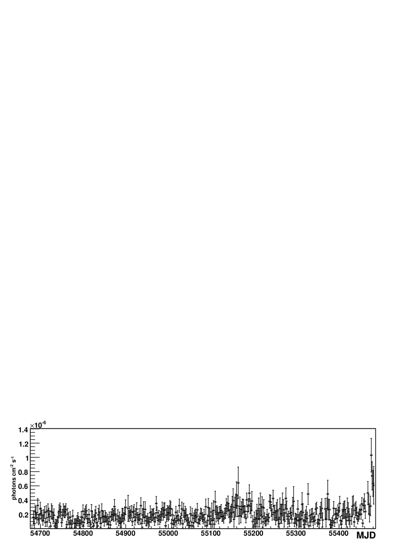
Figure 1: Fermi LAT light curve of PKS 1830-211, with a 2 days binning. The energy range is 300 MeV to 300 GeV.

2.1 Fermi LAT data on PKS 1830-211

PKS 1830-211 has been detected by the Fermi-LAT instrument with a detection significance above 41 Fermi Test Statistic (TS), equivalent to a 6 $\sigma$ effect (Abdo et al. 2010). The long-term light curve is presented on figure 1 with a 2 days binning. The data analysis from this paper uses a 2 days binning, which provides a sufficient photon statistic per bin with a time span per bin much shorter than 28 days. The data analysis was cross-checked by binning the light-curve into 1 day and 23 hours bins, with similar results. The data were taken between August 4 2008 and October 13 2010, and processed by the publicly available Fermi Science Tools version 9. The v9r15p2 software version and the P6_V3_DIFFUSE instrument response functions have been used. The light curve has been produced by an aperture photometry selecting photons from a region with radius 0.5 deg around the nominal position of PKS 1830-211 and energies between 300 MeV and 300 GeV.

3 Data processing and method

3.1 Idea

If a distant source (in our case an AGN) is gravitationally lensed, the light reaches the observer through at least 2 different paths. We assume here that there are only 2 light paths. In reality, the light curves of the 2 images are not totally identical since (in addition to differences due to photon noise) the source can be microlensed in one of the two paths. In this paper, we neglect this effect. Neglecting for the moment the background light, the observed flux can be decomposed into 2 components. The first component is the intrinsic AGN light curve, given by $f(t),$ with Fourier transform $\tilde{f}(\nu).$ The second component has a similar time evolution than the first one, but is shifted in time with a delay $a.$ In addition, the brightness of the second component differs by a factor of $b$ from that of the first component, so that it can be written as $bf(t+a)$ and its transform to the Fourier space gives $b\tilde{f}(\nu)e^{-2\pi i\nu a}$.

The sum of two component gives $g(t)=f(t)+bf(t+a)$ which transforms into $\tilde{g}(\nu)=\tilde{f}(\nu)(1+be^{-2\pi i\nu a})$ in Fourier space.

The power spectrum $P_{\nu}$ of the source is obtained by computing the square modulus of $\tilde{g}(\nu).$

$$P_{\nu}=|\tilde{g}(\nu)|^{2}=|\tilde{f}(\nu)|^{2}(1+b^{2}+2bcos(2\pi\nu a))$$ (1)

The measurable $P_{\nu}$ is the product of the “true” power spectrum of the source times a periodic component with a period (in the frequency domain) equal to the inverse of the relative time delay $a$.

The usual way of measuring the time delay $a$ is to calculate the autocorrelation function of f(t). This method was investigated by Geiger & Schneider (1996). The autocorrelation function can be written as the sum of three terms. One of this term describes the intrinsic autocorrelation of the AGN, decreasing with a time constant $\lambda$. If $\lambda$ is larger than $a$, the autocorrelation method fails, because the time delay peak merges with the intrinsic component of the AGN. Another potential problem with the autocorrelation method is the sensitivity to spurious periodicities such as the one coming from the motion and rotation of the Fermi satellite.

The periodic modulation of $P_{\nu}$ suggests the use of another method, based on the computation of the power spectrum of $P_{\nu}$, noted $D_{a}$. This method is similar in spirit to the cepstrum analysis (Bogert et al. 1963) used in seismology and speech processing. If $|\tilde{f}(\nu)|^{2}$ was a constant function of $\nu$, $D_{a}$ would have a peak at the time delay $a$. In the general case, $D_{a}$ is obtained by the convolution of a Dirac function, coming from the cosinus modulation, by the Fourier transform of the function:

$$\tilde{h}(\nu)=\tilde{f}(\nu)Window(0,W)$$ (2)

where Window(0,W) is the window in frequency of $P_{\nu}$ and W is maximum available frequency. The Fourier transform h(a) of $\tilde{h}(\nu)$ defines the width of the time delay peak in the double power spectrum $D_{a}$.

For instance if $\tilde{f}(\nu)=e^{-\lambda\nu}$ and $\lambda W>>1,$ then the time delay peak in $D_{a}$ has a Lorentzian shape with a FWHM of ${\lambda}/{\pi}.$ For a typical value of $\lambda=10$ days, one has a FWHM of 3 days.

In next section we describe the calculation of $P_{\nu}$ and $D_{a}$ and illustrate the procedure with Monte Carlo simulations.

3.2 Power Spectrum

The Fourier transform is a powerful technique to analyze astronomical data, but it requires a proper preparation of the observations. To avoid problems arising from the finite length of measurements, sampling and aliasing, we use the procedure for data reduction described by Brault & White (1971).

We start with dividing the whole light curve into several segments of equal length. The data have to be evenly spaced and the number of points per segment needs to be equal to a power of 2. The choice of the segment length is compromise between the spectral resolution and the size of error bars on points in the spectrum. The resolution of lines increases with the number of points in the segment, but the error on each point in the spectrum decreases as the number of segments.

As suggested by Brault & White (1971), the segments are overlapped to obtain a larger number of segments with a sufficient number of points. Then the data in each segment are transformed with the following procedure:

1. Data gaps are removed by linear interpolation

2. The mean is subtracted from the series to avoid having a large value in the first bin of the transform

3. The data are oversampled to remove aliasing.

4. Zeros are added to the end of the series to reduce power at high frequencies

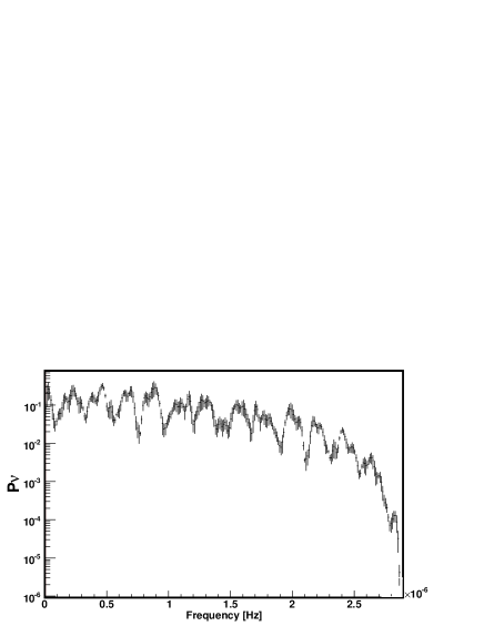
Figure 2: Simulated power spectrum of a lensed AGN with a time delay between images of 28 days. The power $P_{\nu}$ is in arbitrary units.

Finally, the power spectrum is averaged over all segments. The power spectrum obtained with an artificial light curve is shown on figure 2.

The artificial light curve was produced by summing three simulated components. The light curve of PKS 1830-211 shown on figure 1 does not exhibit any easily recognizable features, but has a rather random-like aspect. The first component was thus simulated as a white noise, with a Poisson distribution. It would be more realistic to use red noise instead of white noise but the latter is sufficient for most of our purposes, such as computing $D_{a}.$ The second component is obtained from the first by shifting the light curve with a 28 days time lag. The effect of differential magnification of the images has also been included. The background photon noise was taken into account by adding a third component with a Poisson distribution.

The mean number of counts per 2 day bin for PKS 1830-211 is 5.42 counts. This value was used for the simulation of the artificial light curve. The first and second component contribute 80% of the simulated count rate and the rest is contributed by the noise component.

To get a simulated flux similar to the observed flux, the simulated count rate is divided by the average exposure from observations ( $2.8557\ 10^{7}\ s\ cm^{2}$).

3.3 Time Delay Determination

The methods of time delay determination use the power spectrum $P_{\nu}$ obtained as described in the previous section. The simulated $P_{\nu}$ presented on figure 2 shows a very clear periodic pattern. From equation 1 we know that the period of the observed wobbles corresponds to inverse of the time delay between the images.

Our preferred approach was to calculate the double power spectrum $D_{a}$. As in section 3.2, the power spectrum $P_{\nu}$ has to be prepared before undergoing a Fourier transform to the “time delay” domain.

The low frequency part ($\nu<1/55\mbox{day}^{-1}$) of $P_{\nu}$ is cut off. This cut arises because of the large power observed low frequencies in the power spectrum of PKS 1830-211. The high frequency part of the spectrum $P_{\nu}$ is also removed because the power at high frequency is small (it goes to 0 at the Nyquist frequency). The calculation of $D_{a}$ proceeds like in section 3.2, except that the $P_{\nu}$ data are bend to zero by multiplication with a cosine bell. This eliminates spurious high frequencies, when zeros are added to the $P_{\nu}$ series. The $D_{a}$ distribution is estimated from 5 segments of the light curve. In every bin of the $D_{a}$ distribution, the estimated double power spectrum is given by the average over the 5 segments. The errors bars on $D_{a}$ are estimated from the dispersion of bin values divided by 2 (since there are 5 segments). Due to the random nature of the sampling process, some of the error bars obtained are much smaller than the typical dispersion in the $D_{a}$ points. To take this into account, a small systematic error bar was added quadratically to all points. The result (with statistical error bars only) is presented on figure 3.

As described in section 3.2, we simulated light curves with a time delay of 28 days. A peak is apparent near a time delay of 28 days on the $D_{a}$ distribution shown on figure 3. The points just outside the peak are compatible with a flat distribution. Including also the points in the peak gives a distribution which is incompatible with a flat distribution at the 10 sigma level.

The parameters of the peak were determined by fitting the sum of a linear function for the background plus a Gaussian function for the signal. In the case shown on figure 3, the time delay estimated from $D_{a}$ is $27.94\pm 0.61$ days.

As mentioned in section 3.1, the usual approach for the time delay estimation is to compute the autocorrelation of the light curve. The auto-covariance is obtained by taking the real part of the inverse Fourier transform of $P_{\nu}$. The auto-covariance is normalized (divided by the value at zero time lag) to get the autocorrelation. The autocorrelation function of an artificial light curve simulated as in section 3.2 is presented on figure 4.

A peak with a significance of roughly 16 $\sigma$ is present at $27.85\pm 0.14$ days. However the significance of this peak is overestimated since light curves are simulated with white noise instead of red noise. The autocorrelation function of a light curve driven by red noise is given by $e^{-a/\lambda}.$ In the case of our simulated light curves, $\lambda=0$, so that the peak is a little affected by the background of the AGN.

For the simulated light curves, both approaches of time delay determination give reasonable and compatible results.

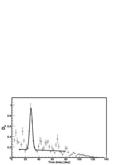
Figure 3: Double power spectrum $D_{a}$ for the simulated lensed AGN of figure 2. $D_{a}$ is plotted in arbitrary units. The solid line is a fit to a linear plus Gaussian profile.

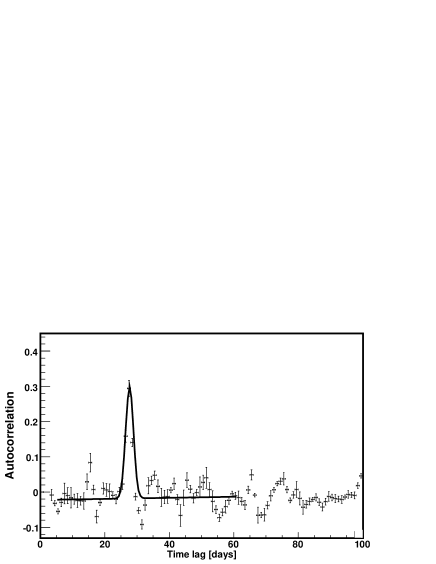
Figure 4: Autocorrelation function of the simulated lensed AGN of figure 2. The solid line is a fit to a linear plus Gaussian profile.

4 Results and Discussion

The results for real data were obtained with the same procedure as was presented for the simulated light curves. Figure 5 shows the power spectrum $P_{\nu}$ calculated from the light curve of PKS 1830-211. A periodic pattern is obvious on the distribution of $P_{\nu}$ calculated from the PKS 1830-211 light curve. It is similar to the pattern expected from the simulations shown on figure 2.

The autocorrelation function and the $D_{a}$ distribution calculated for real data are shown on figures 7 and 6. A peak around 27 days is seen in both distributions. Several other peaks are present on the autocorrelation function as was already noted by Geiger & Schneider (1996) (see their Fig 1). The peak around 5 days in the $D_{a}$ distribution is likely to be an artefact connected to the time variation of the exposure of the LAT instrument on PKS 1830-211. Using the method described in section 3.3, the significance of the peak around 27 days is found to be 1.1 $\sigma$ in the autocorrelation function and 3 $\sigma$ in the double power spectrum $D_{a}$. Fitting the position of the peak gives the time delay of $a=27.5\pm 1.3$ days for the $D_{a}$ distribution. The fit of the autocorrelation function to a gaussian peak over an exponential background gives $a=27.07\pm 0.45$ days.

The double power spectrum distribution obtained for PKS 1830-211 provides the first evidence for gravitational lensing phenomena in high energy gamma rays. The evidence is still at the 3 $\sigma$ level but will likely improve by a factor of 2 over the lifetime of the Fermi satellite. Thanks to the uniform light curve sampling provided by Fermi LAT instrument, it is not necessary to identify features on the light curve to apply Fourier transform methods. The example of PKS 1830-211 shows that the method works in spite of the low photon statistic. Possible extensions of the present work are finding multiple delays in complicated lens systems or looking for unknown lensing systems in the Fermi catalog of AGNs.

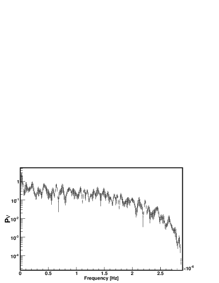
Figure 5: Measured power spectrum of PKS 1830-211, plotted in arbitrary units.

Figure 6: Double power spectrum of PKS 1830-211 plotted in arbitrary units. The solid line is a fit to a linear plus Gaussian profile.

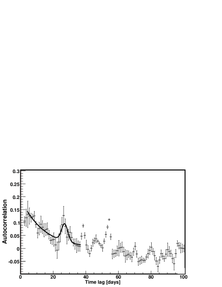
Figure 7: Measured autocorrelation function of PKS 1830-211. The solid line is a fit to an exponential plus Gaussian profile.

References

- Abdo et al. (2010) Abdo, A. A., Ackermann, M., Ajello, M., et al. 2010, VizieR Online Data Catalog, 218, 80405
- Atwood et al. (2009) Atwood, W. B., Abdo, A. A., Ackermann, M., et al. 2009, ApJ, 697, 1071
- Bogert et al. (1963) Bogert, B. P., Healy, M. J. R., & Tukey, J. W. 1963, in Proceedings on the Symposium on Time Series Analysis, ed. M.Rosenblat, Wiley, NY, 209–243
- Bolton et al. (2004) Bolton, A. S., Burles, S., Schlegel, D. J., Eisenstein, D. J., & Brinkmann, J. 2004, AJ, 127, 1860
- Brault & White (1971) Brault, J. W. & White, O. R. 1971, A&A, 13, 169
- Browne et al. (2003) Browne, I. W., Wilkinson, P. N., Jackson, N. J., et al. 2003, MNRAS, 341, 13
- Geiger & Schneider (1996) Geiger, B. & Schneider, P. 1996, MNRAS, 282, 530
- Jauncey et al. (1991) Jauncey, D. L., Reynolds, J. E., Tzioumis, A. K., et al. 1991, Nature, 352, 132
- Lidman et al. (1999) Lidman, C., Courbin, F., Meylan, G., et al. 1999, ApJ, 514, L57
- Lovell et al. (1998) Lovell, J. E. J., Jauncey, D. L., Reynolds, J. E., et al. 1998, ApJ, 508, L51
- Lovell et al. (1996) Lovell, J. E. J., Reynolds, J. E., Jauncey, D. L., et al. 1996, ApJ, 472, L5+
- Mattox et al. (1997) Mattox, J. R., Schachter, J., Molnar, L., Hartman, R. C., & Patnaik, A. R. 1997, ApJ, 481, 95
- Myers et al. (2003) Myers, S. T., Jackson, N. J., Browne, I. W. A., et al. 2003, MNRAS, 341, 1
- Pramesh Rao & Subrahmanyan (1988) Pramesh Rao, A. & Subrahmanyan, R. 1988, MNRAS, 231, 229
- Torres et al. (2003) Torres, D. F., Romero, G. E., Eiroa, E. F., Wambsganss, J., & Pessah, M. E. 2003, MNRAS, 339, 335
- Wiklind & Combes (1996) Wiklind, T. & Combes, F. 1996, in Astrophysics and Space Science Library, Vol. 206, Cold Gas at High Redshift, ed. M. N. Bremer & N. Malcolm, 227–+
- Winn et al. (2002) Winn, J. N., Kochanek, C. S., McLeod, B. A., et al. 2002, ApJ, 575, 103