Larkin-Ovchinnikov-Fulde-Ferrell Phase in (TMTSF)₂ClO₄ Superconductor: Theory versus Experiment

Abstract

We consider a formation of the Larkin-Ovchinnikov-Fulde-Ferrell (LOFF) phase in a quasi-one-dimensional (Q1D) conductor in a magnetic field, parallel to its conducting chains, where we take into account both the paramagnetic spin-splitting and orbital destructive effects against superconductivity. We show that, due to a relative weakness of the orbital effects in a Q1D case, the LOFF phase appears in (TMTSF)₂ClO₄ superconductor for real values of its Q1D band parameters. We compare our theoretical calculations with the recent experimental data by Y. Maeno’s group [S. Yonezawa et al., Phys. Rev. Lett. 100, 117002 (2008)] and show that there is a good qualitative and quantitative agreement between the theory and experimental data.

Since a discovery of superconductivity in organic (TMTSF)₂X conductors (X=PF₆ and ClO₄) [1], their physical properties have been intensively studied both experimentally and theoretically [2,3]. From the beginning, it was clear that their superconducting properties were unconventional. Indeed, it was found [4] that superconductivity was destroyed by non-magnetic impurities, which was recently unequivocally confirmed [5]. In addition, it was shown [6] that the conventional for s-wave superconductivity Hebel-Slichter peak was absent in the NMR experiments. Note that the experimental results [4-6] provide strong arguments that superconducting order parameter changes its sign on a quasi-one-dimensional (Q1D) Fermi surface (FS) of (TMTSF)₂X superconductors. On the other hand, they do not contain information about a spin-part of a superconducting order parameter and, thus, do not distinguish between singlet and triplet pairings. At the moment, the problem about a spin part of a superconducting order parameter in (TMTSF)₂X conductors is still controversial. Indeed, early measurements of the Knight shift in (TMTSF)₂PF₆ conductor [7] in a magnetic field $H=1.43\ T$ showed that spin susceptibility was unchanged through the superconducting transition. These data were interpreted as an evidence for triplet superconductivity. On the other hand, more recent Knight shift data in (TMTSF)₂ClO₄ conductor [8], obtained in a magnetic field $H=0.957\ T$, were interpreted in favor of a singlet superconducting pairing.

Another unconventional feature of superconductivity in (TMTSF)₂X conductors is very large upper critical fields for a magnetic field parallel to their conducting planes and perpendicular to their conducting chains, ${\bf H}\parallel{\bf b^{\prime}}$ [9-14]. These fields exceed both the quasi-classical orbital upper critical field [15,16] and so-called Clogston paramagnetic limit [17]. Note that in (TMTSF)₂PF₆ superconductor $H^{b^{\prime}}_{c2}$ is very large [10,11] due to a formation of domain walls in the vicinity of antiferromagnetic phase. In contrast, in (TMTSF)₂ClO₄ conductor large upper critical field $H^{b^{\prime}}_{c2}$ [12-14] is prescribed to $3D\rightarrow 2D$ dimensional crossover in a magnetic field, predicted in Ref.[18] and elaborated in Refs. [19-23]. In addition, recent measurements of the upper critical fields in (TMTSF)₂ClO₄ superconductor [13,14] have revealed another unusual property - a novel superconducting phase, which appears when a magnetic field is applied along the conducting chains, ${\bf H}\parallel{\bf a}$. It is shown [13,14] that the above mentioned phase is very sensitive to impurities and inclinations of a magnetic field from ${\bf a}$ axis. The authors of the experiments [13,14] have related this new phase with a possible formation of the Larkin-Ovchinnikov-Fulde-Ferrell (LOFF) state [24,25].

The goal of our Letter is to show theoretically that the LOFF phase has to appear in a magnetic field, parallel to the conducting chains of (TMTSF)₂ClO₄ superconductor, if we use experimentally measured values of its Q1D band parameters. The distinctive feature of our work is that we take into account both the paramagnetic spin-splitting and orbital destructive effects against superconductivity. This problem is a challenging one, since the orbital effects for a magnetic field along the conducting chains correspond to very particular open electron trajectories. These effects cannot be described by any of the existing theories, including Refs. [15-23,26]. To describe the orbital and paramagnetic effects, below we derive an integral equation for a superconducting order parameter, which, to the best of our knowledge, has not been considered before. By means of the measured Ginzburg-Landau slops of an anisotropic upper critical field in (TMTSF)₂ClO₄ [13,14] and the measured ratio $t_{a}/t_{b}$ [27,28], we determine its Q1D band parameters. We use these band parameters for a numerical solution of the above mentioned integral equation and conclude that the LOFF phase has to exist in (TMTSF)₂ClO₄ conductor. This conclusion is based both on theoretical arguments and on good qualitative and quantitative agreement between the theory and experimental measurements [13,14]. It is important that the results of our Letter support singlet d-wave scenario of superconductivity in (TMTSF)₂X materials.

Below, we consider a Q1D conductor with the following electron spectrum,

$$\epsilon({\bf p})=-2t_{a}\cos(p_{x}a/2)-2t_{b}\cos(p_{y}b^{*})-2t_{c}\cos(p_{z}c^{*}),$$ (1)

in a magnetic field, parallel to its conducting chains, ${\bf H}\parallel{\bf a}$,

$${\bf H}=(H,0,0),\ \ {\bf A}=(0,0,Hy),$$ (2)

where $t_{a}\gg t_{b}\gg t_{c}$ correspond to electron hoping integrals along ${\bf a}$ , ${\bf b}$, and ${\bf c}$ axes, respectively.

We represent electron wave functions with definite energy and momentum $p_{x}$ in the following way:

$$\Psi_{\epsilon}^{\pm}(p_{x};x,y)=\exp(\pm ip_{x}x)\exp[\pm ip^{\pm}_{y}(p_{x})y]\ \psi_{\epsilon}^{\pm}(p_{x},y),$$ (3)

where +(-) stands for left (right) sheet of a Q1D FS and the functions $p_{y}^{\pm}(p_{x})$ are defined by the equations:

$$v_{F}(p_{x}\mp p_{F})\mp 2t_{b}\cos[p^{\pm}_{y}(p_{x})b^{*}]=0,$$ (4)

where $v_{F}$ and $p_{F}$ are the Fermi velocity and Fermi momentum, respectively. In this case, we can rewrite Eq. (1) as:

$$\delta\epsilon^{\pm}({\bf p})=\pm 2t_{b}b^{*}(p_{y}-p_{y}^{\pm})\sin(p^{\pm}_{y}b^{*})-2t_{c}\cos(p_{z}c^{*}),$$ (5)

where we linearize the electron spectrum (1) near the FS with respect to momentum $p_{y}$; energy $\delta\epsilon=\epsilon-\epsilon_{F}$ is counted from the Fermi energy $\epsilon_{F}$.

In a magnetic field, we use the Peierls substitution method [18] for Eq.(5),

$$p_{y}-p^{\pm}_{y}\rightarrow-i\frac{d}{dy},\ p_{z}c^{*}\rightarrow p_{z}c^{*}-\frac{\omega_{c}}{v_{F}}y,\ \omega_{c}=\frac{eHv_{F}c^{*}}{c},$$ (6)

where $e$ is the electron charge and $c$ is the velocity of light. As a result, we obtain the following Schrodinger equation for the electron wave functions:

$$[\mp iv_{y}(p^{\pm}_{y})\frac{d}{dy} -2t_{c}\cos(p_{z}c^{*}-\frac{\omega_{c}}{v_{F}}y)-\mu_{B}\sigma H]\ \psi_{\epsilon}^{\pm}(p_{x},y,p_{z})$$ (7)

$$=\delta\epsilon\ \psi_{\epsilon}^{\pm}(p_{x},y,p_{z}),$$

with $\sigma/2$ being a projection of an electron spin on ${\bf a}$ axis; $\mu_{B}$ is the Bohr magneton, $v_{y}(p_{y})=2t_{b}b^{*}\sin(p_{y}b^{*})$.

It is important that Eq.(7) can be exactly solved:

$$\psi_{\epsilon}^{\pm}(p_{x},y,p_{z}) =\frac{1}{\sqrt{2\pi|v_{y}(p^{\pm}_{y})|}}\exp\biggl{[}\frac{\pm i\delta\epsilon y}{v_{y}(p^{\pm}_{y})}\biggl{]}\exp\biggl{[}\frac{\pm i\mu_{B}\sigma Hy}{v_{y}(p^{\pm}_{y})}\biggl{]}$$ (8)

$$\times\exp\biggl{[}\pm i\frac{2t_{c}}{v_{y}(p^{\pm}_{y})}\int^{y}_{0}\cos\biggl{(}p_{z}c^{*}-\frac{\omega_{c}}{v_{F}}u\biggl{)}du\biggl{]},$$

where the wave functions (8) are normalized by condition:

$$\int^{+\infty}_{-\infty}[\psi^{\pm}_{\epsilon_{1}}(p_{x},y,p_{z})]^{*}\ \psi^{\pm}_{\epsilon_{2}}(p_{x},y,p_{z})\ dy=\delta(\epsilon_{1}-\epsilon_{2}).$$ (9)

Note that finite temperature Green functions for the wave functions (8),(3) can be determined by the standard equation:

$$g_{i\omega_{n}}^{\pm}(x,x_{1};y,y_{1};p_{z})=\int^{+\infty}_{-\infty}d(\delta\epsilon)\frac{[\psi^{\pm}_{\epsilon}(x_{1},y_{1},p_{z})]^{*}\ \psi^{\pm}_{\epsilon}(x,y,p_{z})}{i\omega_{n}-\delta\epsilon},$$ (10)

where $\omega_{n}$ is the Matsubara frequency [29].

Below, we consider a singlet d-wave scenario of superconductivity in (TMTSF)₂ClO₄ conductor, which is in agreement with the experiments [4-6,8]. For this purpose we introduce the following d-wave like LOFF order parameter,

$$\Delta_{q}(x,y;p_{y})=\sqrt{2}\cos(p_{y}b^{*})\exp(iqx)\Delta_{q}(y),$$ (11)

where the Cooper pairs are characterized by non-zero total momentum along ${\bf a}$ axis, $q\neq 0$, and $\Delta_{q}(y)$ is the Ginzburg-Landau (GL) order parameter, which depends on coordinate $y$. To derive the gap equation for $\Delta_{q}(y)$, we use the Gor’kov equations for non-uniform superconductivity [30,31], as it is done, for example, in Ref.[32]. As a result of lengthy but rather straightforward calculations, we obtain:

$$\Delta_{q}(y)=g\int\frac{dp_{y}}{v_{x}(p_{y})}\int_{|y-y_{1}|>\frac{|v_{y}|}{\Omega}}\frac{2\pi Tdy_{1}}{v_{y}(p_{y})\sinh\bigl{[}\frac{2\pi T|y-y_{1}|}{v_{y}(p_{y})}\bigl{]}}$$

$$\times 2\cos^{2}(p_{y}b^{*})\cos\biggl{[}\frac{2\beta\mu_{B}H(y-y_{1})}{v_{y}(p_{y})}\biggl{]}\ \cos\biggl{[}q\frac{v_{x}(p_{y})}{v_{y}(p_{y})}(y-y_{1})\biggl{]}$$

$$\times J_{0}\biggl{\{}\frac{8t_{c}v_{F}}{\omega_{c}v_{y}(p_{y})}\sin\biggl{[}\frac{\omega_{c}(y-y_{1})}{2v_{F}}\bigg{]}\sin\biggl{[}\frac{\omega_{c}(y+y_{1})}{2v_{F}}\bigg{]}\biggl{\}}\Delta_{q}(y_{1}),$$ (12)

where factor $\beta$ takes into account possible decrease of the spin-splitting paramagnetic effects due to small deviations from a weak coupling scenario; $g$ is an effective electron coupling constant, $\Omega$ is a cutoff energy. Note that the last term in Eq.(12) describes the orbital effects against superconducting at low enough magnetic fields. At high magnetic fields, quantum effects due to the Bragg reflections of electrons from boundaries of the Brillouin zone, as shown in Refs. [18,32], can improve superconductivity. This improvement may cause to the appearance of the Reentrant Superconducting (RS) phase [18-23,32]. Our analysis of Eq.(12) shows that the RS phase may appear only at magnetic fields of the order of $50\ T$, where superconductivity is already destroyed by the paramagnetic spin-splitting effects. Therefore, for a magnetic field parallel to the conducting axis, ${\bf H}\parallel{\bf a}$, unlike the situation, where it is perpendicular to it, ${\bf H}\parallel{\bf b^{\prime}}$ [18-23], we can ignore the above mentioned RS effects. From mathematical point of view, this means that we can replace the term $\sin[\frac{\omega_{c}(y-y_{1})}{2v_{F}}]\sin[\frac{\omega_{c}(y+y_{1})}{2v_{F}}]$ by $\frac{\omega^{2}_{c}(y^{2}-y^{2}_{1})}{4v^{2}_{F}}$ in Eq.(12). If we do this and if we introduce more convenient variables, $y=y$, $y_{1}=y+\frac{v_{y}(p_{y})}{v_{F}}z$, we can rewrite Eq.(12) as:

$$\Delta_{q}(y)=g\int\frac{dp_{y}}{v_{x}(p_{y})}\int_{|z|>\frac{v_{F}}{\Omega}}\frac{2\pi Tdz}{v_{F}\sinh\bigl{[}\frac{2\pi Tz}{v_{F}}\bigl{]}}$$

$$\times 2\cos^{2}(p_{y}b^{*})\cos\biggl{[}\frac{2\beta\mu_{B}Hz}{v_{F}}\biggl{]}\ \cos\biggl{[}q\frac{v_{x}(p_{y})}{v_{F}}z\biggl{]}$$

$$\times J_{0}\biggl{\{}\frac{2t_{c}eHc^{*}}{v_{F}c}z\biggl{[}2y+\frac{v_{y}(p_{y})}{v_{F}}z\biggl{]}\biggl{\}}\ \Delta_{q}\biggl{[}y+\frac{v_{y}(p_{y})}{v_{F}}z\biggl{]}.$$ (13)

It is possible to show that in the vicinity of transition temperature, $(T_{c}-T)\ll T_{c}$, Eq.(13) is equivalent to the GL expression for the upper critical field,

$$H^{a}_{c2}=\frac{4\sqrt{2}\pi^{2}c\hbar T^{2}_{c}}{7\zeta(3)et_{b}t_{c}b^{*}c^{*}}\biggl{(}\frac{T_{c}-T}{T_{c}}\biggl{)},$$ (14)

where $\zeta(x)$ is the Riemann zeta function.

Let us briefly discuss how to determine band parameters $t_{a},t_{b}$, and $t_{c}$ from analysis of the available experimental data in (TMTSF)₂ClO₄ conductor [33]. First of all, the ratio $t_{a}/t_{b}\simeq 10$ was firmly established in Ref.[28], where the measured Lee-Naughton-Lebed oscillations were compared with the corresponding theoretical results. Second, in Refs.[13,14], the GL slopes for the upper critical fields along ${\bf b}$ and ${\bf c}$ axes were carefully measured: $dH^{b}_{c2}/dT=2.75\ T/K$ and $dH^{c}_{c2}/dT=0.14\ T/K$. If we take into account that for d-wave like order parameter (11) in the GL region [33]:

$$H^{b}_{c2}=\frac{8\pi^{2}c\hbar T^{2}_{c}}{7\zeta(3)et_{a}t_{c}ac^{*}}\biggl{(}\frac{T_{c}-T}{T_{c}}\biggl{)}$$ (15)

and

$$H^{c}_{c2}=\frac{8\sqrt{2}\pi^{2}c\hbar T^{2}_{c}}{7\zeta(3)et_{a}t_{b}ab^{*}}\biggl{(}\frac{T_{c}-T}{T_{c}}\biggl{)},$$ (16)

then we can evaluate all three band parameters: $t_{a}=1340\ K$, $t_{b}=134\ K$, $t_{c}=2.6\ K$. In Eqs.(15),(16), we use the following known values: $T_{c}=1.45\ K$, $a=7.1\ \AA$, $b^{*}=7.2\ \AA$, and $c^{*}=13.1\ \AA$ [13,14].

In Fig.(1), we compare the result of numerical solutions of Eq.(13) for $\beta=0.9$ with the experimental data [13] and predict the appearance of the LOFF phase at $H\geq 3\ T$ (see also the figure caption). Note that the only fitting parameter in our theory is $\beta$. We interpret the above mentioned value $\beta=0.9$, which fits better the experimental data [13], as an evidence of small deviations from a weak coupling scenario of superconductivity, where $\beta=1$.

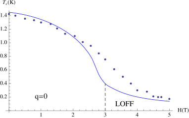
Figure 1: Numerical solution of Eq.(13) (solid line) is compared to the experimental data [13] (dottes). Note that a phase transition from uniform superconductivity (q=0) to the Larkin-Ovchinnikov-Felde-Ferrell phase ($q\neq 0$) is predicted by our theory in a magnetic field $H\simeq 3\ T$. We pay attention on a good overall qualitative and quantitative agreement between the theory and experiment.

Here, we summarize the main results of the Letter. We have derived an integral equation, which allows to describe superconductivity in a magnetic field, parallel to conducting axes of a Q1D conductor. By using numerical solutions of the above mentioned equation for experimentally measured band parameters of (TMTSF)₂ClO₄ compound, we have found that the LOFF phase has to appear in this superconductor at high enough magnetic fields. Comparison of our theoretical curve with the recent experimental data [13] demonstrates a good overall qualitative and quantitative agreement (see Fig.1).

For theoretical discussions of a possibility of the appearance of the LOFF phase in a Q1D conductor in a magnetic field, perpendicular to conducting axes and parallel to conducting planes, see Refs.[18,20-23]. There are some experimental data in a favor of the existence of the LOFF phase in quasi-two-dimensional (Q2D) superconductors $\kappa$-(ET)₂Cu(NCS)₂ [34,35], $\lambda$-(BETS)₂GaCl₄ [36], and $\lambda$-(BETS)₂FeCl₄ [37]. Nevertheless, theoretical calculations, which take into account both the orbital and paramagnetic effects in a Q2D case, have not been done yet . The paramagnetic spin-splitting effects in the LOFF phase in a pure 1D case were theoretically studied in Ref. [38], whereas they were theoretically studied in a pure 2D case in a number of papers [39-43].

One of us (A.G.L.) is thankful to N.N. Bagmet (Lebed) for very useful discussions. This work was supported by the NSF under Grant No DMR-0705986.

^∗Also at: Landau Institute for Theoretical Physics, 2 Kosygina Street, Moscow, Russia.

References

- (1) D. Jerome, A. Mazaud, M. Ribault, and K. Bechgaard, J. Phys. (Paris) Lett. 41, L95 (1980).
- (2) The Physics of Organic Superconductors and Conductors, edited by A.G. Lebed (Springer, Berlin, 2008).
- (3) T. Ishiguro, K. Yamaji, and G. Saito, Organic Superconductors, 2nd ed. (Springer, Berlin, 1998).
- (4) See, for example, M.-Y. Choi, P.M. Chaikin, S.Z. Huang, P. Haen, E.M. Engler, and R.L. Greene, Phys. Rev. B 25, 6208 (1982).
- (5) N. Joo, P. Auban-Senzier, C.R. Pasquier, D. Jerome, and K. Bechgaard, Europhys. Lett. 72, 645 (2005).
- (6) M. Takigawa, H. Yasuoka, and G. Saito, J. Phys. Soc. Jpn. 56, 873 (1987).
- (7) I.J. Lee, S.E. Brown, W.G. Clark, M.J. Strouse, M.J. Naughton, W. Kang, and P.M. Chaikin, Phys. Rev. Lett. 88, 017004 (2002).
- (8) J. Shinagawa, Y. Kurosaki, F. Zhang, C. Parker, S.E. Brown, D. Jerome, J.B. Christensen, and K. Bechgaard, Phys. Rev. Lett. 98, 147002 (2007).
- (9) I.J. Lee, M.J. Naughton, G.M. Danner, and P.M. Chaikin, Phys. Rev. Lett. 78, 3555 (1997).
- (10) I.J. Lee, P.M. Chaikin, and M.J. Naughton, Phys. Rev. B 62, R14669 (2000).
- (11) I.J. Lee, P.M. Chaikin, and M.J. Naughton, Phys. Rev. B 65, 180502(R) (2002).
- (12) J.I. Oh and M.J. Naughton, Phys. Rev. Lett. 92, 067001 (2004).
- (13) S. Yonezawa, S. Kusaba, Y. Maeno, P. Auban-Senzier, C. Pasquier, K. Bechgaard, and D. Jerome, Phys. Rev. Lett. 100, 117002 (2008).
- (14) S. Yonezawa, S. Kusaba, Y. Maeno, P. Auban-Senzier, C. Pasquier, and D. Jerome, Journal of Physics: Conference Series 150, 052289 (2009).
- (15) L.P. Gor’kov, Zh. Eksp. Teor. Fiz. 37, 833 (1959) [Sov. Phys. JETP 10, 593 (1960)].
- (16) N.R. Werthamer, E. Helfand, and P.C. Hohenberg, Phys. Rev. 147, 295 (1966).
- (17) A.M. Clogston, Phys. Rev. Lett. 9, 266 (1962); B.S. Chandrasekhar, Appl. Phys. Lett. 1, 7 (1962).
- (18) A.G. Lebed, JETP Lett. 44, 114 (1986) [Pis’ma Zh. Eksp. Teor. Fiz. 44, 89 (1986)].
- (19) L.I. Burlachkov, L.P. Gor’kov, and A.G. Lebed, Europhys. Lett. 4, 941 (1987).
- (20) N. Dupuis, G. Montambaux, and C.A.R. Sa de Melo, Phys. Rev. Lett. 70, 2613 (1993); N. Dupuis and G. Montambaux, Phys. Rev. B. 49, 8993 (1994).
- (21) C. A. R. Sa de Melo, Physica C 260, 224 (1996).
- (22) Y. Hasegawa and M. Miyazaki, J. Phys. Soc. Jpn. 65, 1028 (1996); M. Miyazaki and Y. Hasegawa, ibid. 65, 3283 (1996).
- (23) N. Belmechri, G. Abramovici and M. Heritier, Europhys. Lett. 82, 47009 (2008).
- (24) A.I. Larkin and Yu.N. Ovchinnikov, Zh. Eksp. Teor. Phys. 47, 1136 (1964) [Sov. Phys. JETP 20, 762 (1965)].
- (25) P. Fulde and R.A. Ferrell, Phys. Rev. 135, A550 (1964).
- (26) H. Won, K. Maki, S. Haas, N. Oeschler, F. Weickert, and P. Gegenwart, Phys. Rev. B 69, 180504(R) (2004).
- (27) A.G. Lebed and M.J. Naughton, Phys. Rev. Lett. 91, 187003 (2003).
- (28) A.G. Lebed, Heon-Ick Ha, and M.J. Naughton, Phys. Rev. B 71, 132504 (2005).
- (29) A.A. Abrikosov, L.P. Gor’kov, and I.E. Dzyaloshinski, Methods of Quantum Field Theory in Statistical Physics (Dover, New York, 1975).
- (30) V.P. Mineev and K.V. Samokhin, Introduction to Unconventional Superconductivity (Gordon and Breach, Amsterdam, 1999).
- (31) M. Sigrist and K. Ueda, Rev. Mod. Phys. 63, 239 (1991).
- (32) A.G. Lebed and K. Yamaji, Phys. Rev. Lett. 80, 2697 (1998).
- (33) For a detail derivation of the Ginzburg-Landau slopes in a Q1D conductor and for determination of the band parameters in (TMTSF)2X materials, see A.G. Lebed, Phys. Rev. B, submitted.
- (34) R. Lortz, Y. Wang, A. Demuer, P.H.M. Bottger, B. Bergk, G. Zwicknagl, Y. Nakazawa, and J. Wosnitza, Phys. Rev. Lett. 99, 187002 (2007).
- (35) J. Singleton, J.A. Symington, M.-S. Nam, A. Ardavan, M. Kurmoo, and P. Day, J. Phys. Condens. Matt. 12, L641 (2000).
- (36) M.A. Tanatar, T. Ishiguro, H. Tanaka, and H. Kobayashi, Phys. Rev. B 66, 134503 (2002).
- (37) L. Balikas, J.S. Brooks, K. Storr, S. Uji, M. Tokumoto, H. Tanaka, H. Kobayashi, A. Kobayashi, V. Barzykin, and L.P. Gor’kov, Phys. Rev. Lett. 87, 067002 (2001).
- (38) A.I. Buzdin and V.V. Tugushev, Zh. Eksp. Teor. Phys. 85, 735 (1983) [Sov. Phys. JETP 58, 428 (1983)].
- (39) L.N. Bulaevskii, Zh. Eksp. Teor. Fiz. 65, 1278 (1973) [Sov. Phys. JETP 38, 634 (1974)].
- (40) H. Shimahara, J. Phys. Soc. Jpn. 67, 736 (1998).
- (41) H. Shimahara, J. Phys. Soc. Jpn. 71, 1644 (2002).
- (42) M. Houzet, A. Buzdin, L. Bulaevskii, M. Maley, Phys. Rev. Lett. 88, 227001 (2002).
- (43) Z. Zheng and D.F. Agterberg, Phys. Rev. B 82, 024506 (2010).