Control-free control: manipulating a quantum system using only a limited set of measurements

Abstract

We present and discuss different protocols for preparing an arbitrary quantum state of a qubit using only a restricted set of measurements, with no unitary operations at all. We show that an arbitrary state can indeed be prepared, provided that the available measurements satisfy certain requirements. Our results shed light on the role that measurement-induced back-action plays in quantum feedback control and the extent to which this back-action can be exploited in quantum-control protocols.

I Introduction

Control techniques are applied in a wide variety of practical applications, e.g. when a device is to be maintained in a certain state in spite of the environmental fluctuations that would normally push it away from that state ControlSystemBook . The basic structure of a closed-loop control system contains two steps: measurement and feedback control. In the first step, i.e. the measurement, information is acquired about the state of the system and how far it is from the desired target state. In the second step, a “control” is applied to the system, i.e. a signal or force is applied, in order to change the state of the system and guide it towards the target state.

In classical mechanics, the measurement process only extracts information about the state of the system, but (under ideal circumstances) it does not change that state. In quantum mechanics, this picture breaks down: the measurement itself will change the state of the system no matter how ideal it is (Note that for any measurement outcome there are quantum states that are not affected by the measurement; this absence of back-action, however, cannot be true for a general state). One therefore needs to treat quantum-control problems using a different frame of mind from that used when dealing with classical-control problems WisemanBook ; Brif ; Peirce .

One possibility for dealing with the unavoidable back-action of the measurement is to calculate the effected change and design the control signal accordingly Belavkin ; Wiseman . Another possibility, which might be conceptually more radical, is to use the change caused by the measurement as the sole means for manipulating the state of the system. In this case, closed-loop feedback control involves only the measurement step; the “control” is no longer needed. Indeed there have been some studies on this possibility in the past few years Roa ; Pechen ; Jacobs .

In previous work Roa ; Pechen ; Jacobs it was assumed that measurements in any basis are allowed. Here we consider the case where only a restricted set of measurements is implementable, and we analyze various questions related to whether such a limited set of operations is sufficient for the preparation of an arbitrary target state. We also consider the question of the time required to reach the desired target state.

II State preparation using the full set of possible measurements

In Refs. Roa ; Pechen the authors considered the problem of preparing an arbitrary target state from an arbitrary initial state without imposing any constraints on the measurements that can be performed on the system. There it was demonstrated that an arbitrary target state can indeed be prepared using only measurements. One can understand this situation as follows. For any target state $\left|\psi_{T}\right\rangle$, one can construct (at least formally) a projective measurement where $\left|\psi_{T}\right\rangle$ is one of the possible outcomes. If now the above-described measurement is performed on a system in any initial state, there is a possibility that the outcome will correspond to the state $\left|\psi_{T}\right\rangle$, and one would have succeeded in preparing the target state. This procedure is obviously probabilistic; it is possible that one might obtain a different outcome in the measurement. Turning this probabilistic protocol into a deterministic one is straightforward: every time the measurement fails to produce the desired outcome, a perturbation, which can be thought of as a kick, can be applied to the system and the measurement is repeated. Unless the perturbation does not create any population in the state $\left|\psi_{T}\right\rangle$, e.g. for symmetry reasons, this procedure is deterministic; if one keeps trying, one will eventually obtain the target state Hida .

In an increasingly large Hilbert space, it becomes more and more unlikely to obtain the desired measurement outcome, which in turn leads to longer and longer average state-preparation times. This problem can be alleviated by making a better choice of measurements than the one described above. One can guide the quantum state of the system from the initial state to the target state using a sequence of projective measurements where one of the possible outcomes gradually changes from the initial state $\left|\psi_{I}\right\rangle$ to the target state $\left|\psi_{T}\right\rangle$. For example, one could design a sequence of $N$ projective measurements where each measurement (labelled by the index $i$) has one outcome that corresponds to the projection $\left|\psi_{i}\right\rangle\left\langle\psi_{i}\right|$, where

$$\left|\psi_{i}\right\rangle=\cos\left(\frac{\pi i}{2N}\right)\left|\psi_{I}\right\rangle+\sin\left(\frac{\pi i}{2N}\right)\left|\psi_{T}\right\rangle.$$ (1)

For best performance, we assume that the other outcomes of the measurement are orthogonal to $\left|\psi_{i}\right\rangle$. The probability that the system will follow the state $\left|\psi_{i}\right\rangle$ in all the measurement steps is given by $\cos^{2N}\left[\pi/(2N)\right]$, which approaches unity in the limit $N\rightarrow\infty$, regardless of the size of the Hilbert space. This procedure was analyzed in Refs. Roa ; Pechen ; vonNeumann .

In Ref. Jacobs the author considered the case of continuous measurement, where one essentially performs weak measurements rather than projective measurements. There it was demonstrated that by continuously adjusting the measurement settings, an arbitrary target state can be prepared. The choice of the measurement is done as follows: based on the instantaneous quantum state and the desired target state, one chooses a measurement basis that gives a high probability for the quantum state to evolve towards the target state.

III State preparation using a restricted set of measurements

In the previous section, we reviewed a number of ideas that can be used for the preparation of an arbitrary target state using the set of all possible measurements as available resources. In the following, we consider the possibility of preparing an arbitrary target state using a small number of available measurements. Indeed, in realistic situations there typically are constraints on the measurements that can be performed.

III.1 Measurements of spin along three orthogonal axes

We consider a two-level system, i.e. a qubit, and we start by considering measurements of this (pseudo-)spin along three orthogonal axes, i.e. the observables $\sigma_{x,y,z}$. If the measurements were projective, the $\sigma_{x}$ measurement would result in one of the states $\left|\sigma_{x}=1\right\rangle$ and $\left|\sigma_{x}=-1\right\rangle$, depending on the outcome of the measurement, and similarly for the two other observables. As a result, only six target states can be prepared: $\left|\sigma_{x}=1\right\rangle$, $\left|\sigma_{x}=-1\right\rangle$, $\left|\sigma_{y}=1\right\rangle$, $\left|\sigma_{y}=-1\right\rangle$, $\left|\sigma_{z}=1\right\rangle$ and $\left|\sigma_{z}=-1\right\rangle$ (Below, we shall use the notation $\left|\uparrow\right\rangle=\left|\sigma_{z}=1\right\rangle$ and $\left|\downarrow\right\rangle=\left|\sigma_{z}=-1\right\rangle$).

Figure 1: (Color online) Schematic diagram showing the transformation of the quantum state of a qubit as a result of a non-projective measurement. The double arrow represents the measurement axis. The tail of the single-headed arrow represents the pre-measurement state, and the head represents the post-measurement state. The quantum state “moves” in the plane defined by the pre-measurement state and the measurement axis. The distance that the quantum state moves depends on the different parameters in the problem, including in particular the measurement strength $\epsilon$.

The situation changes drastically when, instead of strong projective measurements, we consider weak, non-projective measurements. An example of a weak measurement could be the following: A measurement of $\sigma_{z}$ produces the outcome $+1$ or $-1$, upon which the quantum state of the system is transformed (or, in some sense, partially projected) according to the formula

$$\rho_{\rm after}=\frac{\hat{M}_{\pm}\rho_{\rm before}\hat{M}_{\pm}}{{\rm Tr}\{\hat{M}_{\pm}\rho_{\rm before}\hat{M}_{\pm}\}},$$ (2)

where the measurement operators $\hat{M}_{\pm}$ are given by

$$\hat{M}_{+} = \sqrt{\frac{1+\epsilon}{2}}\left|\uparrow\right\rangle\left\langle\uparrow\right|+\sqrt{\frac{1-\epsilon}{2}}\left|\downarrow\right\rangle\left\langle\downarrow\right|$$

$$\hat{M}_{-} = \sqrt{\frac{1-\epsilon}{2}}\left|\uparrow\right\rangle\left\langle\uparrow\right|+\sqrt{\frac{1+\epsilon}{2}}\left|\downarrow\right\rangle\left\langle\downarrow\right|,$$ (3)

and the probability of observing the two different outcomes are given by

$${\rm Prob}_{\pm}={\rm Tr}\{\hat{M}_{\pm}\rho_{\rm before}\hat{M}_{\pm}\}.$$ (4)

The parameter $\epsilon$ quantifies the strength of the measurement: for a weak measurement $\epsilon$ is small, whereas for a projective measurement $\epsilon=1$ (The parameter $\epsilon$ can also be understood as the measurement fidelity Ashhab ). We shall assume similar measurement properties for the two other observables. A weak $\sigma_{z}$ measurement does not project the system onto one of the two states $\left|\uparrow\right\rangle$ and $\left|\downarrow\right\rangle$, but rather slightly modifies the quantum state such that it experiences a small shift from the pre-measurement state in the direction of one of the states $\left|\uparrow\right\rangle$ and $\left|\downarrow\right\rangle$. For example, if one starts with the state

$$\left|\psi\right\rangle_{\rm before} = \frac{1}{\sqrt{2}}\left(\left|\uparrow\right\rangle+\left|\downarrow\right\rangle\right)$$ (5)

$$= 0.707\left|\uparrow\right\rangle+0.707\left|\downarrow\right\rangle,$$

and one obtains the outcome $+1$ in a $\sigma_{z}$ measurement of strength $\epsilon=0.01$, the post-measurement state will be (approximately)

$$\left|\psi\right\rangle_{\rm after}=0.711\left|\uparrow\right\rangle+0.703\left|\downarrow\right\rangle.$$ (6)

The transformation of the quantum state of a qubit following a non-projective measurement is illustrated in Fig. 1.

One can now observe that after a weak measurement of a given observable, the post-measurement state lies in the plane defined by the pre-measurement state and the measurement axis. Using this observation, one can devise a protocol for preparing an arbitrary target state using the three measurements mentioned above. One possibility is the following: One performs a sequence of $\sigma_{x}$ and $\sigma_{y}$ measurements until the quantum state of the system lies in the plane defined by the $z$-axis and the target state. Once that goal is achieved, one performs a $\sigma_{z}$ measurement (or measurements), such that one either obtains the target state or one concludes that the state has gone too far in the opposite direction and is unlikely to come back (clearly the above is a subjective explanation; however, it can be made quantitative straightforwardly, as we shall do shortly). As a general rule, one could say that success and failure in this (i.e. second) step occur with probability 50% each. In the case of failure, one goes back to the $\sigma_{x}$ and $\sigma_{y}$ measurements. This time one requires again that the state lie in the plane defined by the $z$-axis and the target state, but one also requires that the state approach the $x$-$y$ plane to within a certain tolerance (this new condition is designed to bring the state back to roughly the middle between the states $\left|\uparrow\right\rangle$ and $\left|\downarrow\right\rangle$, such that the next attempt at a $\sigma_{z}$ measurement will have a 50% success probability).

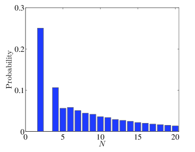
Figure 2: (Color online) The probability of obtaining the target state $\left|\psi_{T}\right\rangle=\cos\frac{\pi}{8}e^{-i\pi/8}\left|\uparrow\right\rangle+\sin\frac{\pi}{8}e^{i\pi/8}\left|\downarrow\right\rangle$ in $N$ measurement steps starting from the initial state $\left|\psi_{I}\right\rangle=(e^{-i\pi/4}\left|\uparrow\right\rangle+e^{i\pi/4}\left|\downarrow\right\rangle)/\sqrt{2}$ and following the procedure explained in Sec. III.A. For this particular choice of states, the average number of measurement steps is 10.5 and the probability of successful state preparation in under twenty steps is 0.86.

We now estimate the time required in order to prepare an arbitrary quantum state using the above protocol. For this purpose we assume that the measurement fidelity $F$ in a single measurement is a tunable parameter (If one is constrained to use measurements of a small fidelity $\epsilon$, any larger fidelity $F$ can be obtained by repeating the low-fidelity measurement $n$ times with $n$ given by

$$F={\rm erf}[\epsilon\sqrt{n\pi}/2]\approx 1-\exp\{-n\epsilon\},$$ (7)

and ${\rm erf}$ stands for the error function Ashhab ). The target state can be expressed as

$$\left|\psi_{T}\right\rangle=\cos\frac{\theta_{T}}{2}e^{-i\phi_{T}/2}\left|\uparrow\right\rangle+\sin\frac{\theta_{T}}{2}e^{i\phi_{T}/2}\left|\downarrow\right\rangle,$$ (8)

up to an irrelevant overall phase. For definiteness we assume that the initial state points along the $y$-axis, i.e. the initial state is an eigenstate of $\hat{\sigma}_{y}$. As explained above, before performing any $\sigma_{z}$ measurements, one first needs to prepare the state

$$\left|\psi\right\rangle=\frac{1}{\sqrt{2}}\left(e^{-i\phi_{T}/2}\left|\uparrow\right\rangle+e^{i\phi_{T}/2}\left|\downarrow\right\rangle\right).$$ (9)

A measurement of $\sigma_{x}$ with fidelity $F=|\cos\phi_{T}|$ results in the desired state with probability 0.5. In the case of failure, a strong (and ideally projective) $\sigma_{y}$ measurement is performed, followed by a new attempt using the $\sigma_{x}$ measurement (One should note here that the strong $\sigma_{y}$ measurement could result in a state with a value of $\phi$ that differs from $\phi_{T}$ by more than $\pi/2$. In this case, it is impossible for any $\sigma_{x}$ measurement to produce the desired value of $\phi$. One could deal with this case by performing a strong $\sigma_{x}$ measurement, followed by a $\sigma_{y}$ measurement with a properly calibrated fidelity). One can therefore estimate that obtaining a state with the desired value of the phase $\phi_{T}$ will, on average, require just a few measurement steps. We now have a state that lies in the $x$-$y$ plane with the correct phase between the states $\left|\uparrow\right\rangle$ and $\left|\downarrow\right\rangle$. At this point, a $\sigma_{z}$ measurement with fidelity $F=|\cos\theta_{T}|$ results in the target state with probability 0.5. In other words, every time one succeeds in obtaining the desired value of $\phi_{T}$, one has a 50% chance of obtaining $\left|\psi_{T}\right\rangle$ in the ensuing $\sigma_{z}$ measurement. In the case where the $\sigma_{z}$ measurement fails to produce the target state, one performs a strong $\sigma_{y}$ measurement and goes back to the first step of the procedure explained above. Since each attempt at preparing the target state involves a few measurements (roughly three to five), and each attempt has a success probability of 0.5, one can conclude that one has a high probability of preparing the target state $\left|\psi_{T}\right\rangle$ in under twenty measurement steps. In Fig. 2 we plot the probability histogram for the number of measurement steps required to prepare the target state $\left|\psi_{T}\right\rangle=\cos\frac{\pi}{8}e^{-i\pi/8}\left|\uparrow\right\rangle+\sin\frac{\pi}{8}e^{i\pi/8}\left|\downarrow\right\rangle$ starting from the initial state $\left|\psi_{I}\right\rangle=(e^{-i\pi/4}\left|\uparrow\right\rangle+e^{i\pi/4}\left|\downarrow\right\rangle)/\sqrt{2}$.

III.2 Single measurement setting: symmetric, informationally complete, positive operator valued measure

Another interesting setup to consider is that of a qubit measured using a symmetric, informationally complete, positive operator valued measure (SIC-POVM). The reason why informationally complete POVMs are interesting in this context is that they can (partially) project the state of the system towards one of four different directions that span the entire Bloch sphere, giving the quantum state the possibility of moving in all directions about the Bloch sphere.

The SIC-POVM on a single qubit is a measurement with four possible outcomes where the four different outcomes correspond to quantum states that form a tetrahedon on the Bloch sphere. One representative choice of a SIC-POVM, which is equivalent to any other SIC-POVM of the same strength up a rotation, is the one with the following measurement operators:

$$\hat{M}_{i}=\frac{\sqrt{1+\epsilon}}{2}\left|\psi_{i}\right\rangle\left\langle\psi_{i}\right|+\frac{\sqrt{1-\epsilon}}{2}\left|\overline{\psi}_{i}\right\rangle\left\langle\overline{\psi}_{i}\right|$$ (10)

with

$$\left|\psi_{1}\right\rangle = \left|\uparrow\right\rangle$$

$$\left|\psi_{2}\right\rangle = \sqrt{\frac{1}{3}}\left|\uparrow\right\rangle+\sqrt{\frac{2}{3}}\left|\downarrow\right\rangle$$

$$\left|\psi_{3}\right\rangle = \sqrt{\frac{1}{3}}\left|\uparrow\right\rangle+\sqrt{\frac{2}{3}}e^{2i\pi/3}\left|\downarrow\right\rangle$$

$$\left|\psi_{4}\right\rangle = \sqrt{\frac{1}{3}}\left|\uparrow\right\rangle+\sqrt{\frac{2}{3}}e^{-2i\pi/3}\left|\downarrow\right\rangle,$$ (11)

where $\left|\overline{\psi}_{i}\right\rangle$ represents the quantum state orthogonal to $\left|\psi_{i}\right\rangle$, and $\epsilon$ quantifies the strength of the measurement.

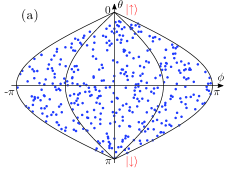
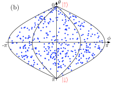
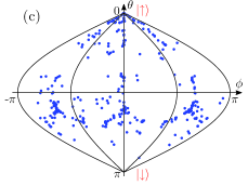
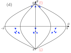
Figure 3: (Color online) The distribution of states obtained from repeated measurement using a SIC-POVM. The different panels correspond to different measurement strengths: $\epsilon=0.1$ (a), 0.5 (b), 0.9 (c) and 0.99 (d). In each panel 400 point are plotted. Each point represents the values of the spherical coordinates $\theta$ and $\phi$ of the quantum state $\left|\psi\right\rangle$, plotted using a map-like scheme designed not to distort the areas of different regions on the surface of the Bloch sphere. In order to obtain a distribution that is representative of the long-time steady state, each simulation involves a sequence of $10^{5}$ measurement steps. The 400 points in each panel represent the quantum state at equally spaced measurement steps, i.e. we plot the coordinates of the state after measurement step number 250, 500, 750, … The results shown in this figure are independent of the initial state used in the calculations.

In Fig. 3 we plot the coordinates of a quantum state that is repeatedly measured using the SIC-POVM given above. If one consider the case $\epsilon=1$ (not plotted), only the four states $\left|\psi_{1}\right\rangle$, $\left|\psi_{2}\right\rangle$, $\left|\psi_{3}\right\rangle$, $\left|\psi_{4}\right\rangle$ are realized as post-measurement states. It should be noted here that (unlike von-Neumann measurements) even if the state is one of these four states at a given step, repeated measurement will not necessarily produce the same outcome; it is possible that in the next step a different outcome is obtained, and the state of the system changes to the corresponding state. As can be seen clearly from Fig. 3(d), for values of $\epsilon$ that are close to one, e.g. at $\epsilon=0.99$, there are 16 possible states that appear as a result of the repeated measurements: the original four states (i.e. the ones that appear for $\epsilon=1$), and three more states surrounding each one of the original four states. These four sets of three additional states correspond to obtaining the outcome $i$ given that the state was (approximately) given by $\left|\psi_{j}\right\rangle$ in the previous step (with all the different combinations of $i,j=1,2,3,4$). When $\epsilon$ is reduced to 0.9 [Fig. 3(c)], the sixteen-point structure cannot be seen anymore, but we can clearly identify that the points are concentrated in four regions on the surface of the Bloch sphere. When $\epsilon$ is reduced to 0.5 or below, we can see that the states now cover the entire Bloch sphere, such that any state can be prepared CommentRegardingFiniteEpsilon . The reason why the states are no longer concentrated around the four outcome states is that for small values of $\epsilon$ the projection in each measurement step is only partial, and the state undergoes a rather stochastic motion on the Bloch sphere, allowing it to access all regions on the surface of the Bloch sphere. It should be emphasized here that even though the motion of the state is stochastic, one can keep track of this motion given the record of the outcomes that have been obtained in the sequence of measurements. One is therefore able to tell if the state hits the target state $\left|\psi_{T}\right\rangle$ (up to the accepted tolerance level). It is therefor possible to prepare any target state $\left|\psi_{T}\right\rangle$ by repeatedly performing measurements using a single SIC-POVM, provided that $\epsilon<1$.

One can obtain a quick estimate for the time required to prepare an arbitrary target state by assuming that the state after each measurement step is randomly located on the Bloch sphere, independently of the measurement history. If the error tolerance is set such that a deviation by an angle smaller than $\delta$ is accepted, then one can divide the solid angle of the entire Bloch sphere, i.e. $4\pi$, by the solid angle defined by the deviation $\delta$, i.e. $\pi\delta^{2}$. The resulting estimate is that it would take on average $4/\delta^{2}$ steps in order to prepare an arbitrary target state.

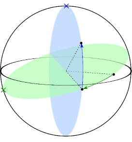
Figure 4: (Color online) Schematic diagram showing how a given initial state can be transformed into a given target state after two applications of the SIC-POVM with appropriately chosen measurement strengths. The first measurement brings the quantum state into the plane defined by the target state and one of the SIC-POVM states $\left|\psi_{i}\right\rangle$, and the second measurement results in the target state. It should be emphasized that the success of each one of these two steps is probabilistic.

The above estimate for the average preparation time assumed weak measurements. Alternatively one could assume a tunable measurement strength in order to speed up the state-preparation process. We have used numerical calculations to verify the following statement: Given any initial state, it is possible to end up in any given target state after at most three measurements, provided that the measurement strengths are tuned properly and one obtains the correct measurement outcomes. A typical example, where only two steps are needed, is illustrated in Fig. 4. One can therefore conclude that it should be possible to prepare any desired target state with high probability in under twenty measurement steps. We shall not go into any detailed calculations of the average preparation time here. It should also be noted in this context that a SIC-POVM with a large value of $\epsilon$ cannot be obtained by repeating a SIC-POVM with a smaller value of $\epsilon$. Instead, performing two of these four-outcome POVMs results in a sixteen-outcome POVM.

IV Discussion and Conclusion

In this paper we have given two examples demonstrating the possibility of actively using the measurement-induced back-action on a quantum system for purposes of manipulating the system, in particular preparing an arbitrary quantum state.

In one case we have shown how measurements of the observables $\sigma_{x}$, $\sigma_{y}$ and $\sigma_{z}$ can be used for arbitrary-state preparation. Since the protocol is based on simple principle of Euclidean geometry, it is not necessary that the three measurement axes be orthogonal. The protocol can be straightforwardly modified to work for any set of three linearly independent axes. We have also shown that one does not need to have three different measurements as available resources. Even a single measurement, the SIC-POVM, was sufficient to prepare an arbitrary quantum state.

The examples presented in this paper demonstrate that the only requirement for the available measurements is that they must be informationally complete, i.e. they contain $d^{2}$ linearly independent measurement operators (where $d$ is the size of the Hilbert space). The above statement applies for weak measurements, where the measurement only slightly modifies the quantum state. As explained in Sec. III, strong measurements can be more limited than weak measurements in terms of the number of quantum states that they can be used to prepare.

Our results also demonstrate that measurements can play an active role in quantum control. This point is particularly important in systems where it might be easier to perform measurements rather than apply unitary operations. In such a case, one could design the feedback-control protocol to rely more heavily or exclusively on measurements.

In this context it should be noted that throughout this work we have assumed minimally disturbing measurements, i.e. measurements whose measurement operators are the square-roots of the corresponding POVM elements WisemanBook . In other words, the measurement does not induce any unitary operation on the quantum state, except for the the quantum back-action associated with the gain of information. The evolution of the quantum state is therefore solely due to the gain of information in the different measurement steps. The assumption of minimally disturbing measurements also implies that we have neglected any classical noise that adds some amount of uncertainty to the post-measurement state, i.e. even if the pre-measurement state is pure the post-measurement state can generally be mixed. Any such noise would reduce the fidelity of the prepared state.

In control theory, including quantum control theory, an important question is the minimum number of available operations that are needed in order to fully control the system. Much work has been done on the minimum requirements for unitary operations required to fully control a quantum system, and it is well known that any two infinitesimally small, linearly independent rotations are sufficient to generate any finite unitary operation on a single qubit Burgarth . In a similar spirit, it would be interesting to understand the minimum requirements on measurements that one needs in order to fully control a system, and what requirements are needed for the case where one has a combination of measurements and unitary operations. The above questions concerning the minimum requirements for controllability can be become mathematically challenging when dealing with quantum systems with large Hilbert spaces, in contrast to the two-level system considered in this work.

This work was supported in part by the National Security Agency (NSA), the Army Research Office (ARO), the Laboratory for Physical Sciences (LPS), the Defense Advanced Research Projects Agency (DARPA), the Air Force Office of Scientific Research (AFOSR), National Science Foundation (NSF) grant No. 0726909, JSPS-RFBR contract No. 09-02-92114, Grant-in-Aid for Scientific Research (S), MEXT Kakenhi on Quantum Cybernetics, and the Funding Program for Innovative R&D on Science and Technology (FIRST).

References

- (1) See e.g. R. C. Dorf and R. H. Bishop, Modern Control Systems (Prentice Hall, 2007).
- (2) H. M. Wiseman and G. J. Milburn, Quantum Measurement and Control (Cambridge University Press, 2009).
- (3) C. Brif, R. Chakrabarti, and H. Rabitz, New J. Phys. 12, 075008 (2010).
- (4) It is also worth mentioning that open-loop feedback control in quantum systems, where the problem of measurement-induced backaction does not arise, has also been studied extensively in the past; see e.g. A. P. Peirce, M. A. Dahleh, and H. Rabitz, Phys. Rev. A 37, 4950 (1988); W. S. Warren, H. Rabitz, and M. Dahleh, Science 259, 1581 (1993); M. Shapiro and P. Brumer, Principles of the Quantum Control of Molecular Processes (Wiley, Hoboken, 2003); D. D’Alessandro, Introduction to Quantum Control and Dynamics (Chapman & Hall, Boca Raton, 2008).
- (5) V. P. Belavkin, Autom. Rem. Control 44, 178 (1983).
- (6) H. M. Wiseman and G. J. Milburn, Phys. Rev. Lett. 70, 548 (1993).
- (7) L. Roa, A. Delgado, M. L. Ladrón de Guevara, and A. B. Klimov, Phys. Rev. A 73, 012322 (2006); L. Roa, M. L. Ladrón de Guevara, A. Delgado, G. Olivares-Rentería, and A. B. Klimov, J. Phys. Conf. Series 84, 012017 (2007).
- (8) A. Pechen, N. Il in, F. Shuang, and H. Rabitz, Phys. Rev. A 74, 052102 (2006).
- (9) K. Jacobs, New J. Phys. 12, 043005 (2010).
- (10) For example, these ideas were used in a proposal for the preparation of entangled states of two particles; Y. Hida, H. Nakazato, K. Yuasa, and Y. Omar, Phys. Rev. A 80, 012310 (2009); K. Yuasa, D. Burgarth, V. Giovannetti, and H. Nakazato, New J. Phys. 11, 123027 (2009).
- (11) In fact, the basic idea of this procedure can be found in J. von Neumann, Mathematical Foundations of Quantum Mechanics (Princeton University Press, 1996).
- (12) See e.g. S. Ashhab, J. Q. You, and F. Nori, Phys. Rev. A 79, 032317 (2009); New J. Phys. 11, 083017 (2009); Phys. Scr. T137, 014005 (2009).
- (13) In fact, since there does not seem to be any reason to have singular behaviour for any intermediate value of , we suspect that any state on the Bloch sphere can be prepared using the SIC-POVM with any value of that is smaller than one. However, for values of that are very close to one the resulting state distribution is highly concentrated around four points. In Fig. 3, where only 400 points are shown in each panel, the plotted points are all close to the four concentration points. For example we have plotted a figure with the same parameters as Fig. 3(c) but with points, and in that case the points cover the entire Bloch sphere.
- (14) There has also been some recent work on controlling a multi-qubit system by controlling a small subset of the qubits; see e.g. D. Burgarth, K. Maruyama, M. Murphy, S. Montangero, T. Calarco, F. Nori, M. B. Plenio, Phys. Rev. A 81, 040303(R) (2010).